CONDITIONAL CONTRASTIVE LEARNING WITH KERNEL
←
→
Page content transcription
If your browser does not render page correctly, please read the page content below
Published as a conference paper at ICLR 2022

C ONDITIONAL C ONTRASTIVE L EARNING WITH K ERNEL
 Yao-Hung Hubert Tsai1† , Tianqin Li1† , Martin Q. Ma1 , Han Zhao2 ,
 Kun Zhang1,3 , Louis-Philippe Morency1 , & Ruslan Salakhutdinov1
 1
   Carnegie Mellon University 2 University of Illinois at Urbana-Champaign
 3
   Mohamed bin Zayed University of Artificial Intelligence
 {yaohungt, tianqinl, qianlim, kunz1, morency, rsalakhu}@cs.cmu.edu
 {hanzhao}@illinois.edu

                                               A BSTRACT

            Conditional contrastive learning frameworks consider the conditional sampling
            procedure that constructs positive or negative data pairs conditioned on specific
            variables. Fair contrastive learning constructs negative pairs, for example, from the
            same gender (conditioning on sensitive information), which in turn reduces unde-
            sirable information from the learned representations; weakly supervised contrastive
            learning constructs positive pairs with similar annotative attributes (conditioning
            on auxiliary information), which in turn are incorporated into the representations.
            Although conditional contrastive learning enables many applications, the condi-
            tional sampling procedure can be challenging if we cannot obtain sufficient data
            pairs for some values of the conditioning variable. This paper presents Conditional
            Contrastive Learning with Kernel (CCL-K) that converts existing conditional con-
            trastive objectives into alternative forms that mitigate the insufficient data problem.
            Instead of sampling data according to the value of the conditioning variable, CCL-
            K uses the Kernel Conditional Embedding Operator that samples data from all
            available data and assigns weights to each sampled data given the kernel similarity
            between the values of the conditioning variable. We conduct experiments using
            weakly supervised, fair, and hard negatives contrastive learning, showing CCL-K
            outperforms state-of-the-art baselines.

1       I NTRODUCTION
Contrastive learning algorithms (Oord et al., 2018; Chen et al., 2020; He et al., 2020; Khosla et al.,
2020) learn similar representations for positively-paired data and dissimilar representations for
negatively-paired data. For instance, self-supervised visual contrastive learning (Hjelm et al., 2018)
define two views of the same image (applying different image augmentations to each view) as a
positive pair and different images as a negative pair. Supervised contrastive learning (Khosla et al.,
2020) defines data with the same labels as a positive pair and data with different labels as a negative
pair. We see that distinct contrastive approaches consider different positive pairs and negative pairs
constructions according to their learning goals.
In conditional contrastive learning, positive and negative pairs are constructed conditioned on specific
variables. The conditioning variables can be downstream labels (Khosla et al., 2020), sensitive
attributes (Tsai et al., 2021c), auxiliary information (Tsai et al., 2021a), or data embedding fea-
tures (Robinson et al., 2020; Wu et al., 2020). For example, in fair contrastive learning (Tsai et al.,
2021c), conditioning on variables such as gender or race, is performed to remove undesirable infor-
mation from the learned representations. Conditioning is achieved by constructing negative pairs
from the same gender. As a second example, in weakly-supervised contrastive learning (Tsai et al.,
2021a), the aim is to include extra information in the learned representations. This extra information
could be, for example, some freely available attributes for images collected from social media. The
conditioning is performed by constructing positive pairs with similar annotative attributes. The
cornerstone of conditional contrastive learning is the conditional sampling procedure: efficiently
constructing positive or negative pairs while properly enforcing conditioning.

    †
        Equal contribution. Code available at: https://github.com/Crazy-Jack/CCLK-release.

                                                      1
Published as a conference paper at ICLR 2022
Figure 1: Illustration of the main idea in CCL-K, best viewed in color. Suppose we select color as the
conditioning variable and we want to sample red data points. Left figure: The traditional conditional sampling
procedure only samples red points (i.e., the points in the circle). Right figure: The proposed CCL-K samples all
data points (i.e., the sampled set expands from the inner circle to the outer circle) with a weighting scheme based
on the similarities between conditioning variables’ values. The higher the weight, the higher probability of of a
data point being sampled. For example, CCL-K can sample orange data with a high probability, because orange
resembles to red. In this illustration, the weight ranges from 0 to 1 with white as 0 and black as 1.
The conditional sampling procedure requires access to sufficient data for each state of the conditioning
variables. For example, if we are conditioning on the “age” attribute to reduce the age bias, then the
conditional sampling procedure will work best if we can create a sufficient number of data pairs for
each age group. However, in many real-world situations, some values of the conditioning variable
may not have enough data points or even no data points at all. The sampling problem exacerbates
when the conditioning variable is continuous.
In this paper, we introduce Conditional Contrastive Learning with Kernel (CCL-K), to help mitigate
the problem of insufficient data, by providing an alternative formulation using similarity kernels
(see Figure 1). Given a specific value of the conditioning variable, instead of sampling data that are
exactly associated with this specific value, we can also sample data that have similar values of the
conditioning variable. We leverage the Kernel Conditional Embedding Operator (Song et al., 2013)
for the sampling process, which considers kernels (Schölkopf et al., 2002) to measure the similarities
between the values of the conditioning variable. This new formulation with a weighting scheme
based on similarity kernel allows us to use all training data when conditionally creating positive and
negative pairs. It also enables contrastive learning to use continuous conditioning variables.
To study the generalization of CCL-K, we conduct experiments on three tasks. The first task is weakly
supervised contrastive learning , which incorporates auxiliary information by conditioning on the
annotative attribute to improve the downstream task performance. For the second task, fair contrastive
learning , we condition on the sensitive attribute to remove its information in the representations.
The last task is hard negative contrastive learning , which samples negative pairs to learn dissimilar
representations where the negative pairs have similar outcomes from the conditioning variable. We
compare CCL-K with the baselines tailored for each of the three tasks, and CCL-K outperforms all
baselines on downstream evaluations.
2 C ONDITIONAL S AMPLING IN C ONTRASTIVE L EARNING
In Section 2.1, we first present the technical preliminaries of contrastive learning. Next, we introduce
the conditional sampling procedure in Section 2.2, showing that it instantiates recent conditional
contrastive frameworks. Last, in Section 2.3, we discuss the limitation of insufficient data in the
current framework, presenting to convert existing objectives into alternative forms with kernels to
alleviate the limitation. In the paper, we use uppercase letters (e.g., X) for random variables, P· · for
the distribution (e.g., PX denotes the distribution of X), lowercase letters (e.g., x) for the outcome
from a variable, and the calligraphy letter (e.g., X ) for the sample space of a variable.
2.1 T ECHNICAL P RELIMINARIES - U NCONDITIONAL C ONTRASTIVE L EARNING
Contrastive methods learn similar representations for positive pairs and dissimilar representations for
negative pairs (Chen et al., 2020; He et al., 2020; Hjelm et al., 2018). In prior literature (Oord et al.,
2018; Tsai et al., 2021b; Bachman et al., 2019; Hjelm et al., 2018), the construction of the positive
and negative pairs can be understood as sampling from the joint distribution PXY and product of
marginal PX PY . To see this, we begin by reviewing one popular contrastive approach, the InfoNCE
objective (Oord et al., 2018):
h ef (x,ypos ) i
InfoNCE := sup E(x,ypos )∼PXY , {yneg,i }n
i=1 ∼PY
⊗n log n , (1)
ef (x,ypos ) + i=1 ef (x,yneg,i )
P
f
2Published as a conference paper at ICLR 2022
Framework Conditioning Variable Z Positive Pairs from Negative Pairs from
Weakly Supervised (Tsai et al., 2021a) Auxiliary information PX|Z=z PY |Z=z PX PY
Fair (Tsai et al., 2021c) Sensitive information PXY |Z=z PX|Z=z PY |Z=z
Hard Negatives (Wu et al., 2020) Feature embedding of X PXY PX|Z=z PY |Z=z
Table 1: Conditional sampling procedure of weakly supervised, fair, and hard negative contrastive learning. We
can regard the data pair (x, y) sampled from PXY or PXY |Z as strongly-correlated, such as views of the same
image by applying different image augmentations; (x, y) sampled from PX|Z PY |Z as two random data that are
both associated with the same outcome of the conditioning variable, such as two random images with the same
annotative attributes; and (x, y) from PX PY as two uncorrelated data such as two random images.
where X and Y represent the data and x is the anchor data. (x, ypos ) are positively-paired and are
sampled from PXY (x and y are different views to each other; e.g., augmented variants of the same
image), and {(x, yneg,i )}ni=1 are negatively-paired and are sampled from PX PY (e.g., x and y are
two random images). f (·, ·) defines a mapping X × Y → R, which is parameterized via neural
nets (Chen et al., 2020) as:
f (x, y) := cosine similarity gθX (x), gθY (y) /τ, (2)
where gθX (x) and gθY (y) are embedded features, gθX and gθY are neural networks (gθX can be
the same as gθY ) parameterized by parameters θX and θY , and τ is a hyper-parameter that rescales
the score from the cosine similarity. The InfoNCE objective aims to maximize the similarity score
between a data pair sampled from the joint distribution (i.e., (x, ypos ) ∼ PXY ) and minimize
the similarity score between a data pair sampled from the product of marginal distribution (i.e.,
(x, yneg ) ∼ PX PY ) (Tschannen et al., 2019).
2.2 C ONDITIONAL C ONTRASTIVE L EARNING
Recent literature (Robinson et al., 2020; Tsai et al., 2021a;c) has modified the InfoNCE objective to
achieve different learning goals by sampling positive or negative pairs under conditioning variable Z
(and its outcome z). These different conditional contrastive learning frameworks have one common
technical challenge: the conditional sampling procedure. The conditional sampling procedure
samples the positive or negative data pairs from the product of conditional distribution: (x, y) ∼
PX|Z=z PY |Z=z , where x and y are sampled given the same outcome from the conditioning variable
(e.g., two random images with blue sky background, when selecting z as blue sky background). We
summarize how different frameworks use the conditional sampling procedure in Table 1.
Weakly Supervised Contrastive Learning. Tsai et al. (2021a) consider the auxiliary information
from data (e.g., annotation attributes of images) as a weak supervision signal and propose a contrastive
objective to incorporate the weak supervision in the representations. This work is motivated by the
argument that the auxiliary information implies semantic similarities. With this motivation, the
weakly supervised contrastive learning framework learns similar representations for data with the
same auxiliary information and dissimilar representations for data with different auxiliary information.
Embracing this idea, the original InfoNCE objective can be modified into the weakly supervised
InfoNCE (abbreviated as WeaklySup-InfoNCE) objective:
h i
ef (x,ypos )
WeaklySupInfoNCE := sup Ez∼PZ , (x,ypos )∼P , {yneg,i }n ⊗n log f (x,yneg,i ) . (3)
X|Z=z PY |Z=z i=1 ∼PY ef (x,ypos ) + n
P
f i=1 e
Here Z is the conditioning variable representing the auxiliary information from data, and z is the
outcome of auxiliary information that we sample from PZ . (x, ypos ) are positive pairs sampled
from PX|Z=z PY |Z=z . In this design, the positive pairs always have the same outcome from the
conditioning variable. {(x, yneg,i )}ni=1 are negative pairs that are sampled from PX PY .
Fair Contrastive Learning. Another recent work (Tsai et al., 2021c) presented to remove un-
desirable sensitive information (such as gender) in the representation, by sampling negative pairs
conditioning on sensitive attributes. The paper argues that fixing the outcome of the sensitive variable
prevents the model from using the sensitive information to distinguish positive pairs from negative
pairs (since all positive and negative samples share the same outcome), and the model will ignore the
effect of the sensitive attribute during contrastive learning. Embracing this idea, the original InfoNCE
objective can be modified into the Fair-InfoNCE objective:
h i
ef (x,ypos )
FairInfoNCE := sup Ez∼PZ , (x,ypos )∼P n ⊗n log f (x,yneg,i ) . (4)
XY |Z=z , {yneg,i }i=1 ∼PY |Z=z f (x,ypos )
+ n
P
f e i=1 e
Here Z is the conditioning variable representing the sensitive information (e.g., gender), z is the
outcome of the sensitive information (e.g., female), and the anchor data x is associated with z (e.g., a
3Published as a conference paper at ICLR 2022
data point that has the gender attribute being female). (x, ypos ) are positively-paired that are sampled
from PXY |Z=z , and x and ypos are constructed to have the same z. {(x, yneg,i )}ni=1 are negatively-
paired that are sampled from PX|Z=z PY |Z=z . In this design, the positively-paired samples and the
negatively-paired samples are always having the same outcome from the conditioning variable.
Hard-negative Contrastive Learning. Robinson et al. (2020) and Kalantidis et al. (2020) argue
that contrastive learning can benefit from hard negative samples (i.e., samples y that are difficult to
distinguish from an anchor x). Rather than considering two arbitrary data as negatively-paired, these
methods construct a negative data pair from two random data that are not too far from each other1 .
Embracing this idea, the original InfoNCE objective is modified into the Hard Negative InfoNCE
(abbreviated as HardNeg-InfoNCE) objective:
h i
ef (x,ypos )
HardNegInfoNCE := sup E(x,ypos )∼PXY , z∼PZ|X=x , {yneg,i }n ⊗n log f (x,yneg,i ) . (5)
i=1 ∼PY |Z=z
f (x,ypos )
+ n
P
f e i=1 e
Here Z is the conditioning variable representing the embedding feature of X, in particular z =
gθX (x) (see definition in equation 2, we refer gθX (x) as the embedding feature of x and gθY (y)
as the embedding feature of y). (x, ypos ) are positively-paired that are sampled from PXY . To
construct negative pairs {(x, yneg,i )}ni=1 , we sample {(yneg,i )}ni=1 from PY |Z=z=gθX (x) . We realize
the sampling from PY |Z=z=gθX (x) as sampling data points from Y whose embedding features are
close to z = gθX (x): sampling y such that gθY (y) is close to gθX (x).
2.3 C ONDITIONAL C ONTRASTIVE L EARNING WITH K ERNEL
The conditional sampling procedure common to all these conditional contrastive frameworks has a
limitation when we have insufficient data points associated with some outcomes of the conditioning
variable. In particular, given an anchor data x and its corresponding conditioning variable’s outcome
z, if z is uncommon, then it will be challenging for us to sample y that is associated with z via
y ∼ PY |Z=z 2 . The insufficient data problem can be more serious when the cardinality of the
conditioning variable |Z| is large, which happens when Z contains many discrete values, or when
Z is a continuous variable (cardinality |Z| = ∞). In light of this limitation, we present to convert
these objectives into alternative forms that can avoid the need to sample data from PY |Z and can
retain the same functions as the original forms. We name this new family of formulations Conditional
Contrastive Learning with Kernel (CCL-K).
High Level Intuition. The high level idea of our method is that, instead of sampling y from
PY |Z=z , we sample y from existing data of Y whose associated conditioning variable’s outcome
is close to z. For example, assuming the conditioning variable Z to be age and z to be 80 years
old, instead of sampling the data points at the age of 80 directly, we sample from all data points,
assigning highest weights to the data points at the age from 70 to 90, given their proximity to 80. Our
intuition is that data with similar outcomes from the conditioning variable should be used in support
of the conditional sampling. Mathematically, instead of sampling from PY |Z=z , we sample from
PN
a distribution proportional to the weighted sum j=1 w(zj , z)PY |Z=zj , where w(zj , z) represents
how similar in the space of of the conditioning variable Z. This similarity is computed for all data
points j = 1 · · · N . In this paper, we use the Kernel Conditional Embedding Operator (Song et al.,
2013) for such approximation, where we represent the similarity using kernel (Schölkopf et al., 2002).
Step I - Problem Setup. We want to avoid the conditional sampling procedure from existing
conditional learning objectives (equation 3, 4, 5), and hence we are not supposed to have access to
data pairs from the conditional distribution PX|Z PY |Z . Instead, the only given data will be a batch of
⊗b
triplets {(xi , yi , zi )}bi=1 , which are independently sampled from the joint distribution PXY Z with b
being the batch size. In particular, when (xi , yi , zi ) ∼ PXY Z , (xi , yi ) is a pair of data sampled from
the joint distribution PXY (e.g., two augmented views of the same image) and zi is the associated
conditioning variable’s outcome (e.g., the annotative attribute of the image). To convert previous
objectives into alternative forms that avoid the need of the conditional sampling procedure, we need
to perform an estimation of the scoring function ef (x,y) for (x, y) ∼ PX|Z PY |Z in equation 3, 4, 5
⊗b
given only {(xi , yi , zi )}bi=1 ∼ PXY Z.
1
Wu et al. (2020) argues that a better construction of negative data pairs is selecting two random data that are
neither too far nor too close to each other.
2
If x is the anchor data and z is its corresponding variable’s outcome, then for y ∼ PY |Z=z , the data pair
(x, y) can be seen as sampling from PX|Z=z PY |Z=z .
4Published as a conference paper at ICLR 2022
Figure 2: (KZ + λI)−1 KZ v.s. KZ . We apply min-max normalization x − min(x) / max(x) − min(x)
for both matrices for better visualization. We see that (KZ + λI)−1 KZ can be seen as a smoothed version of
KZ , which suggests that each entry in (KZ + λI)−1 KZ represents the similarities between zs.
Step II - Kernel Formulation. We present to reformulate previous objectives into kernel expressions.
We denote KXY ∈ Rb×b as a kernel gram matrix between X and Y : let the ith row and jth column
of KXY be the exponential scoring function ef (xi ,yj ) (see equation 2) with [KXY ]ij := ef (xi ,yj ) .
KXY is a gram matrix because the design of ef (x,y) satisfies a kernel3 between gθX (x) and gθY (y):
D E
ef (x,y) = exp cosine similarity(gθX (x), gθY (y))/τ := φ(gθX (x)), φ(gθY (y)) , (6)
H
where h·, ·iH is the inner product in a Reproducing Kernel Hilbert Space (RKHS) H and φ
is the corresponding feature map. KXY can also be represented as KXY = ΦX Φ> Y with
> >
ΦX = φ gθX (x1 ) , · · · , φ gθX (xb ) and ΦY = φ gθY (y1 ) , · · · , φ gθY (yb ) . Similarly,
we denote KZ ∈ Rb×b as a kernel gram matrix for Z, where [KZ ]ij represents the similarity
between zi and zj : [KZ ]ij := γ(zi ), γ(zj ) G , where γ(·) is an arbitrary kernel embedding for
Z and G is its corresponding RKHS space. KZ can also be represented as KZ = ΓZ Γ> Z with
>
ΓZ = γ(z1 ), · · · , γ(zb ) .
Step III - Kernel-based Scoring Function ef (x,y) Estimation. We present the following:
Definition 2.1 (Kernel Conditional Embedding Operator (Song et al., 2013)). By Kernel
Conditionalh Embedding
i Operator (Song et al., 2013), the finite-sample kernel estimation of
Ey∼PY |Z=z φ gθY (y) is Φ>Y (KZ + λI)
−1
ΓZ γ(z), where λ is a hyper-parameter.
⊗b
Proposition 2.2 (Estimation of ef (xi ,y) when y ∼ PY |Z=zi ). Given h{(xi , yi , zi )}bi=1 ∼ PXY iZ ,
f (xi ,y) −1
the finite-sample kernel estimation of e when y ∼ PY |Z=zi is KXY (KZ + λI) KZ .
h i h i ii
b
KXY (KZ + λI)−1 KZ = j=1 w(zj , zi ) ef (xi ,yj ) with w(zj , zi ) = (KZ + λI)−1 KZ .
P
ii ji
Proof. For any Z = z, along with Definition 2.1, we estimate φ gθY (y) when y ∼ PY |Z=z ≈
h i
Ey∼PY |Z=z φ gθY (y) ≈ Φ> Y (KZ + λI)
−1
ΓZ γ(z). Then, we plug in the result for the data pair
(xi , zi ) to estimate ef (xi ,y) when y ∼ PY |Z=zi :
>
φ gθX (xi ) , Φ> −1
ΓZ γ(zi ) H = tr φ gθX (xi ) Φ> −1
Y (KZ + λI) Y (KZ + λI) ΓZ γ(zi ) =
h i
[KXY ]i∗ (KZ + λI)−1 [KZ ]∗i = [KXY ]i∗ (KZ + λI)−1 KZ ∗i = KXY (KZ + λI)−1 KZ .
ii
−1 f (xi ,y)
[KXY (KZ +λI) KZ ]ii is the kernel estimation of e when (xi , zi ) ∼ PXZ , y ∼ PY |Z=zi . It
defines the similarity between the data pair sampled from PX|Z=zi PY |Z=zi . Hence, (KZ +λI)−1 KZ
can be seen as a transformation applied on KXY (KXY defines the similarity between X and
Y ), converting unconditional to conditional similarities between X and Y (conditioning on Z).
Proposition 2.2 also re-writes this estimation as a weighted sum over {ef (xi ,yj ) }nj=1 with the weights
w(zj , zi ) = (KZ + λI)−1 KZ ji . We provide an illustration to compare (KZ + λI)−1 KZ and KZ
−1
2, showing that (K
in Figure Z + λI) KZ can be seen as a smoothed version of KZ , suggesting the
weight (KZ + λI)−1 KZ ji captures the similarity between (zj , zi ). To conclude, we use the Kernel
Conditional Embedding Operator (Song et al., 2013) to avoid explicitly sampling y ∼ PY |Z=z , which
alleviates the limitation of having insufficient data from Y that are associated with z. It is worth
noting that our method neither generates raw data directly nor includes additional training.
3
Cosine similarity is a proper kernel, and the exponential of a proper kernel is also a proper kernel.
5Published as a conference paper at ICLR 2022
In terms of computational complexity, calculating the inverse (KZ + λI)−1 costs O(b3 ) where b is
the batch size, or O(b2.376 ) using more efficient inverse algorithms like Coppersmith and Winograd
(1987). We use the inverse approach with O(b3 ) computational cost, which will not be an issue
for our method. This is because we consider a mini-batch training to constrain the size of b, and
the inverse (KZ + λI)−1 does not contain gradients. The computational bottlenecks are gradients
computation and their updates.
Step IV - Converting Existing Contrastive Learning Objectives. We short hand KXY (KZ +
λI)−1 KZ as KX⊥⊥Y |Z , following notation from prior work (Fukumizu et al., 2007) that short-
hands PX|Z PY |Z as PX⊥⊥Y |Z . Now, we plug in the estimation of ef (x,y) using Proposition 2.2 into
WeaklySup-InfoNCE (equation 3), Fair-InfoNCE (equation 4), and HardNeg-InfoNCE (equation 5)
objectives, coverting them into Conditional Contrastive learning with Kernel (CCL-K) objectives:
h [KX⊥
⊥Y |Z ]ii
i
WeaklySupCCLK := E ⊗b log . (7)
{(xi ,yi ,zi )}b ∼P
P
i=1 XY Z [KX⊥
⊥Y |Z ]ii + j6=i [KXY ]ij
h [KXY ]ii i
FairCCLK := E ⊗b log . (8)
{(xi ,yi ,zi )}b ∼P [KXY ]ii + (b − 1)[KX⊥
i=1 XY Z ⊥Y |Z ]ii
h [KXY ]ii i
HardNegCCLK := E ⊗b log . (9)
{(xi ,yi ,zi )}b ∼P [KXY ]ii + (b − 1)[KX⊥
i=1 XY Z ⊥Y |Z ]ii
3 R ELATED W ORK
The majority of the literature on contrastive learning focuses on self-supervised learning tasks (Oord
et al., 2018), which leverages unlabeled samples for pretraining representations and then uses the
learned representations for downstream tasks. Its applications span various domains, including
computer vision (Hjelm et al., 2018), natural language processing (Kong et al., 2019), speech process-
ing (Baevski et al., 2020), and even interdisciplinary (vision and language) across domains (Radford
et al., 2021). Besides the empirical success, Arora et al. (2019); Lee et al. (2020); Tsai et al. (2021d)
provide theoretical guarantees, showing that contrastively learning can reduce the sample complexity
on downstream tasks. The standard self-supervised contrastive frameworks consider the objective
that requires only data’s pairing information: it learns similar representations between different
views of a data augmented variants of the same image (Chen et al., 2020) or an image-caption
pair (Radford et al., 2021) and dissimilar representations between two random data. We refer to
these frameworks as unconditional contrastive learning, in contrast to our paper’s focus - conditional
contrastive learning, which considers contrastive objectives that take additional conditioning variables
into account. Such conditioning variables can be sensitive information from data (Tsai et al., 2021c),
auxiliary information from data (Tsai et al., 2021a), downstream labels (Khosla et al., 2020), or
data’s embedded features (Robinson et al., 2020; Wu et al., 2020; Kalantidis et al., 2020). It is worth
noting that, with additional conditioning variables, the conditional contrastive frameworks extend
the self-supervised learning settings to the weakly supervised learning (Tsai et al., 2021a) or the
supervised learning setting (Khosla et al., 2020).
Our paper also relates to the literature on few-shot conditional generation (Sinha et al., 2021), which
aims to model the conditional generative probability (generating instances according to a conditioning
variable) given only a limited amount of paired data (paired between an instance and its corresponding
conditioning variable). Its applications span conditional mutual information estimation (Mondal
et al., 2020), noisy signals recovery (Candes et al., 2006), image manipulation (Park et al., 2020;
Sinha et al., 2021), etc. These applications require generating authentic data, which is notoriously
challenging (Goodfellow et al., 2014; Arjovsky et al., 2017). On the contrary, our method models the
conditional generative probability via Kernel Conditional Embedding Operator (Song et al., 2013),
which generates kernel embeddings but not raw data. Ton et al. (2021) relates to our work and also
uses conditional mean embedding to perform estimation regarding the conditional distribution. The
differences is that Ton et al. (2021) tries to improve conditional density estimation while this paper
aims to resolve the challenge of insufficient samples of the conditional variable. Also, both Ton et al.
(2021) and this work consider noise contrastive method, more specifically, Ton et al. (2021) discusses
noise contrastive estimation (NCE) (Gutmann and Hyvärinen, 2010), while this work discusses
InfoNCE (Oord et al., 2018) objective which is inspired from NCE.
Our proposed method can also connect to domain generalization (Blanchard et al., 2017), if we treat
each zi as a domain or a task indicator (Tsai et al., 2021c). In specific, Tsai et al. (2021c) considers
a conditional contrastive learning setup, and one task of it performs contrastive learning from data
6Published as a conference paper at ICLR 2022
across multiple domains, by conditioning on domain indicators to reduce domain-specific information
for better generalization. This paper further extends this idea from Tsai et al. (2021c), by using
conditional mean embedding to address the challenge of insufficient data in certain conditioning
variables (in this case, domains).
4 E XPERIMENTS
We conduct experiments on various conditional contrastive learning frameworks that are discussed
in Section 2.2: Section 4.1 for the weakly supervised contrastive learning, Section 4.2 for the fair
contrastive learning; and Section 4.3 for the hard-negatives contrastive learning.
Experimental Protocal. We consider the setup from the recent contrastive learning literature (Chen
et al., 2020; Robinson et al., 2020; Wu et al., 2020), which contains stages of pre-training, fine-tuning,
and evaluation. In the pre-training stage, on data’s training split, we update the parameters in the
feature encoder (i.e., gθ· (·)s in equation 2) using the contrastive learning objectives
e.g., InfoNCE
(equation 1), WeaklySupInfoNCE (equation 3), or WeaklySupCCLK (equation 7) . In the fine-tuning
stage, we fix the parameters of the feature encoder and add a small fine-tuning network on top of
it. On the data’s training split, we fine-tune this small network with the downstream labels. In
the evaluation stage, we evaluate the fine-tuned representations on the data’s test split. We adopt
ResNet-50 He et al. (2016) or LeNet-5 LeCun et al. (1998) as the feature encoder and a linear layer
as the fine-tuning network. All experiments are performed using LARS optimizer You et al. (2017).
More details can be found in Appendix and our released code.
4.1 W EAKLY S UPERVISED C ONTRASTIVE L EARNING
In this subsection, we perform experiments within the weakly supervised contrastive learning frame-
work (Tsai et al., 2021a), which considers auxiliary information as the conditioning variable Z. It
aims to learn similar representations for a pair of data with similar outcomes from the conditioning
variable (i.e., similar auxiliary information), and vice versa.
Datasets and Metrics. We consider three visual datasets in this set of experiments. Data X
and Y represent images after applying arbitrary image augmentations. 1) UT-Zappos (Yu and
Grauman, 2014): It contains 50, 025 shoe images over 21 shoe categories. Each image is annotated
with 7 binomially-distributed attributes as auxiliary information, and we convert them into 126
binary attributes (Bernoulli-distributed). 2) CUB (Wah et al., 2011): It contains 11, 788 bird images
spanning 200 fine-grain bird species, meanwhile 312 binary attributes are attached to each image. 3)
ImageNet-100 (Russakovsky et al., 2015): It is a subset of ImageNet-1k Russakovsky et al. (2015)
dataset, containing 0.12 million images spanning 100 categories. This dataset does not come with
auxiliary information, and hence we extract the 512-dim. visual features from the CLIP (Radford
et al., 2021) model (a large pre-trained visual model with natural language supervision) to be its
auxiliary information. Note that we consider different types of auxiliary information. For UT-Zappos
and CUB, we consider discrete and human-annotated attributes. For ImageNet-100, we consider
continuous and pre-trained language-enriched features. We report the top-1 accuracy as the metric
for the downstream classification task.
Methodology. We consider the WeaklySupCCLK objective (equation 7) as the main method. For
⊗b
WeaklySupCCLK , we perform the sampling process {(xi , yi , zi )}bi=1 ∼ PXY Z by first sampling an
image imi along with its auxiliary information zi and then applying different image augmentations on
imi to obtain (xi , yi ). We also study different types of kernels for KZ . On the other hand, we select
two baseline methods. The first one is the unconditional contrastive learning method: the InfoNCE
objective (Oord et al., 2018; Chen et al., 2020) (equation 1). The second one is the conditional
contrastive learning baseline: the WeaklySupInfoNCE objective (equation 3). The difference between
WeaklySupCCLK and WeaklySupInfoNCE is that the latter requires sampling a pair of data with
the same outcome from the conditioning variable i.e., (x, y) ∼ PX|Z=z PY |Z=z . However, as
suggested in Section 2.3, directly performing conditional sampling is challenging if there is not
enough data to support the conditioning sampling procedure. Such limitation exists in our datasets:
CUB has on average 1.001 data points per Z’s configuration, and ImageNet-100 has only 1 data
point per Z’s configuration since its conditioning variable is continuous and each instance from the
dataset has a unique Z. To avoid this limitation, in WeaklySupInfoNCE clusters the data to ensure that
data within the same cluster are abundant and have similar auxiliary information, and then treating
7Published as a conference paper at ICLR 2022
UT-Zappos CUB ImageNet-100
Kernels UT-Zappos CUB ImageNet-100
Unconditional Contrastive Learning Methods
RBF 86.5 ± 0.5 32.3 ± 0.5 81.8 ± 0.4
InfoNCE 77.8 ± 1.5 14.1 ± 0.7 76.2 ± 0.3
Laplacian 86.8 ± 0.3 32.1 ± 0.5 80.2 ± 0.3
Conditional Contrastive Learning Methods
Linear 86.5 ± 0.4 29.4 ± 0.8 77.5 ± 0.3
WeaklySupInfoNCE 84.6 ± 0.4 20.6 ± 0.5 81.4 ± 0.4
WeaklySupCCLK (ours) 86.6 ± 0.7 29.9 ±0.3 82.4 ± 0.5 Cosine 86.6 ± 0.7 29.9 ± 0.3 82.4 ± 0.5
Table 2: Object classification accuracy (%) under the weakly supervised contrastive learning setup. Left: results
of the proposed method and the baselines. Right: different types of kernel choice in WeaklySupCCLK .
the clustering information as the new conditioning variable. The result of WeaklySupInfoNCE is
reported by selecting the optimal number of clusters via cross-validation.
Results. We show the results in Table 2. First, WeaklySupCCLK shows consistent improvements
over unconditional baseline InfoNCE, with absolute improvements of 8.8%, 15.8%, and 6.2% on
UT-Zappos, CUB and, ImageNet-100 respectively. This is because the conditional method utilizes the
additional auxiliary information (Tsai et al., 2021a). Second, WeaklySupCCLK performs better than
WeaklySupInfoNCE , with absolute improvements of 2%, 9.3%, and 1%. We attribute better perfor-
mance of WeaklySupCCLK over WeaklySupInfoNCE to the following fact: WeaklySupInfoNCE first
performs clustering on the auxiliary information and considers the new clusters as the conditioning
variable, while WeaklySupCCLK directly considers the auxiliary information as the conditioning
variable. The clustering in WeaklySupInfoNCE may lose precision of the auxiliary information and
may negatively affect the quality of the auxiliary information incorporated in the representation.
Ablation study on the choice of kernels has shown the consistent performance of WeaklySupCCLK
across different kernels on the UT-Zappos, CUB and ImageNet-100 dataset, where we consider
the following kernel functions: RBF, Laplacian, Linear and Cosine. Most kernels have similar
performances, except that linear kernel is worse than others on ImageNet-100 (by at least 2.7%).
4.2 FAIR C ONTRASTIVE L EARNING
In this subsection, we perform experiments within the fair contrastive learning framework (Tsai et al.,
2021c), which considers sensitive information as the conditioning variable Z. It fixes the outcome of
the sensitive variable for both the positively-paired and negatively-paired samples in the contrastive
learning process, which leads the representations to ignore the effect from the sensitive variable.
Datasets and Metrics. Our experiments focus on continuous sensitive information, to echo with
the limitation of the conditional sampling procedure in Section 2.3. Nonetheless, existing datasets
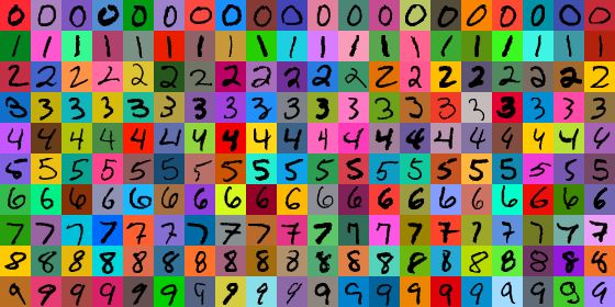
mostly consider discrete sensitive variables, such as gender or race. Therefore, we synthetically create
ColorMNIST dataset, which randomly assigns a continuous RBG color value for the background in
each handwritten digit image in the MNIST dataset (LeCun et al., 1998). We consider the background
color as sensitive information. For statistics, ColorMNIST has 60, 000 colored digit images across
10 digit labels. Similar to Section 4.1, data X and Y represent images after applying arbitrary image
augmentations. Our goal is two-fold: we want to see how well the learned representations 1) perform
on the downstream classification task and 2) ignore the effect from the sensitive variable. For the
former one, we report the top-1 accuracy as the metric; for the latter one, we report the Mean Square
Error (MSE) when trying to predict the color information. Note that the MSE score is higher the
better since we would like the learned representations to contain less color information.
Methodology. We consider the FairCCLK objective Top-1 Accuracy (↑) MSE (↑)
(equation 8) as the main method. For FairCCLK , we per-
⊗b Unconditional Contrastive Learning Methods
form the sampling process {(xi , yi , zi )}bi=1 ∼ PXY Z by
InfoNCE 84.1 ± 1.8 48.8 ± 4.5
first sampling a digit image imi along with its sensitive
information zi and then applying different image augmen- Conditional Contrastive Learning Methods
tations on imi to obtain (xi , yi ). We select the uncondi- FairInfoNCE 85.9 ± 0.4 64.9 ± 5.1
FairCCLK (ours) 86.4 ± 0.9 64.7 ± 3.9
tional contrastive learning method - the InfoNCE objec-
tive (equation 1) as our baseline. We also consider the Table 3: Classification accuracy (%) under
FairInfoNCE objective (equation 4) as a baseline, by clus- the fair contrastive learning setup, and the
tering the continuous conditioning variable Z into one of MSE (higher the better) between color in an
the following: 3, 5, 10, 15, or 20 clusters using K-means. image and color prediction by the image’s
representation. A higher MSE indicates less
Results. We show the results in Table 3. FairCCLK is color information from the original image is
consistently better than the InfoNCE, where the absolute contained in the learned representation.
accuracy improvement is 2.3% and the relative improvement of MSE (higher the better) is 32.6%
over InfoNCE. We report the result of using the Cosine kernel and provide the ablation study of
different kernel choices in the Appendix. This result suggests that the proposed FairCCLK can
8Published as a conference paper at ICLR 2022
achieve better downstream classification accuracy while ignoring more sensitive information (color
information) compared to the unconditional baseline, suggesting that our method can achieve a better
level of fairness (by excluding color bias) without sacrificing performance. Next we compare to
FairInfoNCE baseline, and we report the result using the 10-cluster partition of Z as it achieves the
best top-1 accuracy. Compared to FairInfoNCE , FairCCLK is better in downstream accuracy, while
slightly worse in MSE (a difference of 0.2). For FairInfoNCE , if the number of discretized value of Z
increases, the MSE in general grows, but the accuracy peaks at 10 clusters and then declines. This
suggests that FairInfoNCE can remove more sensitive information as the granularity of Z increases,
but may hurt the downstream task performance. Overall, the FairCCLK performs slightly better than
FairInfoNCE , and do not need clustering to discretize Z.
4.3 H ARD -N EGATIVES C ONTRASTIVE L EARNING
In this subsection, we perform experiments within the hard negative contrastive learning frame-
work (Robinson et al., 2020), which considers the embedded features as the conditioning variable Z.
Different from conventional contrastive learning methods (Chen et al., 2020; He et al., 2020) that
considers learning dissimilar representations for a pair of random data, the hard negative contrastive
learning methods learn dissimilar representations for a pair of random data when they have similar
embedded features (i.e., similar outcomes from the conditioning variable).
Datasets and Metrics. We consider two visual datasets in this set of experiments. Data X and
Y represent images after applying arbitrary image augmentations. 1) CIFAR10 (Krizhevsky et al.,
2009): It contains 60, 000 images spanning 10 classes, e.g. automobile, plane, or dog. 2) ImageNet-
100 (Russakovsky et al., 2015): It is the same dataset that we used in Section 2. We report the top-1
accuracy as the metric for the downstream classification task.
Methodology. We consider the HardNegCCLK objective (equation 9) as the main method. For
⊗b
HardNegCCLK , we perform the sampling process {(xi , yi , zi )}bi=1 ∼ PXY Z by first sampling an
image imi , then applying different image augmentations on imi to obtain (xi , yi ), and last defining
zi = gθX (xi ). We select two baseline methods. The first one is the unconditional contrastive learning
method: the InfoNCE objective (Oord et al., 2018; Chen et al., 2020) (equation 1). The second one is
the conditional contrastive learning baseline: the HardNegInfoNCE , objective (Robinson et al., 2020),
and we report its result directly using the released code from the author (Robinson et al., 2020).
Results. From Table 4, first, HardNegCCLK consis-
tently shows better performances over the InfoNCE base- CIFAR-10 ImageNet-100
line, with absolute improvements of 1.8% and 3.1% on Unconditional Contrastive Learning Methods
CIFAR-10 and ImageNet-100 respectively. This sug- InfoNCE 89.9 ± 0.2 77.8 ± 0.4
gests that the hard negative sampling effectively im- Conditional Contrastive Learning Methods
proves the downstream performance, which is in accor-
HardNeg 91.4 ± 0.2 79.2 ± 0.5
dance with the observation by Robinson et al. (2020). HardNeg InfoNCE 91.7 ± 0.1 81.2 ± 0.2
CCLK (ours)
Next, HardNegCCLK also performs better than the
HardNegInfoNCE baseline, with absolute improvements Table 4: Classification accuracy (%) under
of 0.3% and 2.0% on CIFAR-10 and ImageNet-100 re- the hard negatives contrastive learning setup.
spectively. Both methods construct hard negatives by assigning a higher weight to a random paired
data that are close in the embedding space and a lower weight to a random paired data that are far
in the embedding space. The implementation by Robinson et al. (2020) uses Euclidean distances to
measure the similarity and HardNegCCLK uses the smoothed kernel similarity (i.e., (KZ + λI)−1 KZ
in Proposition 2.2) to measure the similarity. Empirically our approach performs better.
5 C ONCLUSION
In this paper, we present CCL-K, the Conditional Contrastive Learning objectives with Kernel ex-
pressions. CCL-K avoids the need to perform explicit conditional sampling in conditional contrastive
learning frameworks, alleviating the insufficient data problem of the conditioning variable. CCL-K
uses the Kernel Conditional Embedding Operator, which first defines the kernel similarities between
the conditioning variable’s values and then samples data that have similar values of the conditioning
variable. CCL-K is can directly work with continuous conditioning variables, while prior work
requires binning or clustering to ensure sufficient data for each bin or cluster. Empirically, CCL-K
also outperforms conditional contrastive baselines tailored for weakly-supervised contrastive learning,
fair contrastive learning, and hard negatives contrastive learning. An interesting future direction is to
add more flexibility to CCL-K, by relaxing the kernel similarity to arbitrary similarity measurements.
9Published as a conference paper at ICLR 2022
6 E THICS S TATEMENT
Because our method can improve removing sensitive information in contrastive learning representa-
tions, our contribution can have a positive impact on fairness and privacy, where biases or user-specific
information should be excluded from the representation. However, the conditioning variable must be
predefined, so our method cannot directly remove any biases that are implicit and are not captured by
a variable in the dataset.
7 R EPRODUCIBILITY S TATEMENT
We provide an anonymous source code link for reproducing our result in the supplementary material
and include complete files which can reproduce the data processing steps for each dataset we use in
the supplementary material.
ACKNOWLEDGEMENTS
The authors would like to thank the anonymous reviewers for helpful comments and suggestions. This
work is partially supported by the National Science Foundation IIS1763562, IARPA D17PC00340,
ONR Grant N000141812861, Facebook PhD Fellowship, BMW, National Science Foundation awards
1722822 and 1750439, and National Institutes of Health awards R01MH125740, R01MH096951
and U01MH116925. KZ would like to acknowledge the support by the National Institutes of Health
(NIH) under Contract R01HL159805, by the NSF-Convergence Accelerator Track-D award 2134901,
and by the United States Air Force under Contract No. FA8650-17-C7715. HZ would like to thank
support from a Facebook research award. Any opinions, findings, conclusions, or recommendations
expressed in this material are those of the author(s) and do not necessarily reflect the views of the
sponsors, and no official endorsement should be inferred.
R EFERENCES
Martin Arjovsky, Soumith Chintala, and Léon Bottou. Wasserstein generative adversarial networks.
In International conference on machine learning, pages 214–223. PMLR, 2017.
Sanjeev Arora, Hrishikesh Khandeparkar, Mikhail Khodak, Orestis Plevrakis, and Nikunj Saun-
shi. A theoretical analysis of contrastive unsupervised representation learning. arXiv preprint
arXiv:1902.09229, 2019.
Philip Bachman, R Devon Hjelm, and William Buchwalter. Learning representations by maximizing
mutual information across views. arXiv preprint arXiv:1906.00910, 2019.
Alexei Baevski, Henry Zhou, Abdelrahman Mohamed, and Michael Auli. wav2vec 2.0: A framework
for self-supervised learning of speech representations. arXiv preprint arXiv:2006.11477, 2020.
Gilles Blanchard, Aniket Anand Deshmukh, Urun Dogan, Gyemin Lee, and Clayton Scott. Domain
generalization by marginal transfer learning. arXiv preprint arXiv:1711.07910, 2017.
Emmanuel J Candes, Justin K Romberg, and Terence Tao. Stable signal recovery from incomplete
and inaccurate measurements. Communications on Pure and Applied Mathematics: A Journal
Issued by the Courant Institute of Mathematical Sciences, 59(8):1207–1223, 2006.
Ting Chen, Simon Kornblith, Mohammad Norouzi, and Geoffrey Hinton. A simple framework for
contrastive learning of visual representations. In International conference on machine learning,
pages 1597–1607. PMLR, 2020.
Don Coppersmith and Shmuel Winograd. Matrix multiplication via arithmetic progressions. In
Proceedings of the nineteenth annual ACM symposium on Theory of computing, pages 1–6, 1987.
Kenji Fukumizu, Arthur Gretton, Xiaohai Sun, and Bernhard Schölkopf. Kernel measures of
conditional dependence. In NIPS, volume 20, pages 489–496, 2007.
10Published as a conference paper at ICLR 2022
Ian Goodfellow, Jean Pouget-Abadie, Mehdi Mirza, Bing Xu, David Warde-Farley, Sherjil Ozair,
Aaron Courville, and Yoshua Bengio. Generative adversarial nets. Advances in neural information
processing systems, 27, 2014.
Michael Gutmann and Aapo Hyvärinen. Noise-contrastive estimation: A new estimation principle
for unnormalized statistical models. In Proceedings of the thirteenth international conference on
artificial intelligence and statistics, pages 297–304. JMLR Workshop and Conference Proceedings,
2010.
Kaiming He, Xiangyu Zhang, Shaoqing Ren, and Jian Sun. Deep residual learning for image
recognition. In Proceedings of the IEEE conference on computer vision and pattern recognition,
pages 770–778, 2016.
Kaiming He, Haoqi Fan, Yuxin Wu, Saining Xie, and Ross Girshick. Momentum contrast for
unsupervised visual representation learning. In Proceedings of the IEEE/CVF Conference on
Computer Vision and Pattern Recognition, pages 9729–9738, 2020.
R Devon Hjelm, Alex Fedorov, Samuel Lavoie-Marchildon, Karan Grewal, Phil Bachman, Adam
Trischler, and Yoshua Bengio. Learning deep representations by mutual information estimation
and maximization. arXiv preprint arXiv:1808.06670, 2018.
Yannis Kalantidis, Mert Bulent Sariyildiz, Noe Pion, Philippe Weinzaepfel, and Diane Larlus. Hard
negative mixing for contrastive learning. arXiv preprint arXiv:2010.01028, 2020.
Prannay Khosla, Piotr Teterwak, Chen Wang, Aaron Sarna, Yonglong Tian, Phillip Isola, Aaron
Maschinot, Ce Liu, and Dilip Krishnan. Supervised contrastive learning. arXiv preprint
arXiv:2004.11362, 2020.
Lingpeng Kong, Cyprien de Masson d’Autume, Wang Ling, Lei Yu, Zihang Dai, and Dani Yogatama.
A mutual information maximization perspective of language representation learning. arXiv preprint
arXiv:1910.08350, 2019.
Alex Krizhevsky, Geoffrey Hinton, et al. Learning multiple layers of features from tiny images. 2009.
Yann LeCun, Léon Bottou, Yoshua Bengio, and Patrick Haffner. Gradient-based learning applied to
document recognition. Proceedings of the IEEE, 86(11):2278–2324, 1998.
Jason D Lee, Qi Lei, Nikunj Saunshi, and Jiacheng Zhuo. Predicting what you already know helps:
Provable self-supervised learning. arXiv preprint arXiv:2008.01064, 2020.
Dong C Liu and Jorge Nocedal. On the limited memory bfgs method for large scale optimization.
Mathematical programming, 45(1):503–528, 1989.
Arnab Mondal, Arnab Bhattacharjee, Sudipto Mukherjee, Himanshu Asnani, Sreeram Kannan, and
AP Prathosh. C-mi-gan: Estimation of conditional mutual information using minmax formulation.
In Conference on Uncertainty in Artificial Intelligence, pages 849–858. PMLR, 2020.
Aaron van den Oord, Yazhe Li, and Oriol Vinyals. Representation learning with contrastive predictive
coding. arXiv preprint arXiv:1807.03748, 2018.
Taesung Park, Jun-Yan Zhu, Oliver Wang, Jingwan Lu, Eli Shechtman, Alexei A Efros, and Richard
Zhang. Swapping autoencoder for deep image manipulation. arXiv preprint arXiv:2007.00653,
2020.
Alec Radford, Jong Wook Kim, Chris Hallacy, Aditya Ramesh, Gabriel Goh, Sandhini Agarwal,
Girish Sastry, Amanda Askell, Pamela Mishkin, Jack Clark, et al. Learning transferable visual
models from natural language supervision. arXiv preprint arXiv:2103.00020, 2021.
Joshua Robinson, Ching-Yao Chuang, Suvrit Sra, and Stefanie Jegelka. Contrastive learning with
hard negative samples. arXiv preprint arXiv:2010.04592, 2020.
Olga Russakovsky, Jia Deng, Hao Su, Jonathan Krause, Sanjeev Satheesh, Sean Ma, Zhiheng Huang,
Andrej Karpathy, Aditya Khosla, Michael Bernstein, et al. Imagenet large scale visual recognition
challenge. International journal of computer vision, 115(3):211–252, 2015.
11Published as a conference paper at ICLR 2022
Bernhard Schölkopf, Alexander J Smola, Francis Bach, et al. Learning with kernels: support vector
machines, regularization, optimization, and beyond. MIT press, 2002.
Abhishek Sinha, Jiaming Song, Chenlin Meng, and Stefano Ermon. D2c: Diffusion-denoising models
for few-shot conditional generation. arXiv preprint arXiv:2106.06819, 2021.
Le Song, Kenji Fukumizu, and Arthur Gretton. Kernel embeddings of conditional distributions: A
unified kernel framework for nonparametric inference in graphical models. IEEE Signal Processing
Magazine, 30(4):98–111, 2013.
Jean-Francois Ton, CHAN Lucian, Yee Whye Teh, and Dino Sejdinovic. Noise contrastive meta-
learning for conditional density estimation using kernel mean embeddings. In International
Conference on Artificial Intelligence and Statistics, pages 1099–1107. PMLR, 2021.
Yao-Hung Hubert Tsai, Tianqin Li, Weixin Liu, Peiyuan Liao, Ruslan Salakhutdinov, and Louis-
Philippe Morency. Integrating auxiliary information in self-supervised learning. arXiv preprint
arXiv:2106.02869, 2021a.
Yao-Hung Hubert Tsai, Martin Q Ma, Muqiao Yang, Han Zhao, Louis-Philippe Morency, and Ruslan
Salakhutdinov. Self-supervised representation learning with relative predictive coding. arXiv
preprint arXiv:2103.11275, 2021b.
Yao-Hung Hubert Tsai, Martin Q Ma, Han Zhao, Kun Zhang, Louis-Philippe Morency, and Ruslan
Salakhutdinov. Conditional contrastive learning: Removing undesirable information in self-
supervised representations. arXiv preprint arXiv:2106.02866, 2021c.
Yao-Hung Hubert Tsai, Yue Wu, Ruslan Salakhutdinov, and Louis-Philippe Morency. Self-supervised
learning from a multi-view perspective. In ICLR, 2021d.
Michael Tschannen, Josip Djolonga, Paul K Rubenstein, Sylvain Gelly, and Mario Lucic. On mutual
information maximization for representation learning. arXiv preprint arXiv:1907.13625, 2019.
Catherine Wah, Steve Branson, Peter Welinder, Pietro Perona, and Serge Belongie. The caltech-ucsd
birds-200-2011 dataset. 2011.
Mike Wu, Milan Mosse, Chengxu Zhuang, Daniel Yamins, and Noah Goodman. Conditional negative
sampling for contrastive learning of visual representations. arXiv preprint arXiv:2010.02037,
2020.
Yang You, Igor Gitman, and Boris Ginsburg. Large batch training of convolutional networks. arXiv
preprint arXiv:1708.03888, 2017.
Aron Yu and Kristen Grauman. Fine-grained visual comparisons with local learning. In Proceedings
of the IEEE Conference on Computer Vision and Pattern Recognition, pages 192–199, 2014.
12Published as a conference paper at ICLR 2022
A C ODE
We include our code in a Github link: https://github.com/Crazy-Jack/
CCLK-release
B A BLATION OF D IFFERENT C HOICES OF K ERNELS
We report the kernel choice ablation study for FairCCLK and HardNegCCLK (Table 5). For the
FairCCLK , we consider the synthetically created ColorMNIST dataset, where the background color
for each image digit image is randomly assigned. We report the accuracy of the downstream
classification task, as well as the Mean Square Error (MSE) between the assigned background color
and a color predicted by the learned representation. A higher MSE score is better because we
would like the learned representations to contain less color information. In Table 5, we consider the
following kernel functions: RBF, Polynomial (degree of 3), Laplacian and Cosine. The performances
using different kernels are consistent.
For the HardNegCCLK , we consider the CIFAR-10 dataset for the ablation study and use the top-1
accuracy for object classification as the metric. In Table 5, we consider the following kernel functions:
Linear, RBF, and Polynomial (degree of 3), Laplacian and Cosine. The performances using different
kernels are consistent.
Lastly, we also provide the ablation of different σ 2 when using the RBF kernel. First, the performance
trend does change too much and is sensitive to different bandwidths for the RBF kernel. In Table 7
we show the result of using different σ 2 in the RBF kernel. We found that using σ 2 = 1 significantly
hurts performance (only 3.0%), using σ 2 = 1000 is also sub-optimal. The performances of σ 2 =
10, 100, 500 are close.
C A DDITIONAL R ESULTS ON CIFAR10
In Section 4.3 in the main text, we report the results of HardNegCCLK as well as baseline methods
on CIFAR10 dataset by training with 400 epochs using 256 batch size. Here we also include the
results with larger batch size (512 batch size) and longer training time (1000 epochs). The results are
summarized in Table 6. For reference, we name the training procedure with 256 batch size and 400
epochs setting 1 and the one with 512 batch size and 1000 epochs as setting 2. From Table 6 we
observe that HardNegCCLK still has better performance comparing to HardNegInfoNCE , suggesting
that our method is solid. However, the performance differences shrink between the vallina InfoNCE
method and the Hard Negative mining approaches in general because the benefit of hard negative
mining mainly lies in the training efficiency, i.e., spend less training iteration on discriminating the
negative samples that have been already pushed away.
D FAIRInfoNCE ON C OLOR MNIST
Here we include the results of performing FairInfoNCE on the ColorMNIST dataset as a baseline. We
implemented FairInfoNCE based on Tsai et al. (2021c), where the idea is to remove the information
of the conditional variable by sampling positive and negative pairs from the same outcome of the
conditional variable at each iteration. Same as our previous setup in Section 4.2, we evaluate the
results by the accuracy of the downstream classification task as well as the MSE value, both of
which are deemed higher as the better (as we want the learned representation to contain less color
information, so a larger MSE is desirable because it means the representation contains less color
information for reconstruction.) To perform FairInfoNCE and condition on the continuous color
information, we need to discretize the color variable using clustering method such as K-means. We
use K-means to cluster samples based on their color variable, and we use the following numbers of
clusters: {3, 5, 10, 15, 20}.
As shown in Table 8, with the number of clusters increasing, the downstream accuracy first increases
then drops, peaking at number of clusters being 10. The MSE values continue increase as number
of clusters increase. This suggests that FairInfoNCE can remove more sensitive information as the
granularity of Z increases, but the downstream task performance may decrease.
13You can also read