Understanding Climate Feedbacks and Sensitivity Using Observations of Earth's Energy Budget
←
→
Page content transcription
If your browser does not render page correctly, please read the page content below
Curr Clim Change Rep
DOI 10.1007/s40641-016-0047-5

    CLIMATE FEEDBACKS (M ZELINKA, SECTION EDITOR)

Understanding Climate Feedbacks and Sensitivity Using
Observations of Earth’s Energy Budget
Norman G. Loeb 1 & Wenying Su 1 & Seiji Kato 1

# The Author(s) 2016. This article is published with open access at Springerlink.com

Abstract While climate models and observations generally                   Introduction
agree that climate feedbacks collectively amplify the surface
temperature response to radiative forcing, the strength of the             Climate is determined by the amount and distribution of in-
feedback estimates varies greatly, resulting in appreciable un-            coming solar radiation absorbed by Earth. In response to en-
certainty in equilibrium climate sensitivity. Because climate              ergy imbalances, complex processes give rise to energy flows
feedbacks respond differently to different spatial variations in           within the atmosphere, hydrosphere, lithosphere, cryosphere,
temperature, short-term observational records have thus far                and biosphere occurring over a range of time-space scales. For
only provided a weak constraint for climate feedbacks operat-              an Earth system in equilibrium, these energy flows must pro-
ing under global warming. Further complicating matters is the              duce outgoing longwave radiation at the top of atmosphere
likelihood of considerable time variation in the effective glob-           (TOA) that is equal to the incoming absorbed solar radiation.
al climate feedback parameter under transient warming. There               The coupled nature of the system is such that external pertur-
is a need to continue to revisit the underlying assumptions                bations to the Earth’s energy budget impact all of the Earth
used in the traditional forcing-feedback framework, with an                subsystems to varying degrees. The defining challenge for
emphasis on how climate models and observations can best be                climate science is to understand and predict the timing and
utilized to reduce the uncertainties. Model simulations can                intensity of the changes for a range of space-time scales in
also guide observational requirements and provide insight on               response to natural phenomena and man’s activities.
how the observational record can most effectively be analyzed                 The Earth’s surface temperature is expected to rise between
in order to make progress in this critical area of climate                 1.5 and 4.5 °C in response to a doubling of atmospheric CO2
research.                                                                  concentrations [1]. Despite much effort by the climate science
                                                                           community, the large range of uncertainty has not narrowed
                                                                           appreciably over the past 30 years. A key reason is due to the
Keywords Climate feedback . Climate sensitivity . Satellite .              representation of climate feedbacks in climate models.
Earth radiation budget . Observational constraint                          Increased CO2 in the atmosphere alters the Earth’s energy
                                                                           balance by reducing how much thermal infrared radiation is
                                                                           emitted to space. Most of the excess energy into the system
This article is part of the Topical Collection on Climate Feedbacks
                                                                           initially ends up being stored in the ocean, but some also heats
                                                                           the atmosphere and land and melts snow and sea ice. To re-
* Norman G. Loeb
  norman.g.loeb@nasa.gov                                                   store a balance between absorbed solar radiation and outgoing
                                                                           longwave radiation, the Earth system must emit more infrared
     Wenying Su                                                            radiation to space. In the absence of other changes, a CO2
     wenying.su-1@nasa.gov                                                 doubling would require Earth’s temperature to eventually in-
     Seiji Kato                                                            crease ∼1.2 K [2]. However, temperature changes can also
     seiji.kato@nasa.gov                                                   alter other processes and properties of the climate system,
                                                                           which can lead to further changes in Earth’s energy balance
1
     NASA Langley Research Center, Hampton, VA, USA                        that can further modify temperature. In addition to an increase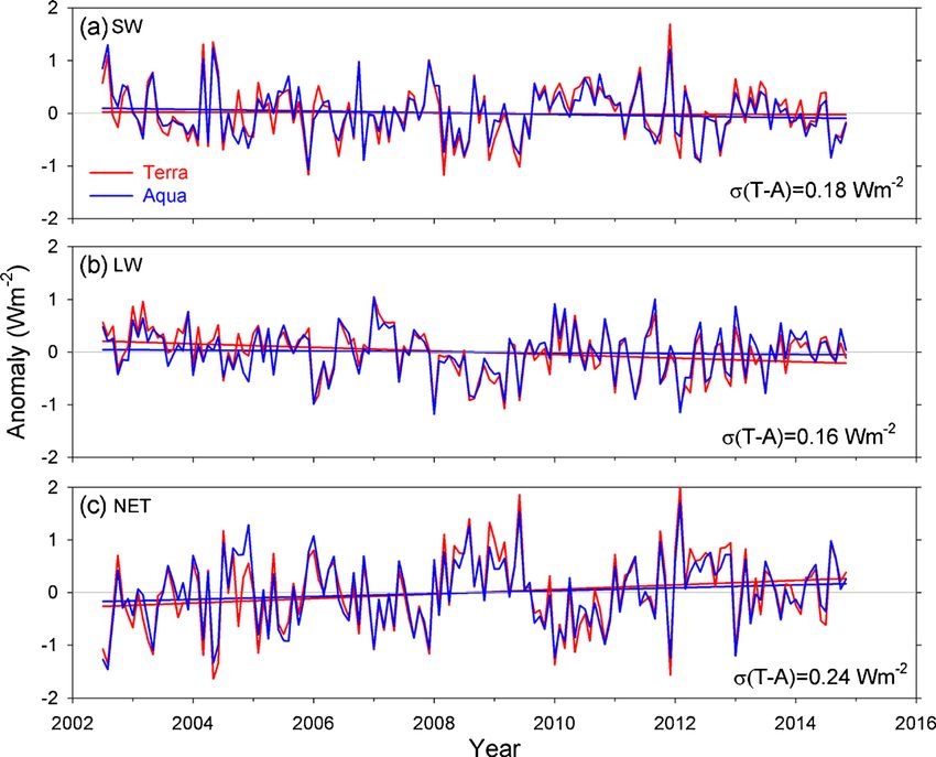
Curr Clim Change Rep

in surface temperature, feedbacks associated with water vapor,       the Earth Radiation Budget Experiment (ERBE), Forster and
clouds, snow and ice, and the vertical temperature structure of      Gregory [8] estimate via linear regression a climate feedback
the atmosphere are important. A climate feedback is quanti-          parameter of −2.3 ± 0.7 W m−2 K−1 (1σ uncertainty). Murphy
fied through its climate feedback parameter, given by the            et al. [10] used observations from both ERBE and the Clouds
change in downward TOA flux for a given temperature                  and the Earth’s Radiant Energy System (CERES) to infer a
change. Thus, an increase in downward TOA flux with                  climate feedback parameter of −1.25 ± 0.5 W m−2 K−1. More
warming temperatures yields a positive climate feedback              recently, Donohoe et al. [11] and Trenberth et al. [12] obtained
parameter.                                                           climate feedback parameters of −1.2 ± 0.5 and −1.13 ±
    Climate models agree that feedbacks collectively amplify         0.5 W m−2 K−1, respectively. By comparison, the climate
the surface temperature response to external forcing, but the        feedback parameter for a system in which only the tempera-
strength of the feedbacks varies greatly [3]. Water vapor pro-       ture or BPlanck^ feedback is operating is −3.2 W m−2 K−1.
vides the largest positive feedback, and vertical changes in         Thus, feedbacks other than the Planck feedback (e.g., water
water vapor and temperature are tightly coupled.                     vapor, clouds, snow and ice, and the vertical temperature
Accordingly, the sum of the lapse rate and water vapor feed-         structure of the atmosphere) are collectively positive and
backs are well represented by the majority of climate models.        therefore amplify the warming. An alternate approach to esti-
Feedbacks due to clouds and surface albedo (associated with          mate climate feedback and equilibrium climate sensitivity is to
snow and ice changes) are also positive in all models, but           use longer records of upper ocean heat content (OHC) change,
cloud feedbacks are the largest source of uncertainty in current     forcing, and temperature. These methods as well as others that
predictions of climate sensitivity. The main stabilizing             use satellite TOA radiation data are discussed in more detail in
(negative) feedback comes from the temperature response              Forster [13].
(Planck feedback), which is well represented in models [3].              Forster and Gregory [8] assume that changes in net TOA
    Given the large intermodel spread in climate sensitivity due     radiation due to internal variations of the system unrelated to
to uncertainties in climate feedbacks, it is reasonable to turn to   surface temperature are negligible. Spencer and Braswell
observations to help narrow the uncertainty. Recent progress         [14–16] and Lindzen and Choi [17, 18] argue that climate
on using observations to help constrain individual feedbacks         feedback determined by linear regression of short satellite
(e.g., water vapor and high clouds) is summarized in Boucher         TOA radiation and temperature records is overestimated due
et al. [4]. There is also ongoing work that relies on data from      to internal variations (e.g., natural cloud fluctuations or weath-
past climate states to estimate climate sensitivity [5]. Here, we    er noise) that can alter surface temperature directly and there-
focus on studies that use Earth Radiation Budget (ERB) sat-          by act as a source of Bnonradiative forcing.^ Clouds are typi-
ellite observations for constraining climate feedbacks operating     cally viewed as a climate feedback since in response to surface
under global warming. We briefly summarize some of the key           warming associated with a forcing, they either amplify (posi-
observational findings to date and discuss the challenges            tive cloud feedback) or offset (negative cloud feedback) the
associated with interpreting the results. We also examine the        initial forcing [19]. Based upon a simple linear box model of
state of current ERB satellite observations and explore issues       Earth, Spencer and Braswell [15, 16] claim that atmospheric
related to data analysis.                                            feedback diagnosis of the climate system remains an unsolved
                                                                     problem due primarily to the inability to distinguish between
Recent Estimates of Climate Feedbacks from Satellite                 radiative forcing and radiative feedback in satellite radiative
Measurements                                                         budget observations.
                                                                         Several studies [19–21] have pointed out significant weak-
The use of short-term satellite records to infer climate feed-       nesses in the Spencer and Braswell [14–16] and Lindzen and
back has been the subject of considerable debate. Given esti-        Choi [17, 18] analyses. Murphy and Forster [20] and Dessler
mates of radiative forcing, it is possible to use observations of    [19] repeated their analysis and showed that when a more
the covariability between surface temperature and TOA radi-          realistic ocean mixed layer depth is used, the correct standard
ation to infer empirical estimates of climate feedback.              deviation in outgoing radiation is used, the model temperature
Following Gregory et al. [6, 7], Forster and Gregory [8] use         variability is computed over the same time interval as the
a linearized version of the Earth’s global energy balance in         observations, and the difference between the linear regression
which TOA net downward radiative flux is equated with the            slope and feedback parameter is an order of magnitude smaller
difference between TOA radiative forcing and the surface             than in Spencer and Braswell [14–16]. Thus, temperature var-
temperature change multiplied by the climate feedback param-         iations at short time scales are primarily directly driven by
eter. Since the Earth is not in radiative equilibrium, the climate   ocean-atmosphere heat exchange, not from cloud fluctuations.
feedback derived under transient warming is often referred to        The ocean-atmosphere heat exchange is largely controlled by
as effective global climate feedback in order to distinguish it      El Niño–Southern Oscillation (ENSO) events, during which
from equilibrium global climate feedback [9]. Using data from        the atmosphere gains/losses energy through variations in
Curr Clim Change Rep
surface evaporation and precipitation latent heating [22]. the global radiation budget are sensitive to spatial variations in
During a La Niña event, the ocean column takes up energy, temperature, the average long-term cloud feedback differs
resulting in cooler surface temperatures, and energy is re- from that at interannual time scales [29]. This, together with
leased to the atmosphere during El Nino events, resulting in the large uncertainty in model representation of low cloud
warmer surface temperatures. Clouds respond to these ENSO- feedback [32], points to the need for further research on how
driven forcings at interannual time scales, but many cloud short-term observations can best constrain climate feedback
variations on monthly time scales are also a result of internal operating under global warming.
atmospheric variability, such as the Madden-Julian oscillation. Coupled atmosphere-ocean simulations show considerable
This Bweather noise^ complicates the linear regression ap- time variation in the effective global climate feedback param-
proach, adding uncertainty to regression slopes derived from eter under transient warming [7, 13, 31, 33–41]. This implies
TOA radiation and surface temperature. that the apparent climate sensitivity inferred from observations
These studies have also highlighted the importance of of effective global climate feedback for different periods will
using a global domain when estimating a climate feedback differ from one another even for perfect observations. Armour
parameter. Murphy [23] showed that derivation of a climate et al. [9] argue that global climate feedback is linked to the
sensitivity with a linear regression between satellite TOA ra- time evolution of regional climate feedbacks, which depends
diation and surface temperature records for a limited region upon the time variation in the geographic pattern of surface
such as the tropics (as is done in Lindzen and Choi [17]) is ill- warming resulting from the different response times of land,
posed since heat transport between regions must also be con- ocean, and sea ice. On decadal time scales, warming of the
sidered. Accordingly, Brown et al. [24] showed that large- low-latitude oceans causes strongly negative regional feed-
scale atmospheric circulation changes are the main reason back, leading to an effective climate sensitivity that is lower
why positive unforced regional surface temperature anomalies than the equilibrium climate sensitivity. The climate evolution
in the tropics and midlatitudes are associated with positive over the next few decades will thus likely depend strongly
anomalies in regional net downward TOA radiative flux, upon the geographic variations in ocean dynamics, heat up-
whereas positive global mean surface temperature anomalies take, and transport. Other studies explain the time variation in
are associated with negative anomalies in global TOA radia- effective climate feedback through a nonlinear relationship
tive flux. between global cloud radiative forcing (CRF) and global sur-
face temperature [34, 42].
Interpreting Short-Term Climate Feedback Recently, Sherwood et al. [43] reviewed additional con-
cerns relevant to constraining climate feedback with observa-
In spite of many problems with aspects of some of the earlier tions. In the traditional framework, feedbacks are associated
studies, it remains an open question whether or not short-term with processes and properties that respond to surface temper-
climate feedback (or equivalently, effective climate feedback) ature changes. The feedbacks alter Earth’s energy balance by
derived from observations provides any insight on climate enhancing or offsetting the initial forcing. Notable examples
feedback operating under global warming (equilibrium cli- of feedbacks tied to temperature are the water vapor and snow-
mate feedback). Trenberth et al. [22] question the interpreta- ice albedo feedback. However, recent modeling studies
tion of ENSO as an analogue for exploring the forced response [44–48] have pointed out that the forcing itself can lead to
of the climate system. Using 10 years of CERES TOA radia- changes that can alter Earth’s energy balance independent of
tion and surface temperature measurements, Dessler [25] and surface temperature. For example, increased CO2 concentra-
Dessler [26] applied the methodology of Soden et al. [27] and tions can alter the vertical temperature lapse rate in the middle
Shell et al. [28] to show that climate feedbacks from short-term and lower troposphere by altering longwave radiative heating
observations and global climate model control runs are gener- rates. Solar, aerosol, or greenhouse gas perturbations can lead
ally consistent, although there are notable differences in the to horizontal variations in atmospheric heating rates and
regional pattern of cloud feedback. They also note that feed- land/ocean contrasts that can alter atmospheric circulations
backs for control and forced climate model runs are only weak- and cloud patterns. These in turn can alter the TOA energy
ly correlated, implying that short satellite records likely only budget. As such, these are not Bfeedbacks^ since they do not
provide a weak constraint on climate sensitivity. More recently, involve a response to surface temperature. Changes that occur
Zhou et al. [29] used Coupled Model Intercomparison directly due to the forcing itself, without involving the global-
Project phase 5 simulations to show that cloud feedbacks in mean temperature, are referred to as Badjustments,^ and the
response to interannual and long-term surface warming are corresponding TOA radiative imbalance change is referred to
well correlated owing to a similar low cloud cover decrease as an Beffective^ radiative forcing [43]. Because adjustments
with sea surface temperature occurring at both time scales. and feedbacks can occur on similar time scales, separating the
However, because different forcings produce different pat- two effects poses a major challenge for constraining climate
terns of warming [9, 30, 31], and many factors that influence feedback using observations. The clouds will respond toCurr Clim Change Rep
ocean/land and vertical lapse rate adjustments at the same time feedback with observational records shorter than 50 years. For
as they respond to surface temperature change. This will be example, the approach used by Forster and Gregory [8] infers
true regardless of how the forcing is imposed. Clearly, the the total climate feedback parameter through a regression of
adjustments will be much stronger immediately following a monthly or annual mean TOA radiative flux and surface tem-
large instantaneous forcing, but they will also be important perature anomalies. Thus far, the method has been applied to
over the longer term for a slower continuous radiative forcing. observational records that have been too short to yield robust
Because observation-based estimates of climate sensitivity results (e.g., 15 years or less). It is therefore an open question
and climate feedback require reliable radiative forcing data as to how long a record is necessary. It is also unclear how the
[49], uncertainties in aerosol radiative forcing remain a signif- data should be averaged, whether monthly, annually, or over a
icant source of uncertainty, particularly as observational re- longer period. Forster [13] note that the use of annual averages
cords become longer. Zelinka et al. [50] show considerable produces a larger effective climate feedback parameter (smaller
model spread in effective radiative forcing by aerosols among effective climate sensitivity, ECS) compared to the use of
global climate models, and Forster [13] notes that aerosol monthly averages. Estimates based upon longer-term
forcing is the largest contributor to uncertainty in estimates (multidecadal) upper (0–700 m) OHC tendency, radiative forc-
of effective climate sensitivity from long-time scale ing, and surface temperature data also point to a larger effective
(multidecadal) observational records (e.g., in situ estimates climate feedback (smaller ECS) [13]. Given these discrepan-
of ocean heat content change). Quaas [51] highlighted the cies, there is a need for detailed studies evaluating the strengths
observational challenges involved in quantifying the contribu- and weaknesses of the different methodologies. For example, a
tion by aerosol-cloud interactions, which dominates the uncer- model analysis similar to that performed by Chung et al. [52]
tainty in climate model radiative forcing. Because aerosol ef- may help answer some basic questions. In fact, there is a need
fects can exert significant tropospheric cloud adjustments, di- for more such model simulations to help guide climate observ-
agnosing climate sensitivity from observations is challenging ing system requirements in general (these are often referred to
[52]. as climate Observing System Simulation Experiments
(OSSEs)).
Use of Climate Models to Interpret Observations Due to the large spread in climate sensitivity among
state-of-the-art global climate models, many studies
To improve our understanding of the time dependence of cli- have explored ways of constraining model estimates of
mate feedbacks and their relationship to climate sensitivity, climate sensitivity and feedback by evaluating model
both modeling and observations are essential. However, given projections according to how closely present-day ob-
the substantial internal variability in the climate system, it is served climate is captured by the models [32, 54–61].
unclear how long an observational record is needed to con- If one or more observed climate variables exhibits a
strain climate feedback. Chung et al. [52] addressed this ques- strong relationship between present-day and future cli-
tion by analyzing climate feedbacks from coupled atmosphere- mate, then in principle, the observations can be used to
ocean model simulations using a radiative kernel approach [3, identify the models most likely to provide a more accu-
27, 28]. They computed climate feedbacks from differences rate estimate of climate sensitivity. While this approach
between climate states as a function of the length of the time has been remarkably useful for climate model evaluation
average to define the climate states and the time separation and diagnosis using historical observations, it has yet to
between the climate states. Based upon their results ([52], their produce a single widely accepted set of observational
Fig. 5f), in order to reduce the upper bound of uncertainty in constraints for narrowing the range in climate sensitivity
climate sensitivity by a factor of 2 (equivalent to a 1σ uncer- [57]. A large part of the problem is that since climate
tainty in climate feedback of 0.13 W m−2 K−1), an averaging models must be relied upon to identify the variables and
length of at least 10 years would be required to define the relationships between present-day and future climate,
climate states and the climate states would need to be separated model weaknesses/deficiencies combined with observa-
by 40 years, thus requiring an observational record of at tional error add considerable uncertainty, limiting our
least 50 years. The main driver for such a long record is from ability to narrow the range in climate sensitivity.
the cloud feedback contribution, which exhibits considerably Recently, the climate community has adopted the term
more variability than other feedback contributions (e.g., lapse Bemergent constraints^ to characterize relationships be-
rate, water vapor, and surface albedo). Importantly, the Chung tween intermodel variations in a quantity describing
et al. [52] analysis does not factor in observational uncer- some aspect of observed climate and intermodal varia-
tainties, which would further increase the length of the record tions in a future climate prediction of some quantity
needed [53]. [62]. Importantly, in order to qualify as an emergent
It is unclear whether or not alternate approaches to the constraint, the relationships must be physically explain-
radiative kernel method can be used to help constrain climate able rather than a possibly fortuitous result.Curr Clim Change Rep
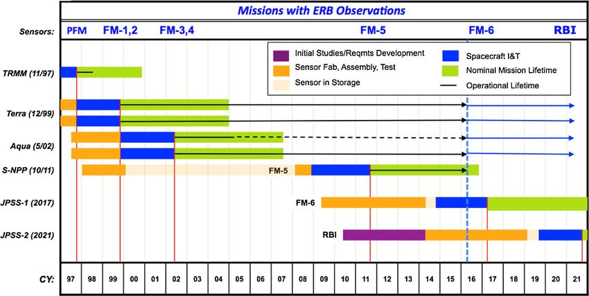
Satellite TOA ERB Data Record overlap between successive satellite missions. There is a high
probability that ERB continuity will be achieved through
Given the internal variability of the climate system, improved 2030 given the heritage and maturity of current and near-
observational constraints for climate feedback likely require future instruments and data algorithms. Figure 2 provides an
much longer (multidecadal) climate data records. Currently, estimate of the probability of a gap for the current CERES and
the longest continuous global ERB observations are from RBI flight schedule using historical spacecraft and instrument
CERES instruments flying on the Terra, Aqua, and S-NPP survival rates [65]. Although not yet official, we assume that a
satellites. A CERES instrument is scheduled for launch on second RBI instrument will fly on the JPSS-3 satellite in 2026.
JPSS-1 in 2017, and a follow-on ERB instrument called the The underlying assumption is that the mission terminates if
Radiation Budget Instrument (RBI) is being built to fly on the primary operational sensor (e.g., MODIS or VIIRS) or
JPSS-2 in 2021 (Fig. 1). spacecraft fails or if fuel becomes too low. The assumed
The reliability of satellite TOA ERB data is influenced end-of-life dates are 2025, 2021, and 2027 for Terra, Aqua,
primarily by instrument calibration uncertainty, the physical and NPP, respectively. For the case in which CERES or RBI
realism of algorithms used to infer geophysical parameters instruments fly on all available platforms (Terra, Aqua, S-
(e.g., clouds, aerosols, and radiative flux), time and space NPP, JPSS-1, JPSS-2, and JPSS-3; blue line), the probability
sampling, and the quality of the ancillary input datasets. of a gap ranges from 0.15 to 0.20 in the 2028–2030 time
Which of these factors dominate the error budget is a strong frame. The red line shows an alternate scenario, in which
function of the time-space scales that we are interested in RBI does not fly on JPSS-2 but instead flies on JPSS-3. In
resolving. At short time-space scales, the limiting factor is that case, the gap probability increases markedly to ≈0.45 in
primarily the frequency at which the observations are collect- 2028 and over 0.50 in 2030.
ed and algorithm uncertainty. At longer time-space scales, Thus far, the CERES data products have shown a remark-
radiometric stability of the instruments and long-term consis- able ability to track internal variations. To illustrate, Fig. 3a–c
tency of other input data sources matter more. Periodic shows the TOA flux anomalies from Terra and Aqua using the
reprocessing of the entire CERES record is needed to ensure latest version of CERES data products (SSF1deg-Edition4).
that the data record reflects variations in the climate system as The Terra and Aqua trends are within 0.2 Wm−2 per decade
opposed to artifacts associated with algorithm and/or input for SW and 0.3 Wm−2 per decade for LW and net at the 95 %
data changes. Combined use of CERES and imager data en- significance level. Further improvements are anticipated with
ables not only TOA fluxes but also surface radiative fluxes too the Climate Absolute Radiance and Refractivity Observatory
[63]. (CLARREO) mission, which will enable intercalibration of
Because the present generation of ERB satellite instru- many passive satellite instruments in various orbits [66]. A
ments lacks the absolute calibration accuracy needed to over- CLARREO Pathfinder mission consisting of a single reflected
come a data gap [64], it is critical that there be at least 1-year solar instrument is scheduled to fly on the International Space
Fig. 1 Flight schedule of global ERB monitoring satellite instrumentsCurr Clim Change Rep
Table 1 Effective climate feedback parameter and uncertainty (1σ) for
July 2002 to November 2014 from regression of CERES net TOA flux
and surface temperature anomalies
GISSTEMP HadCRUT4
EBAF Ed2.8 −0.89 ± 0.56 −1.12 ± 0.63
SSF1deg Ed4A (Terra) −0.74 ± 0.64 −1.10 ± 0.75
SSF1deg Ed4A (Aqua) −0.68 ± 0.61 −0.90 ± 0.69
Average −0.77 ± 0.60 −1.04 ± 0.69
Standard deviation 0.11 0.12
Fig. 2 Probability of a data gap in the global satellite ERB time series
from present through a given year. The blue curve includes all ERB
instruments flying or planned, whereas the red curve excludes the ERB (GISSTEMP) [71] and Hadley Centre Climatic Research
instrument on the J2 satellite Unit version 4 (HadCRUT4) data [72]. Given that the forcing
term for such a short period has only a small impact on the
Station in 2020 as a technology demonstration, which can in climate feedback parameter derived from this method [13], we
principal lead to a more extensive CLARREO mission as neglect that term here. The choice of CERES dataset yields an
proposed in Wielicki et al. [66]. uncertainty in the climate feedback parameter of
To estimate the uncertainty in the climate feedback param- 0.1 Wm−2 K−1 (1σ). The uncertainty due to the scatter in the
eter due to satellite TOA radiation data using the regression data is approximately 0.5 Wm−2 K−1 (1σ). Therefore, the un-
method, Table 1 shows the results using the following three certainty due to the choice of CERES dataset is a factor of 5
different CERES datasets: Energy Balanced and Filled smaller than the noise contribution to the uncertainty. The
(EBAF) Ed2.8 [67, 68], Terra SSF1deg-Month Ed4A, and choice of temperature data also matters. On average, the dif-
Aqua SSF1deg-Month Ed4A. The SSF1deg-Month Ed4A ference between climate feedback parameters inferred from
dataset was just recently released and is currently only avail- GISSTEMP and HadCRUT4 is 0.27 Wm−2 K−1. Using a
able through November 2014. It includes the latest instrument greater number of temperature datasets, Dessler and Loeb
calibration improvements [69], cloud properties, and angular [73] found that the spread in the cloud feedback parameter
distribution models [70]. We consider the common period of can be as high as 0.8 Wm−2 K−1 owing to the choice of the
July 2002 to November 2014, when all three datasets are temperature dataset.
available, and use two surface temperatures, Goddard The effective climate feedback parameter also exhibits a
Institute for Space Studies Surface Temperature Analysis surprisingly strong sensitivity to the period considered.
Fig. 3 Anomalies in global mean
TOA flux for CERES Terra and
Aqua from SSF1deg-Edition4A.
a SW, b LW, and c netCurr Clim Change Rep
Using the EBAF2.8 dataset, an effective climate feedback Table 3 Effective climate feedback parameter using monthly averages
in the regression
parameter was determined for 2001–2013 and 2001–2015
(Table 2). For the 2001–2015 period, the effective climate Data range Calibration change Effective feedback
feedback parameter decreased by a factor of 3 to 5 for monthly following gap parameter (Wm−2 K−1)
averages and 5 to 14 for annual averages compared to that for
2001–2015 None −0.35 ± 0.43
2001–2013. This is likely associated with the inclusion of the
2001–2015 (gap in 2008) None −0.19 ± 0.45
strong El Niño in 2014–2015. Consistent with Forster [13],
2001–2015 (gap in 2008) +2 % −0.25 ± 0.46
the effective climate feedback parameter tends to be larger
2001–2015 (gap in 2008) −2 % −0.14 ± 0.46
using annual averages.
In order to evaluate the influence of a data gap on satellite- Net TOA radiation data are from the CERES EBAF Ed2.8, and surface air
derived effective climate feedback parameter, we consider temperature anomalies are from GISSTEMP
monthly anomalies between 2001 and 2015 for CERES
EBAF Ed2.8 global net TOA flux and GISSTEMP surface temperature. At multidecadal time scales, coupled
air temperature (Table 3). With no data gap, the effective feed- atmosphere-ocean simulations show considerable time varia-
back parameter is −0.35 ± 0.43 Wm−2 K−1. Assuming a 1-year tion in the effective global climate feedback parameter, pro-
gap in 2008 and no calibration change following the gap, the viding a further imperative for continuing to collect stable,
e ff e c t i v e f e e d b a c k p a r a m e t e r b e c o m e s − 0 . 1 9 ± long-term climate observations. At the same time, there is a
0.45 Wm−2 K−1. However, when calibration error is intro- need to continue to revisit the underlying assumptions used in
duced by imposing a ±2 % discontinuity to the period follow- the traditional forcing-feedback framework, with an emphasis
ing the gap, the effective feedback parameter changes further on how climate models and observations can best be utilized
by ±0.05 Wm−2 K−1. Thus, in this example, introducing a gap to reduce uncertainties not only in climate sensitivity but also
of 1 year has a substantial impact on the effective feedback the spatial and temporal patterns of climate change. The cli-
parameter derivation both due to the data that is missing and to mate models can also provide important insights on the obser-
a lesser extent the calibration difference between the period vational requirements needed to make progress in this area.
prior to and after the gap. For example, dedicated climate OSSEs can help establish the
suite of climate variables that need to be observed over multi-
ple decades, at what accuracy, temporal/spatial resolution,
etc., and can also help guide how the data should most effec-
Conclusions tively be analyzed. The climate OSSE framework is also crit-
ical to help guide process-based observational requirements
The large spread in equilibrium climate sensitivity (1.5– (both satellite and field campaigns) in model development
4.5 °C) has not narrowed appreciably during the past 30 years, efforts. Ultimately, improved representation of climate feed-
owing primarily to uncertainties in the representation of cli- backs in models requires realistic, physically based parameter-
mate feedbacks in climate models. While observationally based izations. Process observations play a critical role in model
estimates suggest that climate feedbacks collectively enhance development, while longer-term observations are needed to
the temperature response to a forcing, the magnitudes of the assess model representation of climate variability and change
climate feedback parameter estimates vary greatly. Use of ob- at interannual and decadal time scales.
servations to constrain climate models and narrow the range in On the observational side, it is more critical than ever to
climate sensitivity has thus been largely unsuccessful so far. commit to sustained long-term and stable measurements of
Even with perfect observations, there are limitations to what key variables used to estimate climate feedbacks. These include
can be achieved with short observational records because differ- solar irradiance, TOA Earth radiation budget, in situ ocean
ent forcings produce different patterns of warming, and heat storage, aerosols, clouds, ice sheet and sea ice volume,
feedbacks respond differently to different spatial variations in and temperature/humidity profiles. For passive remote sensing
satellite measurements, overlap between successive missions is
Table 2 Effective climate feedback parameter for 2001–2013 and needed to avoid data gaps in the record and to ensure a
2001–2015 using monthly and annual averages in the regression
consistent calibration throughout. There is also a need to fly
Date range Monthly averages Annual averages dedicated radiance calibration missions (e.g., CLARREO)
that can help improve the accuracy and stability of a wide
GISSTEMP HadCRUT4 GISSTEMP HadCRUT4 range of passive sensors (including weather satellite instru-
2001–2013 −1.13 ± 0.52 −1.18 ± 0.58 −3.6 ± 1.6 −4.5 ± 1.8
ments) in various orbits, thereby making our observing system
2001–2015 −0.35 ± 0.43 −0.27 ± 0.47 −0.48 ± 1.1 −0.32 ± 1.1
more accurate. This represents a paradigm shift from the typical
satellite mission that targets observations of specific geo-
TOA radiation data were from the CERES EBAF Ed2.8 physical variables. However, given that the climate systemCurr Clim Change Rep
changes and feedback we are trying to observe are small com- 7. Gregory JM. A new method for diagnosing radiative forcing and
climate sensitivity. Geophys Res Lett. 2004;31:L03205.
pared to the internal variability of the climate system, and
doi:10.1029/2003GL018747.
given that at long time scales instrument calibration is the 8. Forster PM, Gregory JM. The climate sensitivity and its compo-
dominant error source, such a paradigm shift is critically nents diagnosed from Earth radiation budget data. J Clim. 2006;19:
needed. 39–52.
9. Armour KC, Bitz C, Roe GH. Time-varying climate sensitivity
from regional feedbacks. J Clim. 2013;26:4518–34.
Acknowledgments Funding for this work was provided by NASA’s 10. Murphy DM, Solomon S, Portmann RW, Rosenlof KH, Forster
Radiation Budget Measurement project. The authors would like to thank PM, Wong T. An observationally based energy balance for the
Drs. Bruce Wielicki and Bjorn Stevens for their helpful discussions and Earth since 1950. J Geophys Res. 2009;114:D17107. doi:10.1029
their leadership in this area of research. The CERES datasets were ob- /2009JD012105.
tained from http://ceres.larc.nasa.gov/compare_products.php. GISTEMP 11. Donohoe A, Armour KC, Pendergrass AG, Battisti DS. Shortwave
data were accessed on 2016-06-08 from http://data.giss.nasa. and longwave radiative contributions to global warming under in-
gov/gistemp/. HadCRUT4 were accessed on 2016-06-08 from creasing CO2. Proc Natl Acad Sci U S A. 2014;111(47):16700–5.
http://www.metoffice.gov.uk/hadobs/hadcrut4/index.html. 12. Trenberth KE, Zhang Y, Fasullo JT, Taguchi S. Climate variability
and relationships between top-of-atmosphere radiation and temper-
atures on Earth. J Geophysical Res. 2015;120(9):3642–59.
13. Forster PM. Inference of climate sensitivity from analysis of Earth’s
Compliance with Ethical Standards
energy budget. Annu Rev Earth Planet Sci. 2016;44:85–106.
14. Spencer R, Braswell BH. Potential biases in feedback diagnosis
Conflict of Interest On behalf of all authors, the corresponding author from observational data: a simple model demonstration. J Clim.
states that there is no conflict of interests. 2008;21:5624–8.
15. Spence J, Braswell BH. On the diagnosis of radiative feedback in
the presence of unknown radiative forcing. J Geophys Res.
Open Access This article is distributed under the terms of the Creative
2010;115:D16109. doi:10.1029/2009JD013371.
Commons Attribution 4.0 International License (http://
16. Spencer RW, Braswell WD. On the misdiagnosis of surface tem-
creativecommons.org/licenses/by/4.0/), which permits unrestricted use,
perature feedbacks from variations in Earth’s radiant energy bal-
distribution, and reproduction in any medium, provided you give appro-
ance. Remote Sens. 2011;3(8):1603–13.
priate credit to the original author(s) and the source, provide a link to the
Creative Commons license, and indicate if changes were made. 17. Lindzen RS, Choi Y-S. On the determination of climate feedbacks
from ERBE data. Geophys Res Lett. 2009;36.
18. Lindzen RS, Choi Y-S. On the observational determination of cli-
mate sensitivity and its implications. Asia-Pacific J Atmos Sci.
2011;47(4):377–90.
19. Dessler AE. Cloud variations and the Earth’s energy budget.
References Geophysical Res Lett. 2011;38(19):n/a-n/a.
20. Murphy DM, Forster PM. On the accuracy of deriving climate
1. IPCC. Summary for Policymakers. In: Stocker TF, Qin D, Plattner feedback parameters from correlations between surface temperature
G-K, Tignor M, Allen SK, Boschung J, Nauels A, Xia Y, Bex V, and outgoing radiation. J Clim. 2010;23(18):4983–8.
Midgley PM, editors. Climate change 2013: the physical science 21. Trenberth KE, Fasullo JT, Abraham JP. Issues in establishing cli-
basis. Contribution of working group I to the fifth assessment report mate sensitivity in recent studies. Remote Sens. 2011;3:2051–6.
of the intergovernmental panel on climate change. Cambridge: 22. Trenberth KE, Fasullo JT, O’Dell C, Wong T. Relationships be-
Cambridge University; 2013. p. 3–32. tween tropical sea surface temperature and top-of-atmosphere radi-
2. Colman R. A comparison of climate feedbacks in general circula- ation. Geophys Res Lett. 2010;37:L03702. doi:10.1029/2009
tion models. Clim Dyn. 2003;20:865–73. GL042314.
3. Soden B, Held IM. An assessment of climate feedbacks in coupled 23. Murphy DM. Constraining climate sensitivity with linear fits to
ocean–atmosphere models. J Clim. 2006;19:3354–60. outgoing radiation. Geophys Res Lett. 2010;37:L09704.
4. Boucher O, Randall D, Artaxo P, Bretherton C, Feingold G, Forster doi:10.1029/2010GL042911.
P, et al. Clouds and aerosols. In: Stocker TF, Qin D, Plattner G-K, 24. Brown PT, Li W, Jiang JH, Su H. Unforced surface air temperature
Tignor M, Allen SK, Boschung J, Nauels A, Xia Y, Bex V, Midgley variability and its contrasting relationship with the anomalous TOA
PM, editors. Climate change 2013: the physical science basis. energy flux at local and global spatial scales. J Clim. 2016;29:925–
Contribution of working group I to the fifth assessment report of 40.
the intergovernmental panel on climate change. Cambridge: 25. Dessler AE. A determination of the cloud feedback from climate
Cambridge University; 2013. p. 571–657. variations over the past decade. Science. 2010;330:1523–7.
5. Masson-Delmotte V, Schulz M, Abe-Ouchi A, Beer J, Ganopolski 26. Dessler AE. Observations of climate feedbacks over 2000–10 and
A, González Rouco JF, et al. Information from Paleoclimate comparisons to climate models*. J Clim. 2013;26(1):333–42.
Archives. In: Stocker TF, Qin D, Plattner G-K, Tignor M, Allen 27. Soden BJ, Held IM, Colman R, Shell KM, Kiehl JT, Shields CA.
SK, Boschung J, Nauels A, Xia Y, Bex V, Midgley PM, editors. Quantifying climate feedbacks using radiative kernels. J Clim.
Climate change 2013: the physical science basis. Contribution of 2008;21(14):3504–20.
working group I to the fifth assessment report of the intergovern- 28. Shell KM, Kiehl JT, Shields CA. Using the radiative kernel tech-
mental panel on climate change. Cambridge: Cambridge nique to calculate climate feedbacks in NCAR’s Community
University; 2013. p. 383–464. Atmospheric Model. J Clim. 2008;21(10):2269–82.
6. Gregory JM, Stouffer RJ, RAPER SCB, STOTT PA, RAYNER 29. Zhou C, Zelinka MD, Dessler AE, Klein SA. The relationship be-
NA. An observationally based estimate of the climate sensitivity. tween inter-annual and long-term cloud feedbacks. Geophys Res
J Clim. 2002;15(22):3117–21. Lett. 2015;42.Curr Clim Change Rep
30. Hansen J. Efficacy of climate forcings. J Geophys Res. 2005;110: 54. Allen MR, Ingram WJ. Constraints on future changes in climate and
D18104. doi:10.1029/2005JD005776. the hydrologic cycle. Nature. 2002;419:224–32.
31. Gregory JM, Andrews T. Variation in climate sensitivity and feed- 55. Knutti R, Hegerl G. The equilibrium sensitivity of the Earth’s tem-
back parameters during the historical period. Geophys Res Lett. perature to radiation changes. Nat Geosci. 2008;1:735–43.
2016;43(8):3911–20. 56. Clement AC, Burgman R, Norris JR. Observational and model
32. Bony S, Dufresne JL. Marine boundary layer clouds at the heart of evidence for positive low-level cloud feedback. Science.
tropical cloud feedback uncertainties in climate models. Geophys 2009;325(5939):460–4.
Res Lett. 2005;32:L20806. doi:10.1029/2005GL023851. 57. Klocke D, Pincus R, Quaas J. On constraining estimates of climate
33. Murphy DM. Transient response of the Hadley Centre coupled sensitivity with present-day observations through model weighting.
ocean–atmosphere model to increasing carbon dioxide. Part I: J Clim. 2011;24(23):6092–9.
Control climate and flux adjustment. J Clim. 1995;8:36–56. 58. Fasullo JT, Trenberth KE. A less cloudy future: the role of subtrop-
34. Senior CA, Mitchell JFB. Time-dependence of climate sensitivity. ical subsidence in climate sensitivity. Science. 2012;338(6108):
Geophys Res Lett. 2000;27:2685–8. 792–4.
35. Raper SCB, Gregory JM, Stouffer RJ. The role of climate sensitiv-
59. Tett SFB, Rowlands DJ, Mineter MJ, Cartis C. Can top-of-
ity and ocean heat uptake on AOGCM transient temperature re-
atmosphere radiation measurements constrain climate predictions?
sponse. J Clim. 2002;15:124–30.
Part II: climate sensitivity. J Clim. 2013;26(23):9367–83.
36. Boer GJ, Yu B. Climate sensitivity and climate state. Clim Dyn.
2003;21:167–76. 60. Sherwood SC, Bony S, Dufresne JL. Spread in model climate sen-
37. Kiehl J, Shields CA, Hack JJ, Collins WD. The climate sensitivity sitivity traced to atmospheric convective mixing. Nature.
of the Community Climate System Model, version 3 (CCSM3). J 2014;505(7481):37–42.
Clim. 2006;19:2584–96. 61. Tan I, Storelvmo T, Zelinka MD. Observational constraints on
38. Williams KD, Ingram WJ, Gregory JM. Time variation of effective mixed-phase clouds imply higher climate sensitivity. Science.
climate sensitivity in GCMs. J Clim. 2008;21(19):5076–90. 2016;352(6282):224–7.
39. Winton M, Takahashi K, Held IM. Importance of ocean heat uptake 62. Klein SA, Hall A. Emergent constraints for cloud feedbacks. Curr
efficacy to transient climate change. J Clim. 2010;23:2333–44. Climate Change Rep. 2015;1(4):276–87.
40. Li C, von Storch J-S, Marotzke J. Deep-ocean heat uptake and 63. Kato S, Loeb NG, Rose FG, Doelling DR, Rutan DA, Caldwell TE,
equilibrium climate response. Clim Dyn. 2013;40:1071–86. et al. Surface irradiances consistent with CERES-derived top-of-
41. Andrews T, Gregory JM, Webb MJ. The dependence of radiative atmosphere shortwave and longwave irradiances. J Clim.
forcing and feedback on evolving patterns of surface temperature 2013;26(9):2719–40.
change in climate models. J Clim. 2015;28:1630–48. 64. Loeb NG, Wielicki BA, Wong T, Parker PA. Impact of data gaps on
42. Andrews T, Gregory JM, Webb MJ, Taylor KE. Forcing, feedbacks satellite broadband radiation records. J Geophys Res. 2009;114:
and climate sensitivity in CMIP5 coupled atmosphere-ocean cli- D11109. doi:10.1029/2008JD011183.
mate models. Geophysical Res Lett. 2012;39(9):n/a-n/a. 65. Castet J-F, Saleh JH. Satellite reliability: statistical data analysis and
43. Sherwood SC, Bony S, Boucher O, Bretherton C, Forster PM, modeling. J Spacecr Rocket. 2009;46(5):1065–76.
Gregory JM, et al. Adjustments in the forcing-feedback framework 66. Wielicki BA, Young DF, Mlynczak MG, Thome KJ, Leroy S,
for understanding climate change. Bull Am Meteorol Soc. Corliss J, et al. Achieving climate change absolute accuracy in
2015;96(2):217–28. orbit. Bull Am Meteorol Soc. 2013;94(10):1519–39.
44. Andrews T, Forster PM. CO2 forcing induces semi-direct effects 67. Loeb NG, Wielicki BA, Doelling DR, Smith GL, Keyes DF, Kato
with consequences for climate feedback interpretations. Geophys S, et al. Toward optimal closure of the Earth’s top-of-atmosphere
Res Lett. 2008;35:L04802. doi:10.1029/2007GL032273. radiation budget. J Clim. 2009;22(3):748–66.
45. Gregory J, Webb M. Tropospheric adjustment induces a cloud com- 68. Loeb NG, Lyman JM, Johnson GC, Allan RP, Doelling DR, Wong
ponent in CO2 forcing. J Clim. 2008;21(1):58–71. T, et al. Observed changes in top-of-the-atmosphere radiation and
46. Colman R, McAvaney BJ. On tropospheric adjustment to forcing upper-ocean heating consistent within uncertainty. Nat Geosci.
and climate feedbacks. Clim Dyn. 2008;36:1649–58. 2012;5(2):110–3.
47. Kamae Y, Watanabe M. On the robustness of tropospheric adjust-
69. Loeb N, Manalo-Smith N, Su W, Shankar M, Thomas S. CERES
ment in CMIP5 models. Geophys Res Lett. 2012;39.
top-of-atmosphere Earth radiation budget climate data record: ac-
48. Wyant MC, Bretherton CS, Blossey PN, Khairoutdinov M. Fast
counting for in-orbit changes in instrument calibration. Remote
cloud adjustment to increasing CO2 in a superparameterized climate
Sens. 2016;8(3):182.
model. J Adv Model Earth Syst. 2012;4:M05001. doi:10.1029
/2011MS000092. 70. Su W, Corbett J, Eitzen Z, Liang L. Next-generation angular distri-
49. Otto A, Otto FEL, Boucher O, Church JA, Hegerl G, Forster PM, bution models for top-of-atmosphere radiative flux calculation from
et al. Energy budget constraints on climate response. Nat Geosci. CERES instruments: methodology. Atmos Meas Tech. 2015;8(3):
2013;6:415–6. 611–32.
50. Zelinka MD, Andrews T, Forster PM, Taylor KE. Quantifying com- 71. Hansen J, Ruedy R, Sato M, Lo K. Global surface temperature
ponents of aerosol-cloud-radiation interactions in climate models. J change. Rev Geophys. 2010;48:RG4004. doi:10.1029/2010
Geophysical Res. 2014;119(12):7599–615. RG000345.
51. Quaas J. Approaches to observe anthropogenic aerosol-cloud inter- 72. Morrice CP, Kennedy JJ, Rayner NA, Jones PD. Quantifying un-
actions. Curr Clim Change Rep. 2015;1(4):297–304. certainties in global and regional temperature change using an en-
52. Chung E-S, Soden BJ, Clement AC. Diagnosing climate feedbacks semble of observational estimates: the HadCRUT4 data set. J
in coupled ocean–atmosphere models. Surv Geophys. 2012;33(3- Geophys Res. 2012;117:D08101. doi:10.1029/2011jd017187.
4):733–44. 73. Dessler AE, Loeb NG. Impact of dataset choice on calculations of
53. Leroy S, Anderson J, Dykema J, Goody R. Testing climate models the short-term cloud feedback. J Geophysical Res. 2013;118(7):
using thermal infrared spectra. J Clim. 2008;21(9):1863–75. 2821–6.You can also read