UCN Detection System for the PanEDM Experiment - reposiTUm
←
→
Page content transcription
If your browser does not render page correctly, please read the page content below
Diplomarbeit

         UCN Detection System for
          the PanEDM Experiment

    Ausgeführt zum Zwecke der Erlangung des akademischen Grades

                         Diplom-Ingenieur
            Eingereicht an der Technischen Universität Wien,
                 ausgeführt am Institut Laue Langevin
      in Zusammenarbeit mit der Technischen Universität München
                                  von
                       Magdalena Pieler
                        Matrikelnummer 1325595

                                Betreuer:
           Em. Univ. Prof. Dipl.-Ing Dr.techn. Gerald Badurek,
                  Prof. Dr.sc.nat. Peter Fierlinger und
                      Dipl.-Phys. Dr. Hanno Filter

Magdalena Pieler, Ort, Datum                         Prof. Gerald Badurek
Affidavit
The following measurements and data evaluation conducted for the following thesis
were done between September 2019 and May 2021. The measurements were mainly
done at the Institut Laue-Langevin in Grenoble. There also were two measurement
campaigns at the TRIGA reactor in Mainz. Due to the pandemic the final measure-
ments done by me were delayed from March 2020 to November 2020. The later mea-
surements were conducted by Hanno Filter.

The experimental work in Grenoble and Mainz was done in cooperation with, and
under supervision of Hanno Filter.

I, Magdalena Pieler, hereby testify that the presented work has been carried out and
written by myself. No other sources and informations, other than those mentioned,
were used. Every passage or information, which was taken from the literature has
been sufficiently labeled as such.

     Magdalena Pieler, Ort, Datum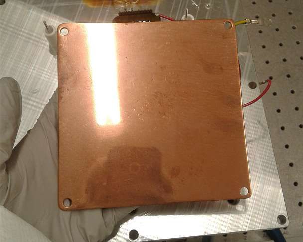
Abstract
The baryon asymmetry observed in the universe can not be explained by the cur-
rent Standard Model (SM) of particle physics [1]. An electric dipole moment of the
neutron (nEDM, dn ) could (partially) explain the abundance of matter and would be
physics beyond the SM [2]. The PanEDM collaboration prepares an nEDM measure-
ment, aiming for a sensitivity better than dn
Kurzfassung
Die bestehende Barionen Asymmetrie im heutigen Universum kann nicht durch das
Standard Modell der Teilchenphysik (SM) erklärt werden [1]. Ein elektrisches Dipol-
moment des Neutrons (nEDM, dn ) könnte (teilweise) die Asymmetrie erklären und
Physik über das SM hinaus bedeuten [2]. Die PanEDM Kollaboration bereitet ein
Experiment vor, um das nEDM mit einer Sensitvität besser als dn
Contents
1 Introduction                                                                                                         1
2 Selected Aspects of Neutron Physics                                                                                  2
  2.1   Ultra Cold Neutrons . . . . . . . . . . . . . . . . . .            .   .   .   .   .   .   .   .   .   .   .    2
  2.2   Absorption of Neutrons . . . . . . . . . . . . . . . .             .   .   .   .   .   .   .   .   .   .   .    3
  2.3   Reflection of Neutrons on an Ideal, Lossless Surface                .   .   .   .   .   .   .   .   .   .   .    3
  2.4   EDM of the Neutron . . . . . . . . . . . . . . . . . .             .   .   .   .   .   .   .   .   .   .   .    4
  2.5   Neutron Sources . . . . . . . . . . . . . . . . . . . . .          .   .   .   .   .   .   .   .   .   .   .    4
        2.5.1 Thermal Neutrons . . . . . . . . . . . . . . .               .   .   .   .   .   .   .   .   .   .   .    4
        2.5.2 UCN and VCN Production . . . . . . . . . .                   .   .   .   .   .   .   .   .   .   .   .    4

3 Ramsey Spectroscopy for nEDM Measurements                                                                             7
  3.1   The false EDM Signature of falsely classified Events . . . . . . .                              .   .   .   .    8
        3.1.1 Additional Counted Events (e. g. Background) . . . . . .                                 .   .   .   .    8
        3.1.2 Multiplicative Factor of Counted Events (e.g. Efficiency)                                 .   .   .   .   10
        3.1.3 Depolarization . . . . . . . . . . . . . . . . . . . . . . . .                           .   .   .   .   10
  3.2   The PanEDM Experiment Setup . . . . . . . . . . . . . . . . . . .                              .   .   .   .   11
  3.3   Two Chambers EDM Measurements . . . . . . . . . . . . . . . .                                  .   .   .   .   13

4 Introduction to Neutron Detection                                                                                    15
  4.1   Proportional Counters . . . . . . . . . . . . . . . . . . . . . .                      .   .   .   .   .   .   15
        4.1.1 Gas Electron Multiplier Foils . . . . . . . . . . . . . .                        .   .   .   .   .   .   16
        4.1.2 Spectrum Deformation due to a Solid Converter Film                               .   .   .   .   .   .   17
  4.2   PanEDM’s Requirements for a Detector . . . . . . . . . . . .                           .   .   .   .   .   .   19
        4.2.1 Detection Efficiency Limit . . . . . . . . . . . . . . . .                        .   .   .   .   .   .   19
        4.2.2 Background Limits . . . . . . . . . . . . . . . . . . . .                        .   .   .   .   .   .   20
        4.2.3 Expected Count Rate . . . . . . . . . . . . . . . . . . .                        .   .   .   .   .   .   21

5 Cascade Detectors                                                                                                    23
  5.1   Detector Hardware . . . . . . . . . . . . . . . .      .   .   .   .   .   .   .   .   .   .   .   .   .   .   23
  5.2   Mode of Operation . . . . . . . . . . . . . . . .      .   .   .   .   .   .   .   .   .   .   .   .   .   .   24
  5.3   Signal Processing Line . . . . . . . . . . . . . .     .   .   .   .   .   .   .   .   .   .   .   .   .   .   26
  5.4   Computer Interface and Software . . . . . . . .        .   .   .   .   .   .   .   .   .   .   .   .   .   .   27
  5.5   Gas Distribution . . . . . . . . . . . . . . . . . .   .   .   .   .   .   .   .   .   .   .   .   .   .   .   28
  5.6   Detection Efficiency . . . . . . . . . . . . . . . .    .   .   .   .   .   .   .   .   .   .   .   .   .   .   30
  5.7   Algorithm for Analyzing Pulse Height Spectra           .   .   .   .   .   .   .   .   .   .   .   .   .   .   32
6 3Helium Detector 36
6.1 Detection Efficiency . . . . . . . . . . . . . . . . . . . . . . . . . . . . . . 36
6.2 Exemplary Pulse Height Spectrum . . . . . . . . . . . . . . . . . . . . . 38
7 Improvements of the Cascade Detector 39
7.1 Measurements with the initial Cascade Make-up . . . . . . . . . . . . . 39
7.2 The Spacers between the Electrode and Detector Chassis . . . . . . . . 42
7.3 The Spacer between the Electrode and GEM Foil . . . . . . . . . . . . . 43
7.4 Variation of the Distance between Electrode and GEM foil. . . . . . . . 45
7.5 Alternatives to the CDT Electrode . . . . . . . . . . . . . . . . . . . . . 46
7.5.1 Copper Electrode . . . . . . . . . . . . . . . . . . . . . . . . . . . 46
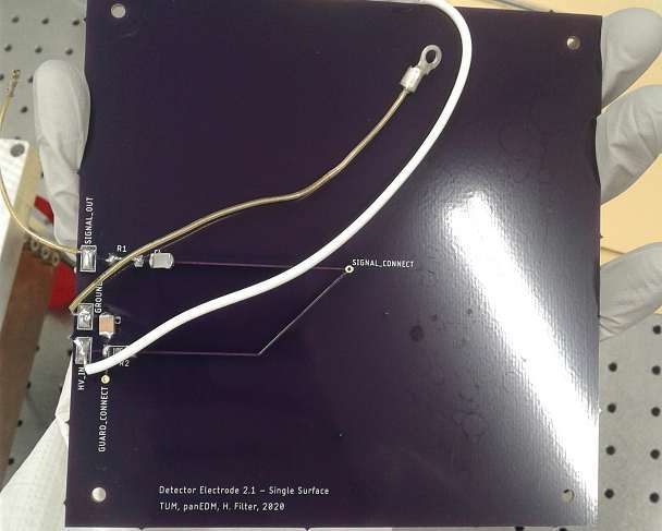
7.5.2 Circuit Board Electrode . . . . . . . . . . . . . . . . . . . . . . . 48
7.6 CDT DAQ Box Repairs . . . . . . . . . . . . . . . . . . . . . . . . . . . . 49
8 Tuning of the Cascade Detector 50
8.1 High Voltage Variation . . . . . . . . . . . . . . . . . . . . . . . . . . . . 50
8.2 Variation of the Comparator Threshold, Vref . . . . . . . . . . . . . . . . 53
8.3 Counting Gas Composition . . . . . . . . . . . . . . . . . . . . . . . . . 54
8.4 Flow of Ar/CO2 . . . . . . . . . . . . . . . . . . . . . . . . . . . . . . . . 55
9 Characterizations of the Improved Cascade Design 59
9.1 Detection Efficiency . . . . . . . . . . . . . . . . . . . . . . . . . . . . . . 59
9.2 Background . . . . . . . . . . . . . . . . . . . . . . . . . . . . . . . . . . 66
9.2.1 Neutron Background at the Measurement Site . . . . . . . . . . 66
9.2.2 Intrinsic Background of the Cascade Detectors . . . . . . . . . . 69
9.3 Detection Bandwidth . . . . . . . . . . . . . . . . . . . . . . . . . . . . . 71
10 Outlook 75
10.1 Detection Efficiency . . . . . . . . . . . . . . . . . . . . . . . . . . . . . . 75
10.2 Signal Processing Chain . . . . . . . . . . . . . . . . . . . . . . . . . . . 77
11 Conclusion 79
12 Acknowledgements i
List of Figures ii
List of Tables iv
1 Introduction
Motivation
In today’s universe we observe a large excess of matter over antimatter. This imbal-
ance is called baryon asymmetry [5]. The abundance of matter has puzzled physicists
for a long time, as the Standard Model (SM) offers no mechanism to cause it [1]. In
1966 A.D. Sakharov formulated three criteria that have to be fulfilled for there to be
baryon asymmetry [6]. One of these criteria is the violation of the CP-symmetry.
The SM allows CP-violating mechanisms [7]: the phase in the CKM matrix which
manifests itself in the observed CP-violating decay of the K, B and D-Meson ([8–10])
and the yet unobserved CP-violating therm θ̄QCD in the QCD Lagrangian which is
constrained by the electric dipole moment of the neutron (nEDM) [11], with the SM
prediction of the nEDM is dn =10−32 ecm these contributions are to small to account
for the baryon asymmetry [1, 2]. A value bigger than that could (partially) explain
the baryon asymmetry and demonstrate physics beyond the SM [2].

Thesis Outline
PanEDM is among several collaborations working to improve the current limit of the
nEDM of (0.0 ± 1.3) × 10−26 ecm [7]. The PanEDM experiment sets out to achieve a
sensitivity of dn =7.9 × 10⁻²⁸ ecm [3]. Like other nEDM experiments, PanEDM uses
stored ultra cold neutrons (UCN) to perform a Ramsey spectroscopy with separated
oscillating fields [3]. As high precession measurements require a high precision de-
tection system with low systematic uncertainties the focus of this thesis is to define
criteria whether a detection system is "good enough" for PanEDM. Furthermore, the
hardware of an existing detection system consisting of four detectors CASCADE - U
1 D -100 detectors [4], was significantly improved. Optimal operating parameters are
searched for, and subsequently the improved set up is tested for suitability for the
PanEDM measurement.

                                         1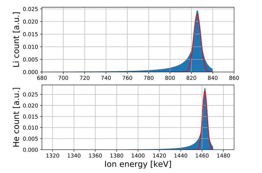
2 Selected Aspects of Neutron
  Physics
The neutron, discovered in 1932 by Chadwick as the neutral part of the nucleus
[12]. The neutron today is thought of as a composite particle of two up quarks
and a down quark. The current limit of its electrical charge is compatible with zero
((−0.2 ± 0.8) × 10−21 e) [13]. A free neutron has a half life of (879 ± 6) s [14]. As
neutrons have to be released from the nucleus their production in large quantities
is coupled to big research facilities. Two main production mechanisms are used, a
nuclear reactor (e.g. Institut Laue-Langevin, ILL) or a spalliation source (e.g. Paul
Scherrer Institut, PSI). Neutrons are characterized by their energy, respectively their
temperature or wavelength. For most experiments the neutrons from fission (~1 MeV
[15]) are too fast and have to be thermalized (~25 meV [15]) or cooled. At the lower
end of the neutron energy spectrum are the very cold (~100 µeV [16]) and ultra cold
neutrons (~100 neV [17]).

2.1 Ultra Cold Neutrons
A neutron which is totally reflected under any angle of incident is called ultra cold
neutron or UCN [17], a definition which is not always practicable. A neutron can have
an energy low enough to be reflected under all incident angles by copper (less than
168 neV [17]) but not by aluminum (less than 54 neV [17]). Frequently neutrons are
referred to as UCN if their energy is low enough so that they can be stored for some
time in some materials. UCN are of interest because they can be stored, guided and
manipulated. This allows to study fundamental properties of the neutron but also
fundamental physics in general, e.g. neutron half life [18], the nEDM [7] or the inter-
action of UCN with the gravitational potential [19].
In a solid, neutrons are exposed to the periodic potential of the strong interaction. If
the neutron is very slow, a few m s−1 , its wavelength becomes big (for 5 m s−1 = 4 nm)
compared to the distance between each delta-function-like shaped strong interaction
potentials of nuclei. These potentials can therefore be averaged, the resulting poten-
tial is called Fermi Potential, EF [17]:

                                         2πh̄2
                                    EF =       Na.                                 (2.1)
                                          m
It is dependent on the number density, N, and the positive scattering length, a, of
the respective solid. The transition from vacuum into a solid can be described as

                                           2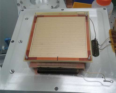
a potential step with height EF . In the classical description every neutron with a
kinetic energy perpendicular to the surface, E⊥ , smaller than the potential step will
be reflected.

2.2 Absorption of Neutrons
When a neutron beam interacts with matter the absorbed fraction, A, of the neutrons
can be calculated by the Beer-Lambert law:
                                          A = 1 − edNσT ,                                          (2.2)
d refers to the distance travelled through the material, N to the number density and
σT to the total cross section relevant to the process at the respective wavelength. If,
for example, the transmitted fraction is of interest σT is the σabs the absorption cross
section plus σscatt the scattering cross section. If the fraction absorbed due to a nuclear
process is of relevance σT is σabs . For neutrons slower than thermal neutrons σabs is
proportional to v1 1 , values in reference books are generally given for a velocity of
2200 m s−1 . If the neutrons have a different velocity the value has to be corrected, by
multiplying with the ratio of 2200 over v, the velocity of the neutron. For very slow
neutrons, like UCN and VCN, the perturbation due to the Fermi Potential (see Eq. (2.1))
                                                                                           1 mv2
can not be neglected. The velocity, has to be corrected becoming v =                      2m 2     − EF
[17] , where m is the mass of the neutron.

2.3 Reflection of Neutrons on an Ideal, Lossless
    Surface
If the surface is infinitely large and the absorption probability of the neutron when
the wave function penetrates the solid is neglected, the solid’s surface can be de-
scribed by a potential step of the height of the Fermi potential EF , see Eq. (2.1). The
Schrödinger equation can be solved and the amplitude of the reflected wave is the
reflected fraction of neutrons, | R|2 :
                                            √      √
                           2   ( k − k )2  ( E⊥ − E⊥ − EF )2
                       | R| =             = √      √           ,                    (2.3)
                               ( k + k )2  ( E⊥ + E⊥ − EF )2
with | R|2 being the reflected part of the wave, k and k are the wavenumber of the
incident and the reflected wave and E⊥ is the energy of the neutron perpendicular to
the surface [17]. Neutrons with an energy perpendicular to the surface smaller than
the potential step EF will be totally reflected. The reflection of UCN on a real surface
depends on factors such as the roughness of the surface, but their influence is hard to
formalize. Therefore the ideal approximation will be used in further considerations.
 1 Forhigher energies there are resonances in the absorption cross section resulting in great deviations
   from this rule of thumb.

                                                   3
2.4 EDM of the Neutron
As a composite particle of 3 charged quarks the neutron has an electrical dipole
moment (nEDM) [20]. The Standard Model (SM) prediction of the nEDM is around
dn =10−32 ecm [2]. The nEDM violates the CP-Symmetry but its value predicted by
the SM is to small to account for the observed baryon asymmetry. A value above the
predicted value would not only be physics beyond the SM but also could (partially)
explain the observed baryon asymmetry in today’s universe. The strongest limit for
the nEDM was published in 2020: the nEDM is smaller than (0.0 ± 1.3) × 10−26 ecm [7].
There are collaborations around the world working on improving the current limit
like n2EDM at the Paul Scherrer Institut in Switzerland, nEDM at TRIUMF in Canada
and the PanEDM experiment, a collaboration between the Institute Laue Langevin
and the TU München.
2.5 Neutron Sources
The following section is an overview of neutron sources that were employed in the
scope of this master thesis and their properties.
2.5.1 Thermal Neutrons
241
AmBe Source
241
AmBe source is often used as a laboratory neutron source because it is, compared to
other neutron sources, easily available. The neutron production occurs in two steps,
first the radioactive decay of 241Am resulting in a neptunium and an alpha particle,
see Eq. (2.4), followed by an alpha-particle-induced decay of the beryllium resulting
in a carbon atom and the desired neutron [21]:
241 237
Am → Np + 4α
9
(2.4)
Be + 4α → 12
C + n.
The resulting neutrons have an energy of a few MeV, the source is therefore often
surrounded by polyethylene, PE. The neutrons scatter on the PE’s hydrogen atoms
and are thermalized. The result is a very steady but low neutron output, with a high
gamma background.
2.5.2 UCN and VCN Production
PF2
At the beam position PF2 at the Institut Laue-Langevin (ILL) a vertical and curved
neutron guide extracts neutrons directly from a "cold source", a bath of liquid D2
at 25 K, next to the reactor core [22]. This region has a flux of thermal neutrons of
4Figure 2.1: Schematic overview of the D2 cold source and turbine at PF2,
ILL. The graphic is taken from [22].
4.5 × 1014 cm−2 s−1 [22]. The neutrons are extracted vertically so they lose energy
due to their climb against the gravitational potential, see Fig. 2.1. The beam is then di-
vided, half of it is used at the VCN beam. According to the ILL the VCN beam is, to this
day, the highest flux VCN source in the world [23]. The maximum velocity at the VCN
beam, when a neutron super mirror2 is used, is around 80 m s−1 [24]. The other half is
further slowed down by the so called Steyerl turbine. Inside the turbine a wheel turns
with about half of the velocity of the neutrons.
In repeating collisions with the blades of the turbine neutrons are further slowed
down and become UCN [22].
There are four UCN ports with slightly different spectra and densities because of dif-
ferent extraction geometries. The total UCN flux is 2.6 × 104 cm−2 s−1 , still being the
UCN source with the highest flux in the world [23]. A publication from 2017 compar-
ing UCN sources with a standard storage vessel puts the density at (4.30 ± 1.97) cm−3
after 50 s of storage time [25].
SUN2
SUN2 is a super-thermal neutron source. These are sources which can produce a UCN
spectrum colder than the temperature of the moderator [26]. SUN2’s moderator is
superfluid 4He below 1 K, in which neutrons with a wavelength of 0.89 nm lose part of
2A sequence of thin films which reflect neutrons up to a certain velocity.
5their energy by exciting a phonon in the 4He [27]. The low temperature prevents up-
scattering events so that UCN can accumulate [3]. A publication from 2017 comparing
UCN sources using a standard storage vessel puts the density at (4.09 ± 0.01) cm−3
after 50 s of storage time [25]. The storage time constant, a time constant describing
the exponential decay of the neutron population inside the storage vessel, measured
with this standard vessel is the largest of the compared sources [25]. Storage time
constants are dependent on neutron loss factors such as neutron decay and loss on
reflection. When comparing storage time constants of the same vessel of different
UCN sources the only difference is the velocity spectrum. The longer the time constant
the slower the UCN spectrum. This means that SUN2 has the slowest UCN spectrum
of all the compared neutron sources.
TRIGA
The UCN source at the TRIGA in Mainz is a super-thermal neutron source with solid
Deuterium, sD2 , as a moderator [28]. While the conversion factor to UCN of sD2 is
about 30 times larger than that of 4He the life time of UCN in the converter is only
70 ms [28]. Since this would prevent the accumulation of UCN, the produced UCN are
extracted and accumulated in a separate volume [28]. In the standard storage vessel
a density of (1.05 ± 0.01) cm−3 after 50 s could be achieved [25].
63 Ramsey Spectroscopy for nEDM
Measurements
Figure 3.1: Ramsey spectroscopy technique. The graphic is taken from [2].
Ramsey spectroscopy, the method of using separated oscillating fields for molecu-
lar beam resonance measurements was first suggested and demonstrated in 1950 by
N. Ramsey [29]. Today it is a widely used technique, from atom clocks to neutrons
bouncing in the gravitational potential [30]. The PanEDM experiment determines the
nEDM by performing Ramsey spectroscopy on UCN stored in a chamber with a high
electric field, E. The measured quantity is the polarization of the UCN. At the start
the UCN are polarized so that one spin state is predominantly occupied. A magnetic
guide field, B0 , defines the quantization axis. After a short pulse from an additional
magnetic field, B1 (ωr ), the spins begin to precess around the axis of the guide field
for a period called the free precession time, τ, see Fig. 3.1. The frequency with which
the neutrons precess is called the Larmor frequency νL . νL ∝ |µn B0 + dn E|, µn is
the magnetic dipole moment of the neutron. After a second short magnetic pulse
the neutrons will align themselves along the guide field once more. With, among
other things, the polarity of the electric field and the form of B1 (ωr ) the polarization
changes resulting in so-called Ramsey fringes. At the center of the fringes the EDM
shifts the polarization by [2]
2dn E
δPZ = P0 τ. (3.1)
h̄
7δPZ is the deviation resulting from the electric interaction, E is the electric field, dn
is the nEDM and P0 the initial polarization. The statistical uncertainty of PZ can be
approximated as [2]
1
σPZ ≈ , (3.2)
N↑ + N↓
where N↑ and N↓ are the numbers of neutrons with spin up and spin down.
3.1 The false EDM Signature of falsely classified
Events
In this section the influence of counting errors on an nEDM measurement is estimated.
A counting error or falsely classified event is every count of the detector without
unperturbed UCN from the storage chamber as a source. This can be neutron back-
ground, events inside the region of interest1 without a neutron as a source or depolar-
ized UCN. Neutron background can come from other experiments near by or result
from cosmic radiation. Events inside the region of interest can be sparks inside the
detection volume, particles other than neutrons or injected signals. With every re-
flection in the guiding system there is a possibility for UCN to get depolarized. UCN
depolarized before the Ramsey sequence lower the initial polarization, P0 and there-
fore the sensitivity of the measurement. If a neutron changes it’s spin state after the
Ramsey sequence a false EDM signature is the result. These sources of false events
can be differentiated depending on their effect on the neutron count rate. Neutron
background and events inside the region of interest are additional counted events.
Depolarized neutrons transfer one count from N↑ to N↓ or the other way around.
Furthermore, there are be processes which lead to a number of additional or lost neu-
trons proportional to the count rate, e.g. variation in the gas flow through a detector.
All of the above have in common that the measured polarization PZ changes, result-
ing in a deviation from the real polarization, δPZ . To calculate the resulting apparent
("false") EDM signature Eq. (3.1) can be rearranged as
δPZ h̄
d˜n = . (3.3)
2EP0 τ
3.1.1 Additional Counted Events (e. g. Background)
PZ is the polarization calculated from the number of neutrons with spin up N↑ and
the number of neutrons with spin down N↓ ,
N↑ − N↓
PZ = . (3.4)
N↑ + N↓
1 All counts inside this range of channels are defined as neutrons, see Section 5.7.
8The polarization with a counting error, e.g the detector measuring N↑ counts addi-
tional events ΔN↑ is:
N↑ + ΔN↑ − N↓
PZΔN↑ = . (3.5)
N↑ + ΔN↑ + N↓
The deviation from the real polarization is PZΔN↑ -PZ :
2ΔN↑ N↓
δPZΔN↑ = . (3.6)
( N↑ + ΔN↑ + N↓ )( N↑ + N↓ )
The false EDM because of this counting error can be calculated by inserting δPZΔN↑
into Eq. (3.3):
ΔN↑ N↓ h̄
d˜n = . (3.7)
( N↑ + ΔN↑ + N↓ )( N↑ + N↓ )( EP0 τ )
Taking the specific values for PanEDM into account there would be the following
false EDM signals depending on the polarization Pz and the number of additional
counted neutrons:
Figure 3.2: Plot showing the false EDM resulting from one, two and three
falsely counted additional neutron(s) per measurement se-
quence, labeled f.c.e. (false characterized event/s), depending
on the polarization.
For all specific false EDM values in Fig. 3.2, Fig. 3.3 and Fig. 3.4 N↑ + N↓ = 19900
UCN s per measurement sequence are assumed. The values of E, P0 and τ are taken
from [3].
93.1.2 Multiplicative Factor of Counted Events (e.g. Efficiency)
By considerations similar to above, one obtains a term for the deviation from the
polarization if, e.g the detector counting N↑ is wrong by a multiplicative factor, f ,
(2N↑ N↓ )( f − 1)
δPZ f = . (3.8)
( N↑ · f + N↓ )( N↑ + N↓ )
With the deviation η = f − 1, the false EDM signature caused by η is given by:
(2N↑ N↓ )ηh̄
d˜n = . (3.9)
( N↑ · f + N↓ )( N↑ + N↓ )( EP0 τ )
This leads to a false nEDM of:
Figure 3.3: Plot showing the false EDM resulting from a η of 10−5 , 5 × 10⁻⁵
and 10−4 per measurement sequence plotted versus the polar-
ization.
3.1.3 Depolarization
The effect of depolarized neutrons on the nEDM measurement can be estimated as
follows. Depolarized UCN result e.g. in additional counted N↑ → N↑ + ΔN↑ and less
counted N↓ → N↓ − ΔN↓ , resulting in a deviation, δPZDepol , of the polarization
2(ΔN↑ N↑ + ΔN↓ N↓ )
δPZDepol = . (3.10)
( N↑ + ΔN↑ + N↓ − ΔN↓ )( N↑ + N↓ )
10The result is a false EDM of:
Figure 3.4: Plot showing the false EDM resulting from one, two and three
depolarized UCN per measurement sequence plotted versus the
polarization.
Note that unlike the additional false characterized events discussed above the false
EDM signature resulting from depolarized neutrons is not dependent on the polariza-
tion.
3.2 The PanEDM Experiment Setup
The PanEDM experiment aims to set a new limit for the nEDM of dnMagneticly shielded Room
Polarizer
Switch
37
200
Storage Chamber I
340
Storage Chamber II
SuperSUN
1130
Spin Fliper
Polarizer
140
Detector
Figure 3.5: Sketch showing the setup between the PanEDM Experiment
and SuperSUN, based on [31]. Distances are given in mm.
magnetometers, two based on mercury and a yet to be determined number based on
cesium.
Number of UCN
closing chamber opening chamber
in the chamber
τfill τemp
B1 Pulse B1 Pulse
τ time
spin
B0
E
Figure 3.6: Sketch showing the evolution of the spin and the number of
UCN inside the storage chambers during one measurement se-
quence of the PanEDM Experiment. The black lines show the
UCN population inside each chamber, for the emptying and fill-
ing phase the actual curve is being displayed. Loss during the
storage period is exaggerated to be visible in this scale. Parts of
the graphic are taken from [2].
The UCN will be guided through a polarizer2 to the two storage chambers of PanEDM,
see Fig. 3.5. The chambers will be filled with UCN for a time τ f ill , see Fig. 3.6. Inside
the chamber the magnetic guide field B0 provides the quantization axes and aligns
2 Only during SuperSUN phase I.
12the spins. Then the valves of the storage chambers are closed. A short pulse of the B1
field will flip the UCN spin by π/2 and the Larmor precession starts, see the red pulse
in Fig. 3.6. After the free precession time τ, another B1 pulse will align the spins once
again with the guide filed B0 . The emptying/filling valve will be opened, indicated
by a pink stripe in Fig. 3.6. To measure the resulting polarization of the Ramsey se-
quence, the UCN are emptied into two detectors per chamber. A polarizer in front of
each detector selects one spin state so both states can be detected simultaneously, see
Fig. 3.5. Spin flippers in front of each polarizer allow to switch the detected spin states
between detectors, a measure to better understand systematic errors. Each measure-
ment sequence will last 400 seconds, 250 s of free precession time τ, 75 s filling time,
τ f ill and 75 s of emptying time, τemp [3]. After two ILL cycles (~100 days of measure-
ment) during phase I the statistical limit is estimated to be 1 × 10⁻²⁷ ecm [3]. Because
of the lower number of UCN during the first phase of SuperSUN the final limit of
7.9 × 10⁻²⁸ ecm will not be reached until phase II.
3.3 Two Chambers EDM Measurements
The considerations in Section 3.1 are based on an nEDM measurement with one UCN
storage chamber and simultaneous spin-state detection. As described in the previous
section the PanEDM experiment will have two storage chambers with anti-parallel
electric fields. Therefore an EDM would produce a shift of polarization in opposite
directions in the two chambers. A second chamber adds complexity to the setup but
it allows "to cancel in first order fluctuations of the common magnetic field3 and of
the frequency of the oscillating field4 , intensity fluctuations of nonstatistical origin
and the common part of the pick-up from high voltage on the electrical circuits" [32].
For each detector the electric dipole moment can be calculated with [32]:
N+ − N−
dU,L
1,2 = h , (3.11)
2( E+ + E− ) ∂N
∂ν
d is the electric dipole moment, the indices refer to detector 1 or 2 of the upper (U)
and lower (L) chamber. N+ and N− are the neutron numbers with a parallel or anti-
parallel electric field in respect to the guide field, B0 . E+ and E− are the electric field
intensities and ν is the frequency of the oscillating field, B1 . ∂N
∂ν is the slope of the
Ramsey fringes at the measurement point. The nEDM measurements described in
[32–35] calculated the EDM by averaging over all detectors:
1
dn = dU U L L
1 + d2 + d1 + d2 . (3.12)
4
3 In this thesis refered to as guide field, B0 .
4 In this thesis refered to as B1 .
13In Section 3.1 the collective electric dipole moment for both detectors of one chamber
was considered. In analogy with Eq. (3.12) the EDM can be calculated with:
1 U
dn = d + dL . (3.13)
2
For Poisson and Gaussian distributed uncertainties the first order effect on the EDM
signature is:
2 2
1 U 1 L
Δdn = Δdn + Δd . (3.14)
2 2 n
The combination of the two chambers always results in a smaller uncertainty than
the evaluation of one chamber5 . The combined false EDM signature resulting from
falsely classified events can be calculated by inserting the false EDM signatures (see
Section 3.1) of both chambers into Eq. (3.13). The combined false EDM is therefore less
or equal to the larger false EDM. Thus the false EDM of a single chamber setup can be
used as an upper bound for the effect of falsely classified events on a two chamber
measurement.
5 For ΔdU L
n = Δdn , Δdn is √1 ΔdU
n
2
144 Introduction to Neutron
Detection
The current best measurement of the neutron electrical charge is compatible with zero
[13]. Therefore all usual neutron detection principals are based on conversion of neu-
trons into ions. Materials with large neutron capturing cross sections are used, which
capture a neutron and undergo a nuclear reaction that produces ion/s. Typical ma-
terials are 10B, 3He or 6Li. In this thesis two conversion materials are of importance,
namely Boron and Helium, with the following reactions [36]:
10
B + n → 4He + 7Li + 2.31 MeV + γ(0.48 MeV) (94 % probability)
10 4 7
(4.1)
B + n → He + Li + 2.79 MeV (6 % probability)
3
He + n → 3H + p + 0.764 MeV (4.2)
As the kinetic energy of the captured neutron is negligible compared to the energy of
the decay products (100 neV compared to MeV) its contribution to the overall energy
of the detected ions is well below detection limits1 . The same is true for the angular
momentum of the neutron, the two decay products are therefore emitted in opposite
directions 2 .
4.1 Proportional Counters
A proportional counter is a gas filled detector which signal is proportional to the
energy of the detected particle. When a particle enters the gas filled volume of the
detector and ionizes a gas atom the charge can be detected. If the particles’s energy
is bigger than the ionization energy of the gas, a number of neutral gas atoms can
be ionized. Resulting ions and electrons are accelerated by an electric field, and can
induce further ionizations. Depending on the strength of the electric field the gas
detector can be operated in different modes, see Fig. 4.1.
1 The pulse hight spectrum of a Cascade detector based on boron shows two main peaks, one Lithium
and one Helium. These peaks are separated by approximately 0.6 MeV and ≈ 1000 channels, the
energy resolution is therefore ≈600 eV, much bigger than the different energies of the incoming
slow neutrons measured.
2 The main decay channel in Eq. (4.1) is a two body decay, as the γ is not emitted immediately, but by
an intermediate exited state of the Li ion.
15Figure 4.1: The different regimes of a proportional counter, figure taken
from [36].
If the electric field is high enough to accelerate electrons resulting from the initial
ionization, so that they can ionize further collision partners, an avalanche of electrons
and ions will form. This is called gas amplification. If the voltage is chosen, such that
the resulting charge signal is proportional to the initial energy, the gas detector oper-
ates in the proportional region and is therefore called proportional counter. With even
higher electric fields the accumulated positive charge of the produced ions deforms
the electric field locally, here the gas amplification then ends [36]. This mode is called
quasi-proportional or limited proportional region, see Fig. 4.1. Hence a proportional
counter has to be operated with a voltage sufficiently high to allow gas amplification
but low enough to avoid this degenerate effect. The gas which is ionized is called
counting gas, most of the time it is a noble gas, commonly Ar. Most proportional
counters have additive compound(s) to function as a quench gas, often CO2 . The
quench gas catches some of the electrons and lowers the risk of sparks. The gas mix-
ture used during this thesis is Ar/CO2 . In the case of neutron detection, the detected
particles are a result of neutron capture reactions (e.g. Eq. (4.1) and Eq. (4.2)). They
either enter the detection volume, as it is the case for the solid neutron converter 10B
or are produced inside the detection volume, like with the gaseous neutron converter
3
He.
4.1.1 Gas Electron Multiplier Foils
Gas Electron Multiplier (GEM) foils are used as an additional amplification step in
a proportional counter. GEM foils are thin insulators, for example Kapton, with a
grid of holes coated with cooper. The size and number of the holes have an impact
on the performance of the GEM foil. Experiments show the optimal hole diameter is
comparable to the foil thickness [37]. Typically there are between 50 and 100 holes
16cm−2 [37]. Between the foil’s opposing surfaces a voltage difference of up to several
hundred volts is applied.
Figure 4.2: Electric field lines of a GEM foil, figure taken from [37].
Above the foil a quite uniform electric field lets the electrons drift towards the
holes. Inside the holes a strong electric field (for a voltage difference of 200 V the
field reaches 40 kV cm−1 [38]), see Fig. 4.2, accelerates the electrons and increasing
ionizations in the counting gas. Amplification by a factor of ~103 can be achieved
while the spacial resolution is maintained [37]. A stack of GEM foils can be used for
higher gain. E.g for a thermal neutron detector a stack of 10 GEM foils producing an
electron cascade triggered by one ion with an diameter of 2 to 3 mm [39]. Similar am-
plification factors in a classical gas amplification chamber would require 1500 V [36]
or more, while spacial resolution is not preserved, compared to the ≈ Δ 400 V of the
GEM foil. Compared to conventional proportional counters they have one disadvan-
tage, any spark can damage the thin insulating layer and conductively connect the
copper layers thereby ruining the foil. Hence GEM foils are very sensitive to dust and
need to be handled in a clean room or under a laminar flow box.
4.1.2 Spectrum Deformation due to a Solid Converter Film
In detectors with a solid neutron converter film the decay products loose energy while
exiting the film. Depending on the length of the decay product’s path through the
film, they loose energy until they reach the gas volume, reducing the energy de-
posited in the counting gas. The resulting feature of the pulse height spectrum is
called the low-energy tail, it is intrinsic to neutron detectors with a solid neutron con-
verter film, like 10B. The recorded Li and α peaks are therefore deformed towards
lower energies, see Fig. 4.3. The thicker the film of the solid converter, the bigger the
number of neutrons which loose a significant amount of energy, the more dominant
the low-energy tail becomes, see Fig. 4.4. When choosing the film thickness of the
17Figure 4.3: Simulated energy spectrum of α and Li ions resulting from neu-
tron capture events in a 200 nm 10B film, the SRIM simulation
was done by Joachim Meichelböck [31].
converter material one has to balance the efficiency of the detector against the sepa-
ration of signal from noise. The ideal film thickness varies for different applications,
faster neutrons require thicker films. When low systematic errors are of importance
and for detection of very or ultra cold neutrons a film thickness between 100 nm and
200 nm should be chosen.
18Figure 4.4: Calculated pulse height spectra for three different 10B film
thicknesses, the thickness is given in µm. Figure taken from
[40]. The thicker the film the more dominant the low-energy
tail becomes.
4.2 PanEDM’s Requirements for a Detector
A precision experiment, like PanEDM, has stringent requirements for a UCN detector.
As described in Subsection 3.1.1 falsely counted events can have a significant impact
on the result of the experiment. In the following section, three criteria are derived for
suitability of a detector for PanEDM.
4.2.1 Detection Efficiency Limit
As UCN are scarce, therefore measurements are often dominated by their statistical
uncertainty [7, 18]. Hence the detector’s efficiency needs to be as high as possible.
The statistical sensitivity after 100 days of continuous measurements during Super-
SUN’s phase I is aspired to be σdnFigure 4.5: Relation between the relative detection efficiency and the num-
ber of additional measurement days needed to reach the as-
pired statistical sensitivity.
As a usual cycle at the ILL is about 54 days long one can argue that 84 additional
measurement days would be a good limit for the additional measurement time, rel-
ative efficiency greater than 92.5% would be needed to achieve this. The ILL had on
average around 100 days of scheduled beam time5 per year during 2017 and 2020
[41].
4.2.2 Background Limits
Here limits for background in a suitable detector are formulated. In this context all
events classified as neutrons without an UCN as an origin are referred to as back-
ground. These counts can result from electronic noise, neutron background, other
particles or charge up events inside the detector. Section 3.1 describes the sensitivity
of the measurement method of PanEDM to falsely characterized events. Figure 3.2
shows that the effect of background is depending on polarization. For further con-
sideration the worst case scenario is assumed, the falsely classified event happen-
ing during a polarization close to one. For an assessment we have to differentiate
two types of falsely classified events. The first type, non-correlated background, e.g.
background from neutrons resulting from cosmic radiation. The resulting false EDM
4 It would still be possible to achieve the "100 days" limit in two reactor cycles.
5 scheduled ≥ delivered
20signature does not accumulate over many measurement sequences. The other type
can be called correlated background, e.g an event repeatedly coinciding with a spe-
cific measurement point. Which means it is possible to add up the error over many
measurement sequences. For both types a limit can be derived. If the event is non-
correlated background the measured deviation (δPZ ) from the polarization should be
smaller than the uncertainty of the polarization (σPZ ), see Eq. (3.6) and Eq. (3.2), this
is the case for:
σPZ < δPZΔN↑ for ΔN↑ > 70. (4.3)
Using an emptying time of 75 s (as planed for PanEDM [3]) this corresponds to a rate
of 1 cps. This consideration is also valid for (ΔN↓ ). For correlated background, so if
there is a correlation to a specific measurement point the limit drops drastically. Again
let us assume the worst case scenario, something only creates events at the same
point in the measurement. This could be e.g. the polarity change of the 2 × 10⁶ V m−1
electric field resulting in an electronic interference. Here the false EDM resulting from
the falsely classified event needs to be considered, see Fig. 3.2. For the first phase
of the experiment a limit of dnFigure 4.6: The development of the number of neutrons escaping the stor-
age vessel over time.
Figure 4.6 shows the emptying curve of one of the PanEDM storage chambers, as-
suming the highest UCN density the experiment can reach during SuperSUN’s phase
II. This is equivalent to emptying the vessel directly after storing the neutrons. For
phase I the rate can reach 4851 cps in the first quarter of a second after opening the
emptying valve. With the higher density of UCN in phase II 48 659 cps can be reached.
Hence a detector and its signal processing line used for the PanEDM experiment
needs to be able to process 5 kcps for phase I and 50 kcps for phase II.
225 Cascade Detectors
The CASCADE - U 1 D -100 or "Cascade detector" is a proportional counter with one
GEM foil1 . The detector is specified to be a highly efficient (more than 90% at 4 m s−1 )
UCN detector with a bandwidth of 40 MHz [43]. The detector can be equipped with
different electrodes with varying subdivision, allowing spacial resolution in stripe or
pixel form. The detector comes with a program with implemented digital 2D high
count rate measurements, the possibility of analog height spectra measurements and
a "Time of Flight" (TOF) measurement mode. PanEDM acquired four detectors, in
this thesis referred to as detector 1 to 4. Each detector is equipped with a 64 stripes
electrode to allow beam-profile measurements.
5.1 Detector Hardware
AlMg3
Boron Coating
Entrance Foil Detector Chassis
Ceramic Washer GEM-Foil
Teflon Spacer
Electrode
Spacer
Gas In Gas Out
Figure 5.1: Schematic overview of the inner make-up of a Cascade UCN
detector.
The gas volume is constructed out of a base, a top plate and a side frame milled
out of aluminum. The top plate has a 14 cm recess were an AlMg32 entrance foil
can be placed and sealed with an additional milled part. This alloy is chosen over
aluminum because of its comparably small Fermi potential 3 and higher stability. The
entrance foil seals the volume and is coated with 10B on the inner side, see Fig. 5.1.
This coating corresponds to the conversion layer of the cascade detector described
1 Sold by CDT a company in Heidelberg, Germany.
2 Aluminum alloy: 96% Al, 3.1% Mg, 0.4% Fe and 0.5% Mn.
3 The smaller the Fermi potential the slower a UCN can be while still passing the foil, see Section 2.1.
23in Chapter 4, and measures between 100 nm-200 nm. The gas volume is filled with
Ar/CO2 . Beneath the entrance foil there is the stack of GEM foil and electrode. A
Teflon frame keeps 200 µm distance between and isolates the electrode from the GEM
foil. The electrode captures electrons, a preamplifier amplifies the charge signal and
converts it into an voltage signal. As mentioned above, the electrode is divided into
64 stripes each corresponding to a distinct read out channel. When operated with
the digital output this would allow spacial resolution. For the analog readout all 64
channels are joined and read out together, spacial information is traded for energy
resolution. All channels are connected and one is linked to one preamplifier channel
via a resistance.
5.2 Mode of Operation
In the gas volume a high electric field is applied. The chassis and entrance foil are
kept at ground potential. A voltage divider (see Fig. 5.5) situated at the back of the
detector splits the applied high voltage into three. The lowest is applied to the GEM
foil top surface facing the entrance foil. The bottom side of the GEM foil receives a
higher voltage. The highest voltage is applied to the electrode4 , see Fig. 5.2.
Figure 5.2: Sketch showing the high voltage installation of the a Cascade
Detector.
When a neutron passes through the AlMg3 entrance foil and reaches the 10B coating
it will be absorbed with a probability, dependent on its velocity, see Fig. 5.3. The
following nuclear reaction has two possible decay channels described in Eq. (4.1),
both resulting in two decay products, namely a He and a Li ion emitted in opposite
directions, therefore one decay product will always enter the gas volume.
Inside the counting gas the decay product ionizes some of the atoms. The resulting
electrons are, due to the potential difference, accelerated towards the GEM foil, ioniz-
ing more and more atoms. At the GEM foil the electron cascade is further amplified,
see Section 4.1. Finally the resulting electron avalanche is captured by the electrode.
4 E.g for a high voltage input of 1450 V: VGEM,T =806 V, VGEM,B =1128 V and VE =1289 V
2410
AlMg3 B Gas Volume
Li
n
He
Figure 5.3: Schematic representation of a neutron capture in the entrance
foil of a Cascade detector.
From here the charge signal reaches the preamplifier and is amplified and converted
into a voltage signal.
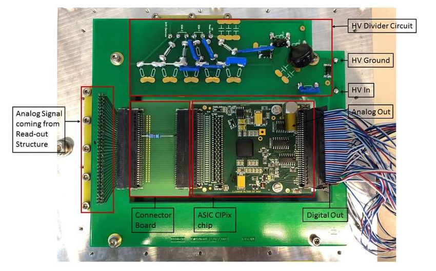
255.3 Signal Processing Line
The preamplifier of the Cascade detectors is a hybrid printed circuit AS20-3.1 board
equipped with a 64 channel ASIC CIPix 1.1 analog readout chip [44]. The AS20-3.1 is
situated at the back of the detector to minimize distance between the electrode and
the preamplifier. In this thesis these boards will be addressed as CIPix A, B, C and D.
The AS20-3.1 provides the power supply for the chip and connects it to the detector
and the analog digital converter (ADC). It has a Lemo socket were analog output can
be read out and a digital SCSI-3 connector. Measurements with an oscilloscope show
that the pulse height after preamplification is of the order of 100 mV. The DAQ-box, a
design by CDT is able to process the digital and analog output of the board, using a
Xilinx FPGA and a SU706 analog digital converter module [45]. The DAQ-box also acts
as a controller and a power supply for the CIPix. There are 10 bias voltages or currents
that can be set to control the preamplification and the digital analog conversion of the
CIPix.
Figure 5.4: Circuit diagram of the CIPix. Taken from [44].
Figure 5.4 shows the circuit diagram of the CIPix. Note that only 6 parameters
influence the analog output used during this thesis. As the AS20-3.1 board is only
designed for analog read out of one specific channel at a time, an adapter board con-
nects all the feedthroughs from the 64 channels of the electrode so that the whole
active area can be read out analogical at once. To do so the combined signal is con-
nected via a 23 Ω resistor to a preamplifier channel, this channel is than fed trough to
the Lemo socket. The resistor serves to damp spikes and prevent the CIPix channel
from burning through. Figure 5.5 shows the AS20-3.1 board with the CIPix (the black
square), the adapter board (referred to as Connector Board), the resistor connecting
the 64 channels of the electrode to the one channel of the CIPix which is fed through
to the Lemo socket (identified as Analog Out), the SCSI-3 connector (indicated as Dig-
ital Out) and the voltage divider described in Section 5.2. CDT claims that the CIPix
can handle a 330 kHz with 10% dead time [45].
26Figure 5.5: Picture of the AS20 board with the CIPix, connector board, volt-
age divider analog and digital connectors. Taken from [31].
5.4 Computer Interface and Software
DAQ Box Computer
Digtal in, low V
USB
Analog in
Hv USB,
galvanicy decoupled
HV Supply
Cascade Detector
neutrons
Gas in
Gas out
Figure 5.6: Schematic overview of the experimental setup for measure-
ments with the Cascade UCN detectors.
Figure 5.6 shows the setup for the detectors. High voltage is applied via an SHV
cable from a NIM crate module. The high voltage for each detector is individually
27addressable. The NIM module can be operated via a USB connection which is gal-
vanically decoupled. The applied voltage varies with the specific inner make-up of
the detector and ranges between 1350 V and 1450 V. The CIPix is supplied with low
voltage and controlled by the DAQ-box. They are connected via a SCSI-3 connector.
The analog signal is transmitted via a Lemo cable from the CIPix to the DAQ-box. The
DAQ -box uses an old USB .1 protocol. The USB connection can therefore not be decou-
pled from the computer by conventional solutions. The DAQ-box is therefore always
additionally grounded via the computer.
Two programs are used for the operation: a C++ program developed by CDT and
bought with the detection system. This program controls the CIPix via bias voltages
and currents set in the DAQ-box. Furthermore measurement time and ADC thresh-
old (all events in a channel smaller than the threshold are discarded as noise) can be
set. My predecessor, Joachim Meichelböck, wrote a Python program to simplify the
measurement process: it controls the high voltage, sets Vref of the CIPix (see Fig. 5.4),
the ADC threshold for the signal processing line and starts a measurement of desired
duration. It does so by writing a .txt file and executing the compiled C++ program
which then reads the file and starts a measurement with the desired settings. After
each measurement the Python program moves the files created by the C++ program
into a numbered folder and creates a file with the total number of events in each ADC
channel for each detector. This file is much smaller than the files created by the C++
program which contain the total number of events in each ADC channel for each de-
tector for time steps of about 1 s. All other parameters of the CIPix including the bias
voltages and currents and the selection which preamplifier channel can be read out
analogically can only be set by altering the C++ program.
5.5 Gas Distribution
gas bottel Ar/CO2
Gas out
Bubbler Gas in
Detector(s)
Figure 5.7: Schematic overview of the original setup for gas supply for the
Cascade UCN detectors.
The Cascade detectors need a steady flow of Ar/CO2 to prevent aging effects and
dilute contaminations of the counting gas which might occur during operation [46].
During this thesis ratios 85/15 and 90/10 of Ar/CO2 were used. When the inside of
28the Cascade has been exposed to air, it has to be flushed with Ar/CO2 for at least a few
hours before high voltage can be applied again. The first setup for the gas supply, see
Fig. 5.7, had a fine tuning valve after a pressure reducer to control the flow. The four
detectors are connected to it serially through Swagelock quick connectors. To prevent
flow of air back into the detectors, after the detectors Ar/CO2 was guided through an
isopropanol bath. Quick connectors allow to be disconnected and reconnected with
virtually no contamination of the gas atmosphere inside the system. This makes it
possible to take out a detector fix something and plug it back in with no need for
flushing the other detectors with gas. This setup provides a kind of stable flow for
the Cascade detectors. Once the fine tuning valve was set the flow slowly decreases
over days with the pressure in the gas bottle. There was no means to monitor the
absolute flow or variations of it, apart from counting bubbles in the isopropanol bath
from time to time. The setup was therefore extended to allow the gas flow to be
monitored, remotely adjusted and stabilized.
p.s. 1 p.s. 2
A A
gas bottle Ar/CO2 MFC
Gas out
p.s. 3
A
gas bottle CO2
A Gas in
MFC
p.s. 4
Detector(s)
Bubbler
Figure 5.8: Schematic overview of the gas supply setup with a mass flow
controller and pressure gauges for the Cascade UCN detectors.
A mass flow controller (MFC) EL-Flow Select from the company Bronkhorst and
pressure gauges (SPAN-PO25 from Festo) were added, see Fig. 5.8. This MFC was cal-
ibrated to Ar/CO2 with a 90/10 ratio. After the pressure gauges and the MFC a quick
connection allows to attach the detectors one after another. After the detector(s) an-
other quick connector links the detectors to another pressure gauge (SPAN-B2 from
Festo) and the gas was once again guided through isopropanol to prevent back flow
into the detectors. In the old set up a wash bottle was reconfigured to hold the iso-
propanol, in this system it was replaced by a glass bubbler. A valve was added, this
decouples, if needed, the detectors from the bubbler and makes it possible to evac-
uated and then fill the detectors with Ar/CO2 . This creates a clean gas atmosphere
inside the detector and makes flushing the detector unnecessary. A second MFC for
CO2 was foreseen and with the setting of the first MFC changed to Ar, two bottles
with clean gas could be used instead of the gas mixture. This would greatly reduce
the delivery time and the cost of the counting gas. This option is illustrated in dashed
29lines in Fig. 5.8.
5.6 Detection Efficiency
The neutron converter of a Cascade detector is a 10B coating on the inner surface of
the entrance foil of the detector. For a neutron to be detected it needs to be captured
by the boron and a resulting ion needs to reach the counting gas volume with suffi-
cient energy to ionize atoms. The probability of this is dependent on thickness of the
10
B coating, material and thickness of the entrance foil and the velocity of the neutron.
10
B coating: Contrary to prior mentions the boron coating consists not only of 10B.
There is about 5% 11B in the film. Since 10B is the main active component for the neu-
tron detection the abbreviation 10B is often used. 11B has a smaller absorption cross
section, by a factor of 105 , than 10B. Its purpose is therefore not to capture neutrons
but to lower the Fermi potential, see Eq. (2.1), reducing the reflexion of neutrons on
the film surface. In this thesis such a film will be referred to as a 10B coating/film. For
the detection efficiency of a 10B coating one has to consider the absorption probabil-
ity of the coating, see Eq. (2.2), and the probability of the ion to escape the film and
enter the gas volume were it can be detected. The escaping probability adds factors
dependent on the range of the ions in the coating to the simple Beer Lambert law [40]:
1
= {1 + σAbs (v) N ( R Max − d) − (1 + σAbs (v) NR Max )e−σAbs (v) Nd }, (5.1)
2σAbs (v) N
where σAbs (v) is the absorption cross section depending on the velocity of the neu-
tron, N is the number density, R Max is the stooping range of the ions in boron and d is
the film thickness. A derivation of this formula can be found in [40]5 . R Max is energy
dependent and therefore different for the Li, He ions and the two decay channels, see
Eq. (4.1). Taking all that into account the detection probability Det of the coating is:
Det = 0.96( He,1 + Li,1 ) + 0.06( He,2 + Li,2 ) (5.2)
Were He,1 is the efficiency for a Helium ion of the first decay channel, and so forth.
The stooping ranges of the ions were taken from [24].
Reflexion: Whenever there is a Fermi potential difference there is a probability that
neutrons are reflected, see Section 2.3. The Fermi potential is a material specific quan-
tity, see Section 2.1. For a cascade detector a neutron passes through two material
transitions and with it two Fermi potential steps. The first one is from vacuum to
AlMg3 and the second from AlMg3 to the boron coating. The first potential step has
the hight of the Fermi potential of AlMg3 (53.18 neV), the second one is the difference
between the Fermi potential of AlMg3 and the one of 10B (with 5% 11B) (54.69 neV).
5 be aware, in [40], there is a typo in the final equation, there is a R Max in the exponent of the expo-
nential and not a d.
30The reflection can be calculated with Eq. (2.3). For the reflection on the transition from
AlMg3 to 10B this equation has to be altered, to take the deceleration of the neutron
because of the Fermi potential of AlMg3 into account. The reflection on the AlMg3
foil plays a very important role for low velocities (< 10 m s−1 ). It prevents detection
of neutrons with a velocity smaller than 3.4 m s−1 , since they are totally reflected.
Absorption of the entrance foil: Additional to the reflection, the absorption in the
AlMg3 foil lowers the detection efficiency. It can be calculated with Eq. (2.2). The
scattering and absorption cross section σscatt and σabs for all elements of the alloy
need to be taken into account. For a composite the macroscopic cross section needs
to be taken into account [47].
When all these factors are considered the detection efficiency is:
10
Figure 5.9: Detection efficiency for a neutron for 3 B film thicknesses de-
pending on the neutron velocity.
The boron thicknesses depicted in Fig. 5.9 are similar to the coating thicknesses on
the entrance foils used with the Cascade detectors. The appointed thickness of the
four foils is 100 nm. As every foil is coated during its own coating process the coating
thickness may vary. An indication that this must be the case are the different colors
of the coatings.
315.7 Algorithm for Analyzing Pulse Height Spectra
Figure 5.10: Plot showing an exemplary pulse height spectrum of detector
2 at the TEST-beam.
Figure 5.10 shows an exemplary pulse height spectrum (PHS), the distribution of
counts per ADC channel, of a Cascade detector. The two high peaks are the Li and
He peak from the main decay channel, on their right side there are two small addi-
tional peaks corresponding to events from the second decay channel of 10B (around
channel 2200 and 32006 ), see Eq. (4.1). The exponential decay in the low numbered
channels is the electronic noise (around channel 500). The increase in events between
the first peak and the electronic noise is called the low-energy tail and is due to the
energy loss of ions in the boron coating, see Subsection 4.1.2 (around channel 1000).
In the channels after the peaks (3400 and upwards) there can be counts in the high
energy region resulting from sparks or charge up effects, their probability varies from
detector to detector.
To quantify the spectra an analyzing algorithm was written in Wolfram Mathematica.
This tool finds the peak positions and fits them, fits the electronic noise and estimates
its influence on the count rate, makes an estimate of the low-energy tail and suggests
a region of interest (ROI). The region of interest is the range of channels where events
will be counted as neutrons. These parameters allow the comparison of different
6 All channel specifications are not general and apply only to the PHS depicted in Fig. 5.10.
32pulse height spectra and detectors and facilitate the assessment of data as the PHS of
the different detectors vary even when they have the same inner make-up.
Peak Positions
The analysis of a PHS is performed after calculating the moving average of 4 neigh-
boring channels. To localize the two main maxima the PHS is split up into intervals.
These intervals are input values determined by looking at some PHS. The maximum
value in the interval between the noise and the second peak is picked as the approx-
imate value for the first peak, maximum peak 1. The maximum in the remaining list
is marked as the preliminary position and height of the second peak, maximum peak
2. As there can be outliers that may have the highest value but are not in the center of
the peak, the peaks are fitted for better approximation. The approximate values for
peak 1 and peak 2 are used as starting values for a nonlinear model fit, which fits a
gauss to the data in an interval around the maxima. Because of the additional peaks
(resulting from the less likely decay channel in Eq. (4.1)) and the distortion due to
the low-energy tail the peaks are not gaussian, but the deviation at the top is small.
A gauss can therefore be used to find the peak and position and fit the height. As
only around 200 data points are used to fit the peak the baseline of the peak has to
be added to the fitting model. To do so the rate in between the maxima is taken as
the baseline of the fit. The fitted maxima are then used to split the spectra in sections
were the dominating feature then can be analyzed.
Electronic Noise
The minimum before the first peak is located. As the low-energy tail becomes dom-
inant in the direction towards the first peak, the data is not exponentially decaying
until the minimum, the position is therefore divided by a factor7 . This then is the
upper limit of the data for the noise fit. The data is logarithmized, allowing then a
linear fit of the exponential decreasing. This fit is then used to calculate the electronic
noise within the region of interest, ROI.
Low-Energy Tail
The low-energy tail is a feature intrinsic to the detector. When a neutron is captured
in the boron coating its decay products looses energy while exiting the film, resulting
in an unsymmetrical peak with a distortion to the low-energy region, see Subsec-
tion 4.1.2. In absence of an analytically description a linear fit was used to describe
the tail’s first part. The data was fit from the minimum between electronic noise and
peak 1 to µ1 − f σ1 8 , with µ1 and σ1 being the expected value and the standard devi-
7 Dependent on the type of electrode used, either 3 or 2.
8 Thefactor f is, dependent on the type of electrode used, either 5 or 6. It was determined by trial and
educated guess.
33You can also read