The impact of beneficial ownership transparency on illicit purchases of U.S. property - Matthew Collin Florian M. Hollenbach David Szakonyi
←
→
Page content transcription
If your browser does not render page correctly, please read the page content below
The impact of beneficial
ownership transparency
on illicit purchases of
U.S. property

Matthew Collin
Florian M. Hollenbach
David Szakonyi

 BROOKINGS GLOBAL
 WORKING PAPER # 170
 MARCH 2022

The impact of beneficial ownership transparency
               on illicit purchases of U.S. property*

                                             Matthew Collin†
                                         & Florian M. Hollenbach‡
                                            & David Szakonyi§

                                       First Draft: August 15, 2021
                                      This Draft: February 22, 2022

                                                    Abstract
          High value real estate is a popular destination for corrupt and criminal assets, in part
      caused by limited oversight and lack of transparency in real estate transactions. In response to
      these concerns, the U.S. Treasury began implementing a series of Geographic Targeting Orders
      (GTOs) in 2016, forcing corporate buyers making all-cash purchases in targeted counties to
      report the company’s ultimate beneficial owner. To estimate the causal effect of beneficial
      ownership transparency on these types of purchases, we combine data on millions of real
      estate transactions over the period 2014-2019 with a staggered difference-in-differences design.
      Our analysis suggests the absence of an aggregate effect of the GTOs on corporate all-cash
      purchases in targeted counties, as well as little evidence of attempts to evade the program. We
      contend that the lack of overt enforcement and validation of the ownership information failed
      to create a sufficient deterrent effect to drive out participation in the sector by illicit actors.

   * Authors listed in alphabetical order. Equal authorship is implied. We thank Andrew Baker, Josh Kirschenbaumn,
Lakshmi Kumar, Jakob Miethe, Bob Rijkers, Justin Sandefur, and participants at the 2022 Empirical Research on AML
and Financial Crime Conference as well as the World Bank Symposium on Data Analytics for Anticorruption in
Public Administration. Data provided by Zillow through the Zillow Transaction and Assessment Dataset (ZTRAX).
More information on accessing the data can be found at http://www.zillow.com/ztrax. The results and opinions
are those of the author(s) and do not reflect the position of Zillow Group. Data was also generously provided by
OpenCorporates, the largest open database of companies in the world whose public benefit mission is to increase
transparency of the corporate world. More information can be found at http://www.opencorporates.com. The paper
also benefited from key support from the Anti-Corruption Data Collective (http://www.acdatacollective.org). All
remaining errors are our own.
   † World Bank, Brookings Institution Email: mcollin@worldbank.org. URL: https://sites.google.com/view/

mattcollin/home
   ‡ Associate Professor, Department of International Economics, Government and Business, Copenhagen Business

School, Porcelænshaven 24A, 2000 Frederiksberg, Denmark. Email: fho.egb@cbs.dk. URL: fhollenbach.org
   § Assistant Professor, Department of Political Science, George Washington University, Monroe 416, 2115 G St. NW,

Suite 440, Washington, DC 20052. Email: dszakonyi@email.gwu.edu. URL: http://www.davidszakonyi.com/
1     Introduction
Much of the scholarship on eradicating corruption in developing countries centers around fixing
domestic institutions and the incentive structures that enable the abuse of public office for pri-
vate gain (Olken and Pande, 2012; Ferraz and Finan, 2011). Yet a slew of recent investigations,
such as the Panama Papers, the FinCEN files, and the most recent Pandora Papers, highlight
the role that political and financial institutions in richer countries play in facilitating corrupt,
criminal, and kleptocratic activity abroad.1 The ability of bad actors to stash their illicit earn-
ings abroad incentivizes the underlying criminal activity, deprives origin countries of important
sources of revenue (Reuter, 2012; Gray et al., 2014), and produces a range of deleterious effects
in the recipient markets (Badarinza and Ramadorai, 2018; De Simone, 2015).
     Real estate markets in rich countries, in particular, are considered to be a popular target
for money laundering (FATF, 2007). Real estate assets offer many attractive features for money
launderers, including the ability to store large amounts of cash without a clear mechanism to
determine the actual market value of the asset. Moreover, in many markets real estate companies
and their agents are not covered by the same anti-money laundering (AML) provisions that
govern banks, leading to less scrutiny of the source of their clients’ wealth. While it is difficult
to determine precisely how much illicit money makes its way into foreign property markets, the
amounts observed in prosecuted money laundering cases (a significant underestimate) suggest it
is sizable. A recent study noted that $2.3 billion were laundered through U.S. real estate between
2015 and 2020 (GFI, 2021).
     Lax oversight of the real estate sector is compounded by the fact that a majority of jurisdic-
tions impose weak reporting requirements on legal entities. Rather than owning a property in
one’s name, buyers of real estate can shield their identity using shell companies - firms that do
not engage in any substantive economic activity. In recent years, shell companies have been a
key conduit for corrupt politicians from countries such as the DRC, Malaysia, and Ukraine to
buy luxury real estate in the U.S. and other advanced economies (Gabriel, 2018; White, 2020).
For example, an analysis of London properties connected to owners under investigation for cor-
    1 "ThePanama Papers: The largest investigation in journalism history exposes a shadow financial system that ben-
efits the world’s most rich and powerful.," International Consortium of Investigative Journalists, October 2020, https:
//www.icij.org/investigations/pandora-papers/. "The FinCen Files," International Consortium of Investigative
Journalists, September 2020, www.icij.org/investigations/fincen-files. "The Pandora Papers: The largest in-
vestigation in journalism history exposes a shadow financial system that benefits the world’s most rich and power-
ful." International Consortium of Investigative Journalists, October 2021, https://www.icij.org/investigations/
pandora-papers/.

                                                          1
ruption revealed that over 75% of the properties were purchased using a company based in an
offshore jurisdiction with high levels of financial secrecy (De Simone, 2015).2 In the hope of re-
ducing the ability for corrupt and criminal actors to hide behind shell companies when engaging
in economic activity, policymakers have begun introducing laws to require transparency around
“beneficial ownership,” requiring companies to disclosure who ultimately owns, benefits from,
or controls them.
    In this paper we analyze an institutional change–beneficial ownership reporting–designed to
curb illicit financial flows into high-value real estate markets in the U.S. In January 2016, FinCEN,
a bureau within the U.S. Department of Treasury tasked with combating money laundering, an-
nounced the implementation of Geographic Targeting Orders (GTOs) in two counties: Miami-
Dade and Manhattan. These orders required title insurance companies to collect information
on the beneficial owners of any legal entities purchasing real estate using only cash (‘corporate
all-cash purchases’) whenever the sales price exceeded a threshold defined at the county level.
Though the information on beneficial owners was only made available to law enforcement au-
thorities (and not the general public), the strengthened transparency was designed to increase
the probability that someone purchasing real estate with laundered money would be detected.
From 2016-2018, the GTOs were extended to an additional twenty counties, with the monetary
thresholds also being lowered to expand the breadth of property transactions covered by the
policy.
    In this study we estimate the causal effect of the GTO introduction on real estate transactions,
under the assumption that an increased probability of detection should result in a deterrence
effect, reducing the number of corporate all-cash purchases in the targeted markets. To do this,
we make use of Zillow’s Transaction and Assessment Dataset (ZTrax), which covers nearly all
residential real estate transactions in the United States over the past decade. We then exploit the
staggered roll-out of the GTO policies in certain counties and above certain price thresholds to
investigate whether the increased transparency leads market participants to adjust their behavior
following either the announcement or implementation of a GTO in a given county.
    In our main analysis, we estimate the effect of GTO policies using a staggered difference-in-
differences design. Given the multiple treatment periods and large differences in group sizes,
we use the doubly robust estimator introduced by Callaway and Sant’Anna (2021b). Across a
   2 Only 1.3% of properties in London are owned by companies based in offshore jurisdictions of this nature, sug-
gesting that the preponderance of these firms in corruption cases is not an artefact of the nature of the UK property
market.

                                                         2
number of different model specifications, we find no evidence of a sustained effect of the GTO
policy on the number, total price volume, or share of corporate all-cash purchases in targeted
counties. We also see little difference in the patterns of corporate all-cash purchases versus a
‘placebo’ outcome that should not be affected by the policy: Real estate purchases by individuals
using mortgages. In addition to the staggered difference-in-differences design, we also estimate
augmented synthetic control models as proposed by Ben-Michael, Feller, and Rothstein (2021).
Again, we find no systematic evidence that GTO policies affected the number or total value of
corporate all-cash purchases.
   We then test whether, on the margin, the GTO program led potential buyers to either target
properties just below the reporting threshold or otherwise manipulate the price so that purchases
would not be reported. When considering the distribution of purchase prices in GTO-affected
counties following the introduction of the policy, we find no evidence of bunching just below
the reporting threshold. This stands in stark contrast to bunching in purchase prices observed in
response to real estate transaction taxes in New York as reported in Kopczuk and Munroe (2015),
a finding we replicate with the ZTrax data.
   Finding no evidence of an average affect on corporate all-cash purchases, we dig in further
to test whether the GTOs had a differential effect on all-cash purchases by legal entities ’most
likely’ to be used for these illicit transactions. Merging in business registry data from OpenCor-
porates,3 we show that the GTOs did not lead to an overall decline in purchases by companies
registered by mass formation agents, all-cash purchases by companies registered in so-called
secrecy jurisdictions (Delaware, Nevada, and Wyoming), or by newly incorporated companies.
We also do not find any evidence that buyers in GTO-covered counties attempted to evade the
rules by substituting into other purchasing strategies such as using trusts (which were not cov-
ered by transparency requirement) or mortgages from foreign or bad banks. Across our different
estimations, we do find some suggestive evidence that the initial GTO in Miami and Manhattan
may have affected behavior in those real estate markets. Therefore, in the last section, we dig
deeper to investigate whether this first GTO in March 2016 produced any substantial results by
zooming in on the geographic areas ’most likely’ to have been attractive to money launderers:
Manhattan and Miami. At both the county and zip-code levels, we do not find evidence that the
GTOs differentially affected corporate all-cash purchases compared to other types of real estate
transactions not covered by the GTOs.
  3 https://opencorporates.com/

                                                3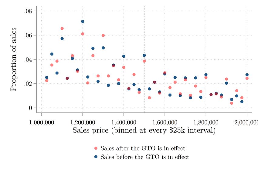
Taken together, our analysis suggests the absence of an aggregate effect of the GTOs on
corporate all-cash purchases in the targeted counties. Our findings differ sharply from those
presented by Hundtofte and Rantala (2018). Using the same underlying data but a shorter time
period, Hundtofte and Rantala (2018, 1) conclude that “all-cash purchases by corporations fall by
approximately 70%.” As we show in our paper, this finding is likely due to a misidentification
of corporate buyer types. Once corrected, there is little evidence in the data that the GTOs had
any aggregate effect on real estate market behavior.
   In the penultimate section, we discuss two possible explanations for the limited effectiveness
of the policy. The small scale explanation holds that even if the GTOs were implemented and
enforced, the amount of money laundered into high-value properties is too small to be picked up
by aggregate analysis. Although precisely defining the scale of illegal transactions prior to the
GTOs is near impossible, we argue that recent journalistic investigations as well as an internal
FinCEN evaluation demonstrate that significant amounts of suspicious money continue to flow
into GTO-covered counties. Instead, the qualitative evidence better supports an incomplete imple-
mentation explanation. Title companies may have only partially complied with the regulations,
while there has been little to no visible enforcement of the GTO orders. No properties have been
seized nor criminal investigations publicly linked to the data gathered from the GTOs. So long
as FinCEN’s capacity to ensure compliance with and visibly enforce the GTOs remains limited,
money launderers will continue to find the U.S. real estate market attractive.
   In this paper, we make several contributions to the empirical literature on anti-corruption
efforts and transparency. We are undertaking one of the first studies of an intervention specifi-
cally designed to counter illicit flows in property markets. Despite the fact that both regulators
and civil society have raised significant concerns about the abuse of this industry, few efforts
have been made to empirically evaluate the impact of policies intended to drive out illicit money
(Transparency International, 2017). In addition to Hundtofte and Rantala (2018), one of the few
studies that examines how policy can affect the laundering of wealth through property markets is
Agarwal, Chia, and Sing (2020). The authors find that in Singapore, cross-border cash limits and
enhanced real estate agent regulations lead to a reduction in the price of properties purchased
by persons linked to offshore shell companies.
   More generally, this paper contributes to a nascent literature on the impact of AML policies
on various sectors of the economy. To date, most work in this area has focused on the impact
AML regimes have had both on and through the banking sector (Slutzky, Villamizar-Villegas,

                                                 4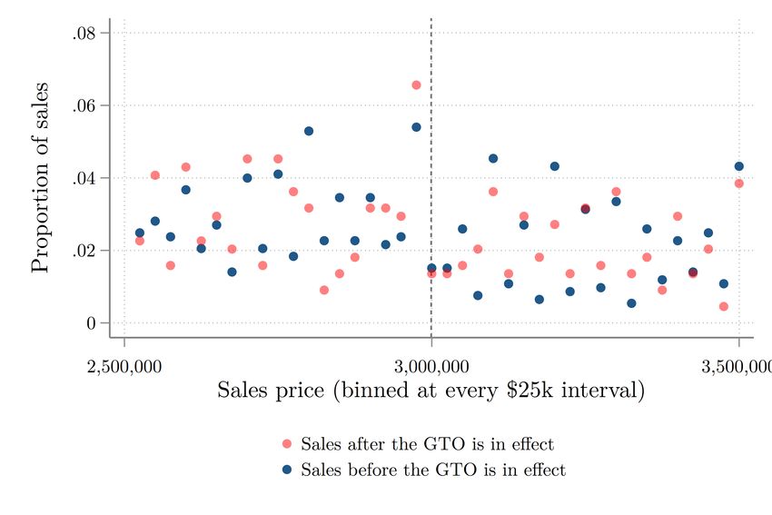
and Williams, 2020; Agca, Slutzky, and Zeume, 2021) or the aggregate impact of international
AML watch-lists (Morse, 2019).
      Our work also adds to a growing literature on how policies aimed at revealing ultimate
beneficial ownership can drive illicit wealth out of markets. This includes research on the large,
negative impact that tax transparency initiatives have on various forms of offshore wealth (Casi,
Spengel, and Stage, 2020; Menkhoff and Miethe, 2019; Beer, Coelho, and Leduc, 2019; O’Reilly,
Ramirez, and Stemmer, 2019) and a number of studies showing that removing the presumption
of anonymity can force those who previously evaded detection to come clean (Bethmann and
Kvasnicka, 2016; Londoño-Vélez and Ávila-Mahecha, 2021).
      Finally, we build upon an existing literature that examines the drivers and impacts of foreign
demand for property. For example, Badarinza and Ramadorai (2018) find that fluctuations in
economic and political risk abroad leads to changes in real estate prices in London and New
York. Similarly, Gorback and Keys (2020) find that the introduction of foreign-buyer taxes by
other countries induced an increase in Chinese housing investment in the U.S. and a subsequent
increase in housing prices. Other studies have found that foreign buyers typically buy at a
premium and are drivers of faster house price growth (Sá, 2016; Cvijanović and Spaenjers, 2020).

2     Context
2.1     Motivation

The U.S. is considered by many to be a popular destination for illicit finance. In an analysis
of grand corruption cases comprising $56 billion, a World Bank study found that corporations
and bank accounts were more likely to be established in the U.S. than any other jurisdiction
(de Willebois et al., 2011). This is partly driven by the attractiveness of investing in the U.S.
economy (Forbes, 2010), but also the perception that despite the U.S.’s role in enforcing AML
standards around the world, its own banks and corporate service providers’ compliance with
those standards is lacking (Findley, Nielson, and Sharman, 2014).
      Up until 2021, setting up a U.S.-based shell company was relatively simple, allowing individ-
uals to easily conduct business with a significant degree of anonymity. Registering a company
in the U.S. is not only inexpensive and quick, but there have been no requirements that the ben-
eficial, or true, owners of the corporation be reported to authorities at the time of registration. In
some states, this corporate registration process requires less information from an individual than
what is needed to obtain a library card (Global Financial Integrity, 2019). People from around the

                                                  5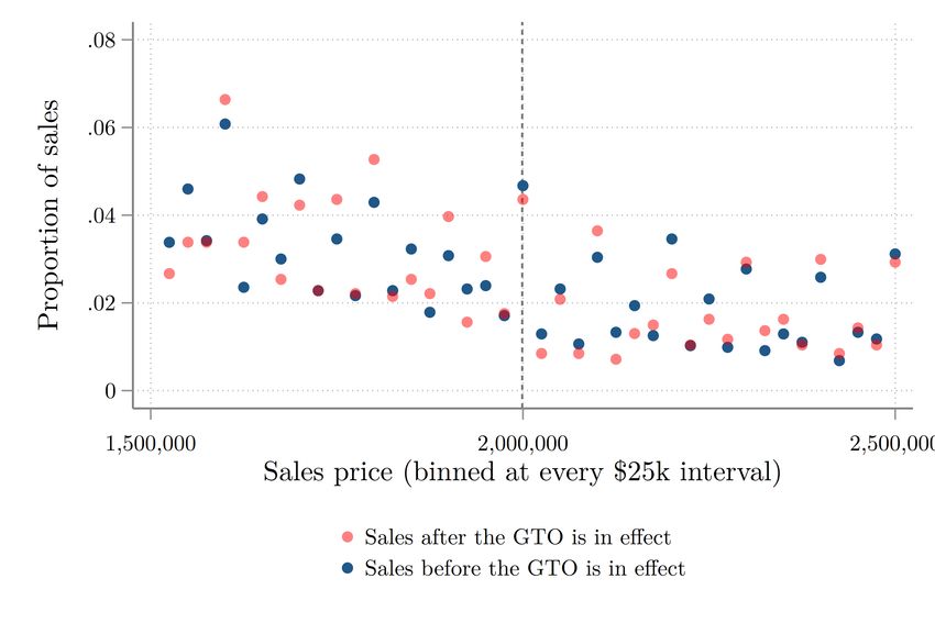
world can hire a corporation service provider to set up a U.S.-based shell company and then use
nominee officers, directors, and stockholders to shield the names of true beneficiaries from pub-
lic record (Network, 2006).4 Law enforcement officials often complain about their investigations
going cold when shell companies appear in the money trail.5
    Real estate markets appear to be an attractive target for money launders, especially in the
U.S., given the corporate secrecy conferred. Data on the predominance of real estate in money
laundering cases is somewhat scarce, but according to a survey of legal professionals around
the world by the Financial Action Task Force (FATF), an international standard-setter for AML
policies, real estate makes up approximately 30% of criminal assets confiscated in around 20
countries (FATF, 2013a). Investigative journalists have highlighted a large number of potentially-
corrupt individuals investing in U.S. property, ranging from the CEO of Equatorial Guinea’s
state-owned oil company to the individuals behind the Malaysian 1MDB scandal (Martini, 2017;
Massoko, Orphanides, and Jones, 2021). Other criminal organizations such as drug cartels, the
Italian mafia, and groups propagating Ponzi schemes have been caught moving money into U.S.
real estate using anonymous shell companies (GW, 2020; Wieder, Dasgupta, and Wang, 2021).
    The attractiveness of real estate markets to illicit finance is in part due to factors inherent
to the sector. The purchase of a high value property provides a ‘one and done’ method of
laundering a large amount of money, either to store it in a steadily appreciating asset or to resell
again, thus generating proceeds which are subsequently viewed as clean. This is compounded
by the fact that in countries such as the U.S., many of the non-financial parties involved in the
real estate market, such as brokers and lawyers, are not subject to AML regulation and are thus
not required to give the buyers nor the sellers of property much in the way of scrutiny (FATF,
2007; Martini, 2017).
    Although real estate professionals are not required by law to conduct due diligence on their
clients, financial institutions are. Consequently, illicit property purchases are more likely to be
spotted if they involve banks or similar institutions. Under the Bank Secrecy Act (BSA), financial
institutions must monitor their transactions and report any suspicious activity to FinCEN in the
form of Suspicious Activity Reports (SARs), exposing buyers that rely on external financing to
   4 The passage of the Corporate Transparency Act (2021) should undo this anonymity through the creation of a

centralized database of the beneficial owners of all companies registered in the U.S. How and when this new law will
be implemented is still under deliberation at the time of writing.
   5 Barlyn, Suzanne.        “Special Report:      How Delaware kept America safe for corporate secrecy“.
Reuters, August 24, 2016.          https://www.reuters.com/article/us-usa-delaware-bullock-specialreport/
special-report-how-delaware-kept-america-safe-for-corporate-secrecy-idUSKCN10Z1OH

                                                         6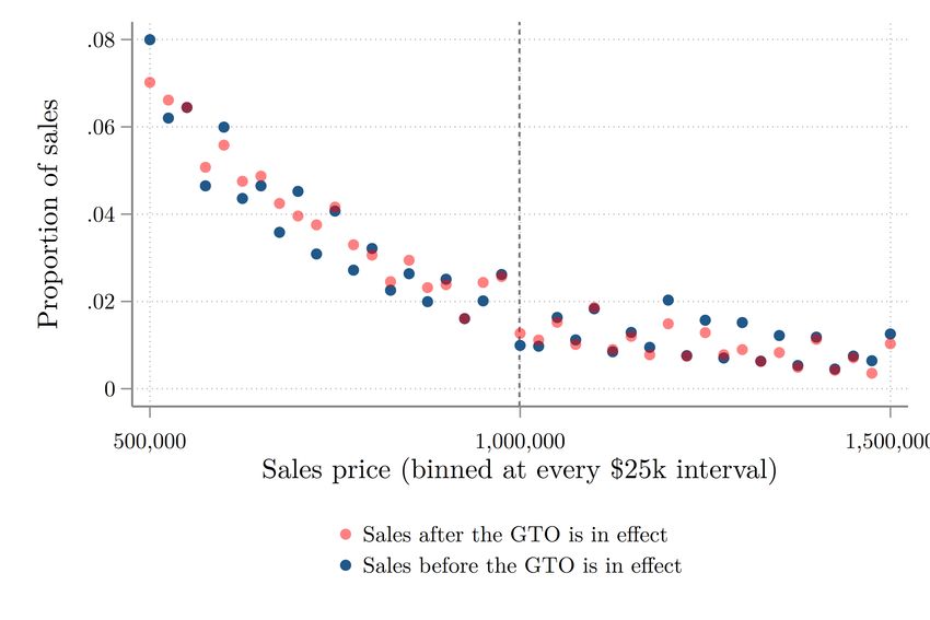
Figure 1: Cash purchases by companies become more common in the luxury property market

Notes: Figure shows local polynomial estimate of the probability a purchase is both (i) made by a corporation and
(ii) is made without a mortgage, for residential purchases over $50k and below $250m. Estimates made over every
single purchase captured by the ZTrax database between 2010 and 2015 for the for 21 counties ultimately targeted by
the GTO program (approximately 8 million observations). 95% confidence intervals shown.

more scrutiny. Since 2012, FinCEN has applied these requirements not only to ordinary banks
but also to non-bank mortgage companies and brokers. Thus, even for purchases made using
anonymous shell companies, because of due diligence requirements, any lender must still gather
information on the beneficial owner(s) of the shell company.
    Prior to the GTO program, the use of a shell company could still grant the buyer a reasonable
degree of anonymity if the purchase was made ‘in cash,’ as none of the parties in the transaction
would be subject to FinCEN’s reporting requirements. This loophole led to concerns that cor-
porate all-cash purchases have become an attractive means of investing in U.S. property while
maintaining anonymity. While it is impossible to know the share of corporate cash purchases
that are illicit, the practice is particularly prevalent with regards to luxury properties. A recent
investigation by the New York Times found that almost half of the properties priced at $5 million
and above were bought using shell companies (Story, 2015). Our own estimates using Zillow’s
data confirms a similar pattern: As illustrated in Figure 1, corporate all-cash buyers seem to
dominate both the very low and and the very high end of the property market, with around 40%
of all purchases over $100 million in GTO countries involving these types of buyers.

                                                        7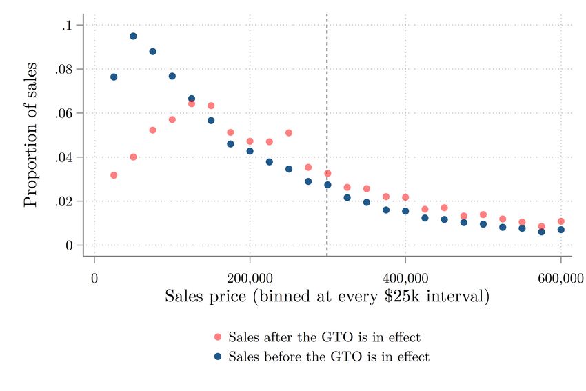
2.2     The Geographic Targeting Order program

As a response to concerns that corporate cash transactions afford buyers a high degree of secrecy,
FinCEN developed its Geographic Targeting Order (GTO) program. On January 13th, 2016,
FinCEN announced its first two GTOs for Miami and Manhattan, which were set to come into
effect on March 1st of that year and last for 180 days. The order applied to all transactions in
which a legal entity purchased a residential property, without external financing, in either cash
currency or using a check. Only properties purchased above a set price ($1 million for Miami
and $3 million for Manhattan) were covered.
      Importantly, the GTOs created a reporting requirement for title insurance companies, which
applied to any title insurance company involved with a reportable transaction. The companies
were required to collect identifying information on the person representing the legal entity in the
transaction as well as information on any and all beneficial owners (those with more than 25%
control over the legal entity). FinCEN reportedly chose title insurance companies because nearly
every buyer purchases title insurance (GAO, 2020).
      The initial order was set to expire after 180 days, but after four months, FinCEN announced
a second GTO which covered a further 12 counties. To date, FinCEN has renewed its GTO
program eight times, eventually expanding the reach of the program to counties in California,
Texas, Hawaii, Nevada, Washington, Massachusetts, and Illinois. Over the first two and a half
years of the program, FinCEN applied different price thresholds for its reporting requirements,
but eventually reduced the threshold to $300,000 for all targeted counties. Figure 2 displays the
timing of when each county was introduced to the GTO program as well as the price threshold
that was applied.
      In addition to expanding the geographic and price coverage of the GTOs, FinCEN slowly
expanded the set of monetary instruments that would be covered. As mentioned above, the first
GTO covered cashier’s, certified, and traveler’s checks as well as cash currency. In August 2016,
the scope was expanded to personal and business checks, then to all wire transfers in September
2018, and finally to virtual currencies in November 2018. While FinCEN has not updated the
scope of the GTOs in any manner since November 2018, it has continued to renew the program
every six months.
      To date, FinCEN has issued eight public GTOs. However, reports from both title insurance
companies and the Miami Herald indicate that FinCEN also issued a confidential GTO directly

                                                 8
to title insurers in April 2018, to be implemented in the subsequent month, that lowered the
reporting threshold to $300,000 (Hall and Nehamas, 2018) and expanded the range of the GTO
to “five more metropolitan areas” (Bethencourt, 2018). If these reports are correct, then the terms
of FinCEN’s publicly-released GTO from November 2018 were actually introduced six months
earlier. In our analysis of the impact of the GTOs, we test whether this confidential GTO had a
separate impact from the publicly-released GTOs.
Despite only covering twenty-two counties in total,6 the GTO program targeted both a signif-
icant share of the U.S. population and its overall housing market. In 2015, the counties covered
by the program represented about 20% of the country’s population, about 27% of the national
volume of real estate sales and more than 40% of all corporate all-cash purchases. They also
represent a sizable share of potentially-illicit behavior. GTO counties were the origin of roughly
29% of all suspicious activity reports filed by banks to FinCEN in 2015. Half of the GTO counties
are also designated by FinCEN as “High Intensity Financial Crime Areas” (HIFCAs), a special
designation for areas where authorities estimate that money laundering and financial crime is
extensive. Out of the fifty-seven money laundering cases which involved the purchase of real
estate detailed in a recent report, nearly 60% involved properties in GTO counties (GFI, 2021).
While there have occasionally been calls to expand the GTO program to other counties or to
expand its scope to other types of transactions such as commercial property, beyond Hundtofte
and Rantala (2018) there has been little analysis of the impact of the program. When interviewed
by the Government Accountability Office (GAO), FinCEN reported that–as of mid 2019–37%
of transactions reported through the GTO program involved a person who was also subject to
a suspicious activity report (SAR), a report that banks file with FinCEN when they suspect a
transaction may be facilitating money laundering (GAO, 2020). However, because it is unknown
what percentage of SARs actually reflect an illicit transaction,7 this overlap may just reflect the
tendency for banks to file SARs on similar types of transactions (large cash transfers involving
corporate buyers), rather than any underlying criminality.
6 As of 2016, there were 3,007 counties in the United States.
7 Recent research suggests that banks in the U.S. may file SARs ‘defensively,’ to avoid being punished for failing to
report an illicit transaction, leading to a low signal-to-noise ratio (Unger and Van Waarden, 2009).
9Figure 2: Public revisions to the Real Estate Geographic Targeting Orders (GTO), 2016–2020
Note: Figure shows the timing of public GTO announcements (dotted vertical line) by FinCEN and their implemen-
tation (solid vertical line) for each of the twenty-two counties ultimately included in the program. Not shown is
the confidential GTO announced in April 2018 and implemented in May 2018, which ran until the next public GTO
announcement in November 2018. Sources: FinCEN GTO announcements and GAO (2020)
103 Data and empirical framework
Our primary goal in this analysis is to identify whether the introduction of the GTO program led
to a decline in the types of transactions it was targeting: Corporate all-cash purchases made at
prices at or higher than the thresholds set by FinCEN. Because the policy was publicly announced
and implemented, we would expect the initial GTOs to have created a significant deterrence
effect. Those who would have used shell companies to buy property should substitute away into
other types of behavior, for fear of detection by the authorities. Declines in economic activity
have been observed following the introduction of similar information sharing regimes, ranging
from beneficial ownership in partnership formation (GW, 2013) to offshore deposits (O’Reilly,
Ramirez, and Stemmer, 2019).
In the rest of this section, we discuss the data we use to identify these transactions in the U.S.
property market as well as the econometric approach we take to estimate the impact of the GTOs
on these types of transactions.
3.1 ZTrax residential property data
Our primary data source on real estate transactions is Zillow’s Transaction and Assessment
Dataset (ZTrax) (ZTRAX, 2021). Zillow aggregates data from public records at the county level
using a variety of different private data providers (which are indicated in the data).8 The ZTrax
data includes separately-collected information on both deed transfers (ZTrans) and property as-
sessments (ZAsmt), which are linked by unique identifiers.
To create our sample, we start with universe of all deed transfers included in the ZTrans data
for the period 2014-2019. We keep only direct sales, removing other types of deed transfers,
such as foreclosures, second mortgages, or transfers between family members. Since GTOs do
not apply to commercial properties, we then restrict our data to only include sales of residential
properties.9 This initial data set includes over 39 million real estate transactions over ten years.
8 Eachrow has an indicator for the provider that entered the data, but Zillow does not provide a dictionary to de-
cipher the actual companies. Below we describe both how using the different data providers affects the measurement
of several key variables and how we account for resulting differences.
9 For more details on the creation of our sample, see Section A.1 in the Appendix. ZTrax is primarily a dataset
of residential property transactions, preventing us from analyzing commercial properties as placebo or substitution
outcomes.
113.2 Identifying and coding corporate buyers, all-cash purchases, and the use of title
companies
GTOs only target real estate transactions where the buyer includes legal entities (such as corpo-
rations, partnerships, or LLCs, but excluding trusts) and that are “all-cash” (financed without
the use of a loan). To investigate the effect of the GTO implementation, we first need to correctly
identify whether a buyer in a transaction is an individual, corporate entity, or trust.
We use a string-matching procedure to identify whether legal entities were used to purchase
properties.10 In brief, we first build a list of common ‘noise words’ that are used by Secretary of
State offices at the U.S. state level to identify different types of corporations, trusts, government
agencies, and religious organizations.11 We use these keywords to code the type of buyer for
all buyer names listed on the deed transfer documents associated with a transaction.12 For the
period we consider, according to our coding, corporations were the buyers in 5.05 million (13%)
out of the total 39 million transactions recorded in the ZTrax single-property residential data set.
Trusts were involved as buyers in 1.3 million transactions, or 3.3% of the total.13
Next, we identify transactions that are all-cash. Zillow has its own field which indicates
whether a mortgage was attached to the deed transfer. However, starting in 2018, it appears that
some of Zillow’s data providers began entering mortgages in a separate record in the ZTrax data
set. We code a transaction as being a mortgage transaction if (i) Zillow lists it as including a
positive or non-missing loan amount or (ii) ZTrax indicates that a mortgage was issued for the
same property on the same date as the purchase in question.14 If neither a mortgage nor a loan
amount is listed, we code the transaction as being all-cash. Using this new measure, we estimate
that 17.2 million (44.1%) transactions were purchased using only cash.15
10 For details on the string-matching procedure, see Section A.3 in the Appendix.
11 See the keyword dictionary in Appendix Table A.2. In most states, these departments are responsible for register-
ing business.
12 Specifically, we code a transaction as having a corporate buyer if any of the BuyerNonIndividualName fields for a
transaction contain one of the relevant corporate keywords, and zero otherwise.
13 Zillow identifies buyers using the BuyerNonIndividualName or BuyerIndividualFullName for non-natural and natural
persons, respectively. We code all buyers that are named in the BuyerIndividualFullName field as Individual Buyers.
14 As a robustness check, we also consider an alternative measure, where we check whether a mortgage was issued
in the seven days before or after the transaction took place. Our results do not change substantively with this more
stringent coding of all-cash transactions.
15 This estimate is a bit higher than several other analyses by leading real estate firms. In 2014, RealtyTrac calculated
that 43% of all home purchases in the U.S. were completed using only cash, while Redfin found that 30% of homes
bought in the first four months of 2021 used all cash. However, neither firm disclosed the source of its data nor
the methodology used. For example, it is unclear if these numbers include inter-family transfers and other types of
transactions that we include in our calculations. When we include only arms length transactions, 50.4% of transactions
in our dataset are made using only cash. Without a federal registry of real estate transactions, we cannot validate our
ZTrax analysis against these approaches.
123.3 Data availability and selection of counties
Unfortunately, ZTrax does not always contain comprehensive data for all transactions in all U.S.
counties. In the U.S., county governments are responsible for collecting data on property sales
and assessments. Because of differences across state and local laws, data on transactions or sales
prices are not consistently available to the public and consequently the data brokers used by
Zillow to source the ZTrax dataset. For example, some counties do not publicly release data on
sales prices, mortgages, and/or the use of title companies.16 This means that some counties have
better coverage (e.g. more transactions with non-missing sales prices) than others. We thus trim
our sample to remove counties that do not have a minimum level of data coverage - keeping
those that have sufficient data on sales transactions and prices.
For a county to remain in the sample we use for our main analysis, we require that it meet
the following three conditions. First, the county must have transaction data available for every
year of our analysis period of 2015-2019. Second, sales price should not be missing for more than
25% of a county’s transactions in any given year. Finally, mortgage data should not be missing
for no more than 10% of that county’s transactions.17
Lastly, to ensure our control counties are more comparable to the counties targeted by GTOs,
we only include counties with at least 2, 500 recorded sales with sales prices per year.18 These
thresholds are based off of Figure A.6 in the Online Appendix, which shows density plots for the
same four indicators across all 451 counties (2, 255 county-years: 451 × 5). The red-shaded curves
are for Non-GTO Counties (the vast majority of the observations), and the blue-shaded curves
are for GTO Counties (96 observations).
Table 1 shows summary statistics across the three different samples: (1) the full data set and
(2) our data set according to the thresholds applied above.19 As an additional robustness check,
we also use samples that only include counties with no minimum sales or 5, 000 sales recorded
in each and every year from 2015-2019. This removes smaller counties that are less comparable
16 Our approach here differs from Hundtofte and Rantala (2018), who make decisions on including data on the
state level. However because real estate data are collected by county governments, significant within-state variation
in missingness exists.
17 The main results do not change when we require mortgage data to not be missing for no more than 25% of a
county’s transactions.
18 We do not restrict our sample based on title company data availability. As discussed below, for some robustness
checks, we vary our restriction on the minimum number of sales, ranging from setting no minimum or increasing the
minimum number of yearly recorded sales with price information to 5, 000.
19 Hundtofte and Rantala (2018) also restrict their sample based on the availability of BuyerDescriptionStndCode data
in order to identify corporations and trusts. Instead, we use the variable BuyerNonIndividualName to classify buyers,
which is available for all transactions in all states.
13Table 1: Summary Statistics across Samples
Full Dataset Our Sample GTO Non-GTO
Num. States 51 33 8 33
Num. Counties 2,777 289 17 272
Sums
Num. Purchases 39,013,825 22,154,345 3,966,609 18,187,736
Volume (bil. $) 7,911.83 6,015.26 1,708.86 4,306.4
All-Cash Volume (bil. $) 3,042.93 2,202.1 700.1 1,502
Num. Corporate All-Cash Purchases 4,164,234 2,576,658 538,069 2,038,589
Corporate All-Cash Transaction Volume (bil. $) 549.78 438.57 182.9 255.67
Num. Individual Mortgage Purchases 18,376,732 10,848,964 1,780,023 9,068,941
Individual Mortgage Transaction Volume (bil. $) 4,650.18 3,629.46 913.33 2,716.13
Means (county-month)
Num. Purchases 195.1 1,064.7 3,240.7 928.7
Volume (bil. $) 0.04 0.29 1.4 0.22
Num. Corporate All-Cash Purchases 20.8 123.8 439.6 104.1
Corporate All-Cash Volume (bil. $) 0 0.02 0.15 0.01
Num. Individual Mortgage Purchases 91.9 521.4 1,454.3 463.1
Individual Mortgage Volume (bil. $) 0.02 0.17 0.75 0.14
Note: This table gives summary statistics for the samples we analyze in the paper. The left panel distinguishes
between the full ZTrax data (‘Full Dataset’) and the sample we use after applying the missingness thresholds (’Our
Sample’). The right panel divides our sample into transactions occurring in counties covered by the GTOs and those
that were not. Data are for the years 2015-2019 inclusive, and a county assumes GTO status if it was ever treated
during the period. All volume figures are in billion USD.
to the large, urban counties which were subject to GTOs.
3.4 Empirical Framework
Our main dependent variable of interest is the number of all-cash corporate purchases in county i at
time t. Using shell corporations with anonymous beneficial ownership is one way to hide the true
owner behind property purchases. The explicit goal of the GTOs was to make such anonymous
purchases more difficult. If the GTOs had the intended effect, we should, therefore, observe
a decrease in corporate all-cash purchases in counties subject to GTO policies. This should be
especially true for high priced properties (properties transactions above $3 million were subject
to the GTO requirements in all GTO counties).
Conversely, the GTOs should not lead to changes in the behavior of individual real estate
buyers (real persons) using mortgage financing, as these are self-identifying persons already
subject to AML due diligence procedures. We, therefore, create a second outcome as a placebo:
Number of individual mortgage purchases. Given the design of the GTO policy, we should see
no changes in individual mortgage purchases associated with the GTO announcements. There
are a number of months (or quarters) where the outcome measures are zero (periods in which
there were no sales). Therefore, both of our main outcome measures are transformed using the
inverse hyperbolic sign (IHS) function. In addition to the number of sales, we also calculate the
14total price volume in each category as an alternative outcome. If high value properties are more
likely to be represented in illicit purchases, GTO induced changes in price volume may be easier
to detect. Lastly, we also estimate our main models with a dependent variable measuring the
percentage of total price volume that comes from corporate all-cash purchases.
To estimate the effect of GTOs on county-level real estate markets, we estimate difference-
in-differences models as our primary specification. We use the GTO announcement date as a
respective county’s treatment date. The canonical approach when treatment is staggered has
been to estimate a two-way fixed effects specification, of the following form:
Sit = βTit + γXit + µi + αt + ηit (1)
Where Sit are the IHS transformed total number sales (or in some specifications, the price
volume) within a category (e.g. corporate all-cash) in county i at time t (either month or quarter).
The vector Xit is a set of time varying characteristics, µi are county fixed effects and αt are period
fixed effects.
There are two chief limitations to this approach. The first is that the announcements and
implementation of GTOs are both staggered: There are several distinct periods in which counties
are exposed to the policy. A recent, but growing literature on difference-in-differences designs
has shown that both two-way fixed effects estimates and event-study designs exhibit a num-
ber of problems when the treatment is staggered and treatment effects are heterogeneous (Sun
and Abraham, 2020; Goodman-Bacon, 2021; Callaway and Sant’Anna, 2021b; Baker, Larcker, and
Wang, 2021). To account for these concerns, we primarily adopt the doubly robust estimation
method introduced by Callaway and Sant’Anna (2021b) and implemented in the did package
in R (Callaway and Sant’Anna, 2021a). One advantage of the Callaway and Sant’Anna (2021b)
method (henceforth CSA) is that it allows for the inclusion of covariates and “covariate-specific
trends across groups” (Callaway and Sant’Anna, 2021b).
The CSA approach assumes that treatment is irreversible, which holds in our case, given that
once a county was under a GTO order, these were never removed, only widened. Our main data
set includes 18 counties that at some point become subject to the geographic targeting order. As
noted above, the GTOs were implemented in different counties (and for different price brackets)
at three distinct time points: March 2016, August 2016, and November 2018.
As with the standard difference-in-differences design, the most fundamental assumption re-
15quired for unbiased estimation is parallel trends, in our case extended to multiple treatment
groups. In the CSA estimation the specific parallel trends assumption depends on what com-
parison group is most appropriate: Whether units treated at later time points (not-yet-treated)
would be appropriate comparison units for those treated in earlier time periods.20 In our case,
we believe that the not-yet-treated counties are likely the real estate markets most similar to early
treated counties and are thus our best comparison group. Our main results, therefore, focus on
the not-yet-treated group as the comparison.21
One problem for the parallel trends assumption in our case is how extraordinary the real
estate markets are in counties that received GTO orders. For example, it is unlikely that the
number or volume of real estate transactions (particularly corporate all-cash transactions) in
Manhattan follow a similar trend to that of Dickinson, Iowa. In fact, for a number of counties,
there is no trend to observe in corporate all-cash purchases, as it stays at zero throughout the
whole study period. For our preferred specifications, we therefore include two pre-treatment
covariates: County GDP in 2015 (log transformed) and the county-wide median sales price for
2015 (log transformed). In addition, we also show the results for a number of different samples
and covariate combinations.
3.5 Different approaches to county and price bracket aggregation
For our primary analysis, we ask whether GTOs led to a decline in either the number or total
dollar volume of corporate all-cash purchases in targeted counties. Because a treated unit in
this analysis is a county, and treatment is an absorbing state, counties are considered treated
whenever they are first subject to a GTO. This allows us to identify the initial impact of GTOs on
the corporate cash segment of the entire market.
There are a couple of limitations to this approach. The first is that, as shown in Figure
2, different counties faced different price thresholds. For example, the first GTO applied to
transactions above $1 million in Miami and transactions above $3 million in Manhattan. This
affected around 7% of corporate, cash sales, and 38% of corporate cash dollar volume in Miami,
but 38% and 78% of the number and dollar volume of corporate cash transactions in Manhattan.
Thus a county-wide analysis may obscure the full impact of the program because it includes
20 See the discussion in Callaway and Sant’Anna (2021b, 5-6) regarding assumptions 4 & 5: “Assumption 4 states
that, conditional on covariates, the average outcomes for the group first treated in period g and for the “never-treated”
group would have followed parallel paths in the absence of treatment. Assumption 5 imposes conditional parallel
trends between group g and groups that are “not-yet-treated” by time t + δ”
21 Our results are largely unchanged if we rely on the less restrictive assumption and only use the never-treated units
in the comparison group.
16transactions that were not being targeted, and does so differentially across counties.
The second limitation is the fact that the same counties faced different price thresholds over
time. For example, in November 2018, the threshold was lowered to include transactions above
$300,000 for all affected counties. Thus some markets may have been treated multiple times: When
they were first subject to a GTO and then again when they faced a reduction in the threshold. In
our county-level analysis, we will miss out on this second effect.
As stated above, for our main analysis, we aggregate our data to the county-month, ignoring
any price thresholds, to estimate the aggregate impact on corporate cash purchases. Here the
treatment indicator is coded 1 after the first GTO announcement for a given county. Then, to
better identify the impact of GTOs on transactions that fall within the price range being targeted,
we take two additional approaches to focus on transactions that are more likely to have been
affected by the GTOs.
Alternative approach #1: Aggregating within specific price ranges
Our first alternative approach is to aggregate sales into different ‘price brackets’ or bins re-
flecting all transactions for a range of prices. We first do this using $500,000 bins or ‘price
brackets’, from [$0 to $500,000), [$500,000 to $1 million), and so on. We code all transactions
above $5 million into one bin. This allows us to analyze the data above different sales price
cut-offs and establish comparisons in purchase patterns of similar properties before and after the
GTOs were introduced. In addition to using $500,000 price brackets, we also estimate results
using sales price brackets of widths that correspond closely to the GTO policy thresholds but are
of different sizes: 1. ($0 to $0.3mil); 2.[$0.3mil to $0.5mil); 3. [$0.5mil to $1mil); 4. [$1mil to
$1.5mil); 5. [$1.5mil to $2mil); 6. [$2mil to $3mil); 7. ≥$3mil.
For both these approaches, the unit of analysis is a county-bracket (e.g., purchases between
$500,000 and $1 million in Broward County). A county-bracket is considered treated whenever a
GTO is announced (or comes into effect) for that specific bracket. The implicit assumption behind
these estimations is that untreated price brackets in treated counties (for example, transactions
between $500k and $1 million in Miami-Dade) are valid controls for brackets that are currently
treated. This means that there should be not spillovers between brackets: That deterrence effects
do not push people who would have bought a $1.4 million dollar property in Miami-Dade into
buying two $700,000 properties instead. In practice, through our other estimation strategies we
17do not find any evidence of this kind of behavior, and, if it did exist, it would bias our results
toward finding a negative impact. This approach also assumes that there are no “chilling effects,”
that those buying property below the GTO threshold in targeted counties are not dissuaded from
continuing to do so. However, we would expect general chilling effects to manifest in our primary
analysis, and we find little evidence of this.
There are significant trade-offs when it comes to aggregating the data into different sales
price brackets. One problem with the county-bracket aggregation is that the counties differ
substantially on the number of transactions that take place across the different price-brackets,
thus introducing implicit differential weights. This is particularly problematic for total volumes
based on summing purchase prices, which naturally are much larger in higher brackets. To best
account for these difficulties, we estimate our main models on several different data sets and
aggregation levels. We primarily focus on the county-month analysis.
Alternative approach #2: Trimming out low value transactions
Additionally, we will also present results for the number of purchases from regression models
where we drop all transactions below different price thresholds before aggregating corporate-
cash purchases for every month within a county. We try this two different ways: First dropping
all transactions at each subsequent $500k threshold (e.g. dropping all of those below, $500k, $1m,
$1.5m) and also following the specific thresholds set by the various GTOs ($300k, $1m, and so
on). By trimming out low-value transactions, we compare high value transactions across counties
that are treated by GTOs to counties that are not treated by GTOs.
3.6 Final data aggregation and treatment dates
To aggregate transactions by month or quarter, we follow Zillow’s guidelines,22 and use a trans-
action’s document date (or if missing, recording date) to code the month or quarter in which the
transaction took place. We then collapse the transaction-level data to either the county-month
level, or the county-month-price bracket level for the period 2015-2019. Prior to collapsing, we
trim out extreme price values.23
22 See:https://www.zillow.com/research/ztrax/ztrax-faqs/.
23 Close inspection reveals that some sales price values are highly likely to be entered incorrectly. Prior to our final
aggregation, we therefore code the sales price as missing for transactions where the recorded price is zero or if the
sales price is outside the county specific 0.25th or 99.75th percentile in sales prices. We do not drop these transactions
with missing sales prices from the data entirely, but instead run additional robustness checks including them in the
sample as transactions without sales price.
18As noted above, we focus on two main outcomes for our main analysis: Either the count or
the dollar total (the ‘price volume’) of all purchases at the county-month (or county-month-price
bracket) level. In addition, we estimate models with the share of the count or the dollar total (the
‘price volume’) of all purchases at the county-month (or county-month-price bracket) level. We
calculate the outcomes separately for both corporate all-cash purchases (which were targeted by
the GTOs) and purchases by individuals using mortgages, which we use as a placebo check. In
addition, we estimate some of our main models with the percentage of total price volume that is
due to corporate all-cash purchases as the dependent variable.
As Figure 2 shows, we observe three primary GTO announcements in our sample over the
time period analyzed: January 2016, July 2016, and November 2018.24 In general, the GTOs (or
announced changes) go into effect within less than a month of the announcement. Only the first
GTO exhibits a two month lag between announcement (January 13, 2016) and when the policy
goes into effect (March 1, 2016).
For our main analysis we use the date of the announcement as the relevant treatment date. We
believe using the announcement date to code treatment is preferable to using the implementation
date for theoretical and methodological reasons. First, we might expect a behavior change in
anticipation to the policy. In particular, given the uncertainty with respect to closing dates in
real estate, it is likely that behavior changes immediately in response to the announcement.
Second, using event study graphs will allow us to detect potential immediate effects to the policy
announcement, as well as potential effects that only occur after the policy comes into effect.
We, therefore, see the announcement date as the more conservative choice in terms of treatment
timing.
4 Results
4.1 Impact of the GTOs on corporate all-cash purchases
Figure 3 shows the results from our primary model specification estimated at the county-month
model for the main outcome of interest (corporate all-cash purchases - blue) and the placebo (indi-
vidual mortgage purchases - red). The top plot, Figure 3(a), shows the average treatment effect on
the treated (ATT) for each of the three public GTO announcement dates and averaged across all
24 In addition, Honolulu is subject to the GTO starting in August 2017. Due to data missingness, however, we do
not include Honolulu in our sample. Also, as indicated above, a confidential GTO was implemented in May of 2018,
which we check for robustness.
19groups.25 Given that we would expect an immediate response to the introduction of the GTOs,
we limit the calculation of the ATT to 12 months post-treatment. The aggregate ATT across all
three GTOs for corporate all-cash purchases is −0.04. The effect is not statistically different from
zero, with the 95% confidence interval ranging from −0.20 to 0.11. We do observe some hetero-
geneity in the estimated treatment effect across the different GTO groups. We find a negative
and significant effect of the first GTO, which covered Miami-Dade and Manhattan counties. It
is important to note, however, that the estimated effect is only based on two observations and
should be interpreted with caution. For our placebo outcome, the number of individual mort-
gage purchases, the average ATT is −0.06, with the 95% confidence interval ranging from −0.27
to 0.15. Surprisingly, the estimated ATT for the first GTO is substantially more negative for the
placebo outcome but with a very large confidence interval (and insignificant). Table B.4 shows
the full results that are the basis for Figure 3 for both number of sales (columns 1 and 3) but also
total price volume (columns 2 and 4).
Figure 3(b) shows the dynamic event-study estimates, the “average effect of participating in
the treatment over the first e’ periods of exposure to the treatment” (Callaway and Sant’Anna,
2021b, 12). Again, we show effects calculated for 12 months pre- and post-treatment. The dy-
namic event study coefficients show no clear effect of the GTO policies on the number of cor-
porate all-cash purchases in the following twelve months. As shown in Figure 3(b), some of
the event time estimates prior to the GTO announcements are above and below zero, we do not
observe systematic pre-treatment effects and nothing that indicates clear pre-trends. In Figure
B.7 in the Appendix, we present the dynamic event time ATTs for the maximum pre-treatment
exposure with all three GTO groups used for estimation.
We then turn to our alternate methods of aggregating the data, comparing the county-level
analysis above to one where we aggregate (and assign treatment) to specific price brackets. In
Figure 4(a) we show the average group ATT for the number of corporate all-cash purchases and
individual mortgage purchases for the model above (county-month, no brackets) and the same
models estimated on the $500k or GTO-threshold county-price bracket-month data. Table B.5
in the Appendix shows the full results for the estimations based on price-bracket aggregations.
As described above, these alternative approaches focus on the impact of the GTOs on purchases
within the specific price brackets that were targeted by the policy.
As one can see, the group specific effects vary across the different aggregations. For both
25 Denoted ΘO
Sel in Callaway and Sant’Anna (2021b)
20Figure 3: Overall impact of public GTO announcements on number of corporate-cash pur-
chases (CSA estimation)
(a) Average and group-specific ATT estimates
18 treated counties 2 treated counties 11 treated counties 5 treated counties
0.0
ATT
-0.5
-1.0
Average Jan 2016 July 2016 Nov 2018
GTO Announcement
Corp. All-Cash Purchases
Dependent Variable Ind. Mortgage Purchases
(b) Event-study estimates
0.5
0.0
ATT
-0.5
-1.0
-10 -5 0 5 10
Months until GTO is announced
Corp. All-Cash Purchases
Dependent Variable Ind. Mortgage Purchases
Notes: Figure 3(a) shows estimates of the average treatment effect on the treated (ATT) for the GTO announce-
ment, aggregating all the group-specific effects together (average) and group-specific ATT estimates for the
January 2016, July 2016 and November 2018 announcements, respectively. The outcome of interest is the inverse
hyperbolic sine of the number of monthly corporate cash purchases (blue) and individual mortgage purchases
(red). All estimates calculated using Callaway and Sant’Anna’s (2021b) doubly robust estimation method. 95%
confidence intervals shown. Sample includes 18 GTO counties. Group ATTs are calculated based on 12 pre- and
post-treatment months. Figure 3(b) shows the event time estimates for both dependent variables, averaging over
all three GTO announcements.
21You can also read