The Antarctic Coastal Current in the Bellingshausen Sea
←
→
Page content transcription
If your browser does not render page correctly, please read the page content below

The Cryosphere, 15, 4179–4199, 2021
https://doi.org/10.5194/tc-15-4179-2021
© Author(s) 2021. This work is distributed under
the Creative Commons Attribution 4.0 License.

The Antarctic Coastal Current in the Bellingshausen Sea
Ryan Schubert1 , Andrew F. Thompson3 , Kevin Speer1 , Lena Schulze Chretien4 , and Yana Bebieva1,2
1 Geophysical  Fluid Dynamics Institute, Florida State University, Tallahassee, Florida 32306, USA
2 Department  of Scientific Computing, Florida State University, Tallahassee, Florida 32306, USA
3 Environmental Science and Engineering, California Institute of Technology, Pasadena, CA 91125, USA
4 Department of Biology and Marine Science, Marine Science Research Institute, Jacksonville University,

Jacksonville, Florida, USA

Correspondence: Ryan Schubert (ryanschubert20@gmail.com)

Received: 4 February 2021 – Discussion started: 19 February 2021
Revised: 20 July 2021 – Accepted: 21 July 2021 – Published: 1 September 2021

Abstract. The ice shelves of the West Antarctic Ice Sheet         1   Introduction
experience basal melting induced by underlying warm, salty
Circumpolar Deep Water. Basal meltwater, along with runoff
from ice sheets, supplies fresh buoyant water to a circula-       The Antarctic continental slope in West Antarctica, spanning
tion feature near the coast, the Antarctic Coastal Current        the West Antarctic Peninsula (WAP) to the western Amund-
(AACC). The formation, structure, and coherence of the            sen Sea, is characterized by a shoaling of the subsurface tem-
AACC has been well documented along the West Antarc-              perature maximum, which allows warm, salty Circumpolar
tic Peninsula (WAP). Observations from instrumented seals         Deep Water (CDW) greater access to the continental shelf.
collected in the Bellingshausen Sea offer extensive hydro-        This leads to an increase in the oceanic heat content over the
graphic coverage throughout the year, providing evidence of       shelf in this region compared to other Antarctic shelf seas
the continuation of the westward flowing AACC from the            (Schmidtko et al., 2014). Some of the largest basal melt rates
WAP towards the Amundsen Sea. The observations reported           experienced by Antarctic ice shelves occur in the Amundsen
here demonstrate that the coastal boundary current enters the     and Bellingshausen seas due to the flow of warm CDW to-
eastern Bellingshausen Sea from the WAP and flows west-           wards the coast and into ice shelf cavities (The IMBIE team,
ward along the face of multiple ice shelves, including the        2018; Paolo et al., 2015; Pritchard et al., 2012). Over most of
westernmost Abbot Ice Shelf. The presence of the AACC             the satellite record, there is evidence for increased basal melt-
in the western Bellingshausen Sea has implications for the        ing throughout West Antarctica (e.g., Jenkins et al., 2018), al-
export of water properties into the eastern Amundsen Sea,         though there is also evidence for significant interannual vari-
which we suggest may occur through multiple pathways, ei-         ability (Holland et al., 2019) and a reduction in melt rates in
ther along the coast or along the continental shelf break. The    recent years (Paolo et al., 2018; Adusumilli et al., 2020).
temperature, salinity, and density structure of the current in-      The delivery of warm CDW to the base of Antarctica’s
dicates an increase in baroclinic transport as the AACC flows     floating ice shelves depends on an intricate continental shelf
from the east to the west, and as it entrains meltwater from      circulation that, under the influence of topography, is largely
the ice shelves in the Bellingshausen Sea. The AACC acts          organized into frontal currents. Significant attention has been
as a mechanism to transport meltwater out of the Belling-         devoted to understanding how the frontal structure at the
shausen Sea and into the Amundsen and Ross seas, with the         Antarctic shelf break and its associated westward flow, re-
potential to impact, respectively, basal melt rates and bottom    ferred to as the Antarctic Slope Front (ASF) and the Antarc-
water formation in these regions.                                 tic Slope Current (ASC), respectively, enables heat transport
                                                                  onto the continental shelf (Whitworth et al., 1998; Thomp-
                                                                  son et al., 2018). Over the continental shelf itself, a major
                                                                  circulation feature is the Antarctic Coastal Current (AACC),
                                                                  which also flows westward along the coast of the Antarctic

Published by Copernicus Publications on behalf of the European Geosciences Union.
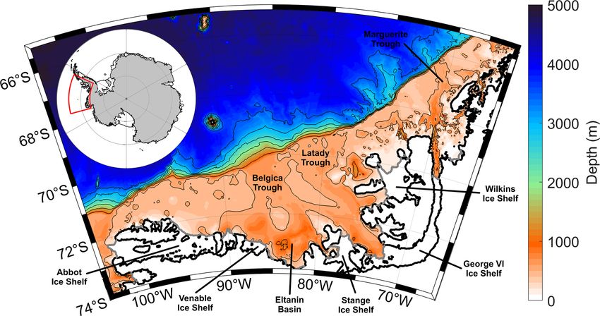
4180                                             R. Schubert et al.: The Antarctic Coastal Current in the Bellingshausen Sea

Figure 1. Bathymetry of the Bellingshausen Sea and West Antarctic Peninsula continental shelves (red box in the inset plot) as given by
the RTopo2 data product (Schaffer et al., 2016). Thin black contours delineate isobaths between 0 and 3000 m, with a 500 m interval. Thick
black and gray lines indicate the coastline and the edge of permanent ice shelves, respectively. Key geographic features are labeled.

continent. While the ASF is typically defined by a strong gra-         easterly winds piling water along the coast. The current then
dient in temperature, marked by the southernmost extent of             becomes more strongly baroclinic as meltwater is introduced
unmodified CDW (Whitworth et al., 1998), the AACC is typ-              near Marguerite Trough (Smith et al., 1999). This study also
ically characterized by a strong gradient in salinity. The first       suggested that the current could continue into the Belling-
observations of the AACC were recorded by Sverdrup (1953)              shausen Sea, but there was insufficient data to support this
in the Weddell Sea in which he noted that a westward-flowing           suggestion. Moffat et al. (2008) emphasized seasonal vari-
current split around 0◦ , with one branch continuing along the         ations in the coastal current, which they referred to as the
coastline into the Weddell Sea.                                        Antarctic Peninsula Coastal Current. We will show below
   Throughout this study, the AACC will be defined as the              that this circulation feature extends well beyond the Antarctic
current bounded on the shoreward side by either the coastline          Peninsula; hence, we will refer to this extensive coastal cur-
or the face of ice shelves. Similar to the ASC, the AACC may           rent system as the Antarctic Coastal Current (AACC). Moffat
arise in response to both surface mechanical and buoyancy              et al. (2008) argued that the AACC forms during the spring
forcing, and the relative importance of these two may impact           and summer ice-free season, and that it disappears during the
the current’s vertical structure. The AACC in the Weddell              winter when sea ice formation and a reduction in meltwa-
Sea is characterized as being primarily a barotropic current,          ter fluxes reduces lateral density gradients. The AACC has
where wind is the main factor in its barotropic variability            been studied in the Bellingshausen Sea using coupled mod-
(Núñez-Riboni and Fahrbach, 2009). Closer to the Weddell–              els and connecting the current in the WAP to the Amund-
Scotia Confluence, Heywood et al. (2004) described the                 sen Sea (Assmann et al., 2005; Holland et al., 2010). Ass-
AACC as a fast and shallow flow in the continental shelf re-           mann et al. (2005) used a coupled ice–ocean model to reveal
gion. Moffat et al. (2008) describe the coastal flow on the            a westward flow of sea ice along the coastline that is part of a
WAP as being a baroclinic current driven by strong density             large cyclonic circulation that flows from the WAP, through
gradients, generated by buoyancy input from meltwater and              the Bellingshausen Sea into the Amundsen and Ross seas.
runoff, although they also acknowledged the importance of              Sea ice drift in this model primarily occurs due to wind forc-
wind forcing. A coastal current is also found along the WAP            ing, but surface ocean currents also push the sea ice to the
in wind-forced numerical simulations controlled by the pre-            west. Holland et al. (2010), through the use of a wind forced
vailing easterly winds (Holland et al., 2010), despite the ab-         ice–ocean–atmosphere model, revealed that in summer and
sence of runoff and weak meltwater forcing. Thus, the flow             autumn a coastal current starts in the WAP and flows south-
of the AACC throughout West Antarctica and its variability             westward into the Bellingshausen Sea and exits as a strong
is linked to both wind and buoyancy forcing (Moffat et al.,            westward flow to the north of the Abbot and Venable ice
2008; Holland et al., 2010; Kim et al., 2016; Kimura et al.,           shelves. The authors speculated that this coastal current is a
2017).                                                                 continuation of the current found in Moffat et al. (2008), and
   Focusing specifically on West Antarctica, the AACC                  that it most likely continues into the Amundsen Sea (Holland
shows regional differences in its formation and maintenance.           et al., 2010).
Smith et al. (1999) described the AACC as a result of north-

The Cryosphere, 15, 4179–4199, 2021                                                         https://doi.org/10.5194/tc-15-4179-2021
R. Schubert et al.: The Antarctic Coastal Current in the Bellingshausen Sea                                                   4181

   Direct ship-based measurements of the AACC over the              strength and spatial evolution of the AACC will be consid-
continental shelf in the Bellingshausen Sea region (Fig. 1) are     ered by diagnosing dynamic height, geostrophic velocities,
limited. Jenkins and Jacobs (2008) studied the flow under the       and volume transports.
George VI Ice Shelf, noting that warm CDW floods the con-
tinental shelf, causing melting beneath the ice shelf, which
escapes to the south. There is a cyclonic circulation in each       2     Data and methods
of the major troughs in the Bellingshausen Sea, where warm
                                                                    Data collected from instrumented southern elephant seals
CDW flows shoreward along the eastern boundary of the
                                                                    provide the basis for this investigation of the physical prop-
troughs up to the ice shelves (Schulze Chretien et al., 2021).
                                                                    erties and circulation on the shelf in the Bellingshausen Sea
Subsequent ice shelf melt introduces freshwater, creating
                                                                    (Roquet et al., 2017). This study makes use of nearly 20 000
modified CDW that then flows away from the shore along
                                                                    seal profiles from the Bellingshausen Sea that were originally
the western boundary of the troughs (Zhang et al., 2016;
                                                                    analyzed by Zhang et al. (2016) and an additional 10 000 pro-
Thompson et al., 2020; Schulze Chretien et al., 2021). How-
                                                                    files that extend further to the northeast over the WAP. Fig-
ever, there have been no direct observations of the AACC in
                                                                    ure 2 shows the spatial extent of the available seal data in the
the Bellingshausen Sea. In the western Amundsen Sea, the
                                                                    Bellingshausen Sea region. The seal data span the years 2007
AACC has been identified as being a strong westward cur-
                                                                    to 2014, although there is a gap in observations between 2010
rent generated by easterly winds, with a variable baroclinic
                                                                    and 2013. Just over 22 000, or 73 % of the profiles were col-
component (Kim et al., 2016). Kimura et al. (2017) explain
                                                                    lected during “winter” months (April–September), as com-
that a high volume of meltwater is introduced from the ice
                                                                    pared to “summer” months (October–March), thus predom-
shelves in the region, establishing a strong baroclinic flow to
                                                                    inantly showing properties when sea ice covers most of the
the west. This flow then exits along the northwestern side of
                                                                    shelf. Critically, this a period when ship-based observations
the Amundsen Sea and flows towards the Ross Sea (Assmann
                                                                    in the region are almost completely unavailable.
et al., 2005; Kim et al., 2016; Kimura et al., 2017; Nakayama
et al., 2020). Through the connection between the WAP and           2.1    Southern elephant seal data
the Amundsen Sea, the presence of the AACC in the Belling-
shausen Sea has been implied, but not demonstrated, using           In this study, hydrographic data from instrumented elephant
direct observations.                                                seals are analyzed, a subset of which was previously ana-
   The AACC provides an important transport pathway that            lyzed by Zhang et al. (2016, Fig. A1). We accessed data from
connects various regional seas throughout West Antarctica           the Marine Mammals Exploring the Oceans Pole to Pole
and potentially even further to the west (Nakayama et al.,          (MEOP-CTD; Conductivity–Temperature–Depth) database
2020). The AACC may also play a key role in the overturn-           where CTD–Satellite Relay Data Loggers (CTD–SRDL) are
ing circulation over the continental shelf by modifying the         deployed on elephant seals (Roquet et al., 2013). A total of
vertical stratification. Silvano et al. (2018) showed that fresh-   29 967 hydrographic profiles were analyzed in the Belling-
water fluxes into the surface ocean stratify the upper ocean,       shausen Sea and the WAP. This represents an increase over
reducing heat loss to the atmosphere and enhancing the trans-       the 19 893 profiles analyzed by Zhang et al. (2016) due to
fer of heat to the base of ice shelves. Similar stratification      the additional data along the WAP. These data cover periods
responses and a warming of shelf waters have been high-             from 2005 to May 2006, 2007 to 2010, the austral summer of
lighted in recent numerical studies (Bronselaer et al., 2018;       2013 and 2014, and June 2015, giving it broad coverage both
Golledge et al., 2019; Moorman et al., 2020), although the          spatially and temporally. The majority of the seal dives were
full potential for feedbacks has not been explored due to ei-       collected during austral autumn and winter. Figure 2b and c
ther the coarse resolution of these simulations or their lack       show the seasonal differences in seal sampling in the Belling-
of ice shelf cavities. Flowing along the face of the major ice      shausen Sea. During summer (Fig. 2b), the seal profiles tend
shelves in West Antarctica, the AACC has an important role          to be focused near the coast and over the continental shelf,
for establishing the partitioning of vertical and lateral heat      whereas during winter (Fig. 2c), the seal profiles are more
transport and provides a key link between regional forcing          concentrated in the northeastern part of the shelf and along
and remote responses.                                               the shelf break. This is an important distinction due to the
   The purpose of this study is to investigate the horizontal       potential for seasonality in the AACC, although we note that
and vertical distribution of temperature, salinity, and density     near-coastal observations are not completely absent in winter
over the continental shelf of the Bellingshausen Sea with a         months. Throughout this study, we report the median prop-
view to mapping the structure and evolution of the AACC.            erties of the AACC using all available data. Data were pro-
Here we used hydrographic observations obtained from in-            duced for both mean and median quantities, but there were
strumented elephant seals, i.e., a data set that enables the gen-   not significant differences between the two quantities.
eration of gridded, horizontal maps of hydrographic proper-
ties. The frontal structure of the AACC is explored by creat-
ing composite hydrographic sections from the seal data. The

https://doi.org/10.5194/tc-15-4179-2021                                                  The Cryosphere, 15, 4179–4199, 2021
4182                                            R. Schubert et al.: The Antarctic Coastal Current in the Bellingshausen Sea

Figure 2. Distribution of (a) all seal data, (b) seal data in summer months (October–March), and (c) seal data in winter months (April–
September) from the Marine Mammals Exploring the Oceans Pole to Pole (MEOP-CTD) database within the Bellingshausen Sea. Contours
are the same as in Fig. 1.

   For each profile, we follow the method described in Zhang
et al. (2016) where properties are linearly interpolated onto
a vertical, nonuniform grid with 52 depth bins. All data have
undergone temperature and salinity calibration. Following
the MEOP standard, calibration was conducted based on his-
torical data in nearby regions (Roquet et al., 2011). The cali-
brated data have estimated uncertainties of ±0.02 ◦ C for tem-
perature and a ±0.02 practical salinity unit (psu) for salinity.
Additional information about data calibration can be found
in Zhang et al. (2016).

2.2    Horizontal maps

To assess the horizontal variability in the physical properties
                                                                      Figure 3. Distribution of profiles from instrumented seals used to
in the Bellingshausen Sea shelf region, the seal data were
                                                                      construct composite, cross-shelf hydrographic sections. The tran-
mapped onto a 1◦ longitude by 0.5◦ latitude grid (Fig. 4a).           sects are numbered consecutively from 1, at the most northeast-
This grid size was chosen to provide the highest resolution           ern end over the West Antarctic Peninsula shelf (see Appendix;
on the shelf, while maintaining an adequate number of grid            Fig. A1), to 7, at the western edge of the Bellingshausen Sea. Con-
cells that contain at least one data point. We note that if the       tours are the same as in Fig. 1.
AACC is narrower than our grid, then the front would look
broader than it actually is; in some regions, the AACC has
been observed to be a narrow feature of roughly 20 km (Mof-
fat et al., 2008). However, the horizontal maps, and the sub-         The other five sections are located in the Bellingshausen Sea
sequent dynamic height plot, are important for documenting            (Fig. 3). A moving median of the seal profiles was taken us-
the structure and extent of the AACC. In each grid cell, and          ing a different length scale for each section, based on the
for each depth bin, the median values of temperature and              available data. For example, in section 1, the length of the
salinity were calculated from the seal dives in that cell, as         section is 0.75◦ of latitude and the medians of the properties
well as the variance. Separate calculations for summer and            were taken every 0.075◦ of latitude. The length scale over
winter months were also completed. The dynamic height, ref-           which the median was calculated was similar across vari-
erenced to 400 m, was calculated from the median values.              ous sections but was allowed to vary to ensure that each sec-
                                                                      tion avoided gaps with unavailable data. A varying bin width
2.3    Hydrographic sections                                          did not qualitatively or quantitatively change our results. We
                                                                      chose to use degrees of latitude for convenience because the
A total of seven composite hydrographic sections, spanning            distance in kilometers is slightly different in each section.
the continental shelf break to the coast, were created to ex-         Table 1 provides details about the number of profiles, length,
amine how the vertical structure of physical properties in the        and averaging length for each of the seven sections.
Bellingshausen Sea changes from east to west. All of the                 To characterize the strength of the AACC, geostrophic ve-
sections, with the exception of section 1, have more winter           locities and transports perpendicular to each section were cal-
profiles than summer profiles, which biases the properties on         culated based on the density structure. In order to calculate
the shelf in each section towards winter values. Of the sec-          the total geostrophic velocity and transport, a reference level,
tions, two are located in the WAP to compare the seal data            or level of no motion, must be selected. A reference level of
with the AACC observations reported in Moffat et al. (2008).          400 m was applied to ensure that the full depth of the AACC

The Cryosphere, 15, 4179–4199, 2021                                                       https://doi.org/10.5194/tc-15-4179-2021
R. Schubert et al.: The Antarctic Coastal Current in the Bellingshausen Sea                                                         4183

Table 1. Length of section (degrees latitude; kilometers), number of winter (April–September), summer (October–March), total profiles, and
the averaging length (degrees latitude; kilometers) for each of the seven hydrographic sections shown in Fig. 3.

            Section    Length of section    Length of section            Bin size    Bin size     Winter    Summer        Total
            number     (degrees latitude)               (km)    (degrees latitude)      (km)     profiles    profiles   profiles
            1                       0.75                 143                0.075       14.3        183          221       404
            2                       1.15                 160                 0.05        7.0        494           67       561
            3                        1.0                 151                 0.05        7.5       1040          145      1185
            4                        1.0                 136                 0.05        6.7        753          243       996
            5                        2.7                 325                 0.15       18.1        348          168       516
            6                        4.0                 450                 0.20       22.5        117          150       267
            7                        2.5                 280                 0.25       28.0        147           59       206

was captured. This depth roughly marks the lower boundary              ter (WW), and meltwater. The temperature of AASW is di-
of the water column exhibiting significant freshwater anoma-           rectly influenced by surface heat fluxes, but the salinity of
lies that we attribute to meltwater. Some sections reveal a            AASW can be modified by a broad range of processes, in-
slight flow reversal below our reference level; however, the           cluding precipitation/evaporation, runoff from land, sea ice
bulk of the baroclinic coastal current is above this reference         formation and melt, and glacial meltwater (Meredith et al.,
level. We have opted to keep the level of no motion consis-            2013; van Wessem et al., 2017). Only the latter has a sub-
tent across all composite hydrographic sections to limit the           surface expression when it is sourced from the base of float-
impact of varying topography. In Sect. 4, we also present              ing ice shelves, and it appears as a mixture of pure meltwa-
the geostrophic transport referenced to 200 m for compari-             ter with other properties, giving rise to a glacially modified
son with the velocity structure in Moffat et al. (2008), who           version of CDW and/or WW (Fig. 5) (Castro-Morales et al.,
found a zero crossing for velocity based on shipboard acous-           2013; Schulze Chretien et al., 2021). Each of these freshwa-
tic Doppler current profiler (ADCP) data close to 200 m. Re-           ter sources have distinct isotopic signatures (Meredith et al.,
gardless of the reference level applied, the volume transport          2008) but are difficult to distinguish with the tracers provided
of the AACC was defined as the vertical integral of the ref-           by the instrumented seals. Due to these limitations, we do not
erenced geostrophic velocities between the sea surface and             explicitly discuss the distribution of meltwater fractions in
the depth of the 34.4 psu isohaline, as in Moffat et al. (2008).       this study. Recent studies of the meltwater distribution in the
In order to define the offshore extent of the AACC for each            Bellingshausen Sea can be found in Schulze Chretien et al.
section, we first found the center of the AACC by calculat-            (2021) and Ruan et al. (2021).
ing where the gradient in net transport was greatest. We then             AASW, which represents the surface mixed layer, has po-
searched in the offshore direction for the location where the          tential temperatures ranging from −1.8 to 1 ◦ C and salin-
depth-integrated velocity was 15 % of the value at the center          ity ranges from 33 to 34 psu. During austral winter, surface
of the AACC. We chose to use 15 % of the maximum value                 heat loss leads to a deeper mixed layer. In summer, surface
because it returned locations that corresponded with a level-          heating and freshening from sea ice melt restratifies the sur-
ing off of the net transport for each section.                         face ocean and leads to shallower mixed layers (Jenkins and
   To provide an estimate of the error in the velocity/transport       Jacobs, 2008; Whitworth et al., 1998). Remnant properties
calculations, we applied a bootstrapping approach (Efron and           of the wintertime deep mixed layer comprise the WW wa-
Tibshirani, 1994). Along each section, 1000 different com-             ter mass that is expressed as a temperature minimum layer
posite hydrographic sections were created by randomly se-              from −1.8 to −1.5 ◦ C and a salinity of about 34.1 psu. WW
lecting only 40 % of the profiles in each cross-shelf bin.             typically ranges from σ0 = 27.2 to 27.4 kg m−3 , where σ0 is
Geostrophic velocities and geostrophic transports were cal-            potential density referenced to the surface. Below the pyc-
culated for each of these 1000 sections, and error bars are            nocline lies CDW, which is relatively warm and salty, with
reported as the root mean square (RMS) of these values. The            values from 1 to 1.5 ◦ C and 34.7 and 34.85 psu, respectively.
RMS values are taken as the difference from the mean com-              CDW occupies the water column from the seafloor to the
posite section using all the data.                                     base of the pycnocline. Since CDW occupies a large portion
                                                                       of the water column, it is an important source of heat over
                                                                       the continental shelf and drives basal melting of ice shelves
3   Physical properties of the Bellingshausen Sea shelf                (Dutrieux et al., 2014; Schmidtko et al., 2014). Basal melting
                                                                       produces meltwater that may entrain both CDW and WW as
Water properties in the Bellingshausen Sea can be broadly              it rises along the base of ice shelves and exits the ice shelf
categorized in terms of the following four main water                  cavity. Meltwater layers have been identified in the southern
masses: Antarctic Surface Water (AASW), CDW, winter wa-

https://doi.org/10.5194/tc-15-4179-2021                                                         The Cryosphere, 15, 4179–4199, 2021
4184                                            R. Schubert et al.: The Antarctic Coastal Current in the Bellingshausen Sea

Bellingshausen Sea at depths associated with the draft of the       are associated with large polynyas (Tamura et al., 2008). Lat-
ice shelf faces (Schulze Chretien et al., 2021).                    eral changes in temperature within the coastal boundary cur-
                                                                    rent are smaller, but the trend shows a consistent cooling
3.1     Horizontal distributions                                    from east to west. Similarly, the salinity of the WW layer
                                                                    varies, freshening from east to west, both broadly over the
Due to the broad coverage of the seal profiles, this data set of-   continental shelf and in the boundary current (Fig. 4d). The
fers a unique opportunity to construct horizontal mean fields       difference in the salinity from east to west has a magnitude
that may be constructed either along isobars or isopycnals.         of roughly 0.055. This cooling and freshening signal in the
We focus on the latter in the following subsections. These          boundary current is related to an introduction of meltwater
maps provide a more complete picture of hydrographic vari-          from the ice shelves in the Bellingshausen Sea.
ations than is typically permitted from discrete hydrographic          Comparing summer and winter properties of the WW layer
sections (e.g., Castro-Morales et al., 2013). Summer melt-          reveals that there are larger horizontal gradients in sum-
ing of sea ice freshens and cools the surface layers, which,        mer compared to the winter months (Fig. A2). Temperature,
combined with heating later in the summer, forms the fresher        salinity, and isopycnal layer depth all have larger lateral gra-
and warmer seasonal thermocline. In the winter, sea ice for-        dients in summer than in winter in the region from 70◦ W
mation increases salinity through brine rejection, resulting        to the George IV inlet. The temperature, on average, along
in mixing and deepening of the mixed layer. Thus, AASW              the western front of the Wilkins Ice Shelf is roughly 0.2 ◦ C
shows the most variability in properties due to seasonal sur-       higher in winter than in summer, and the salinity is roughly
face forcing variations (Whitworth et al., 1998). Our focus         0.015 psu greater in the winter than in the summer. The depth
in the following is on layers below the surface, or water           of the WW layer only varies by about 10 m between winter
masses below AASW. We define these water masses based               and summer. The smaller gradients from east to west in the
on density surfaces, which slightly differ over the span of the     winter could result from weaker advection from the AACC in
Bellingshausen Sea, to support our goal of describing how           the WAP. Moffat et al. (2008) defined the AACC as a strong
the properties change along the path of the AACC.                   coastal current in the summer, which weakens in winter. The
                                                                    AACC would provide an influx of warm, salty water into
3.1.1    Winter water                                               the Bellingshausen Sea in the summer, which would tend to
                                                                    strength gradients in summer, as compared to winter.
We illustrate the properties of the WW layer on the σ0 =
27.4 kg m−3 surface (Fig. 4b–d), with median values of              3.1.2   Transitional layer
isopycnal layer depth, temperature, and salinity taken from
all available seal data. Properties of the continental shelf have   On the σ0 = 27.65 kg m−3 layer that lies between the WW
been removed in panels (b–d) to better highlight variations         and CDW layers, the water is a mixture of WW, CDW, and
over the continental shelf. Seasonal variations in the WW           glacial meltwater (Fig. A3). This layer roughly aligns with
properties (divided into 6-month periods) are provided in the       the pycnocline and the base of the AACC; thus, it is impor-
Appendix (Fig. A2). A key feature of the WW layer is its            tant to document its evolution along the coast. The horizontal
downward slope along the entire coast of the Bellingshausen         gradient in isopycnal depth, perpendicular to the coast, has a
Sea, indicating a baroclinic, westward geostrophic current,         similar pattern to this gradient in the WW layer. In the eastern
under the assumption that the velocity decays with depth            Bellingshausen Sea, it is narrow and progressively becomes
(Fig. 4b). The shape of the 27.4 kg m−3 surface highlights          wider as the AACC moves along the Wilkins Ice Shelf. In
the boundary-trapped nature of the AACC up to the west-             the central Bellingshausen Sea, it again becomes narrow, but
ern limit of the Bellingshausen Sea shelf, where the deeper         the magnitude increases before becoming wider again as the
excursion of the isopycnal surface extends away from the            AACC exits the western Bellingshausen Sea. The potential
coast toward the shelf break. The offshore spatial gradient         temperature of the transitional layer (Fig. A3b) is warmer
in the depth of the WW layer, calculated perpendicular to           than the overlying WW layer, with warmer water in the east
the coastline, appears as a narrow and relatively weak gradi-       and colder water in the west, although the change in tem-
ent in the east. The isopycnal depth gradient widens, and its       perature from 70◦ W to the entrance of the George VI Ice
magnitude increases south of the Wilkins Ice Shelf and into         Shelf is not as strong as for the WW layer, with a magnitude
the central Bellingshausen Sea. The region of isopycnal tilt        of roughly 0.54 ◦ C. Instead, this layer has a more consistent
broadens again to the west in front of Abbot Ice Shelf. The         shift to colder waters in the west. Salinity is higher in the
potential temperature of the WW layer (Fig. 4c) is consider-        east, at about 34.65, and transitions to lower values in the
ably warmer in the eastern Bellingshausen Sea as compared           west, at about 34.61.
to the west, with a difference of roughly 1.15 ◦ C.                     The differences between summer and winter months for
   Close to the coast, the temperature on this density surface      the transition layer are similar to the WW layer (Fig. A3d–
is warmer than what is typically associated with WW, which          i). The temperature shows larger gradients in the Wilkins Ice
may be due to upward mixing of warm CDW, as these regions           Shelf region in summer compared to winter. The larger gra-

The Cryosphere, 15, 4179–4199, 2021                                                    https://doi.org/10.5194/tc-15-4179-2021
R. Schubert et al.: The Antarctic Coastal Current in the Bellingshausen Sea                                                              4185

Figure 4. Mean spatial distribution of winter water (WW) properties in the Bellingshausen Sea. The map is constructed using a grid spacing
of 0.5◦ latitude and 1◦ longitude. (a) The number of data points within each grid cell (white represents a grid cell with no data). (b–d) Depth
(meters), potential temperature (degrees Celsius), and salinity, respectively, on the 27.4 kg m−3 isopycnal.

Figure 5. Potential temperature–salinity plots as measured by instrumented seals in the Bellingshausen Sea. (a) A two-dimensional histogram
of all the seal data over the continental shelf, using salinity and temperature intervals of 0.02 psu and 0.02 ◦ C, respectively. The scale is
logarithmic. (b) The distribution of potential temperature and salinity from the composite hydrographic sections is listed in Table 1. The thin
black contour lines are of potential density. The thick black line is the freezing line.

dient in summer is due to warmer temperatures in the east,                isopycnal slopes down towards the coast, similar to the WW
at around 72◦ W, compared to winter. In the east, the salinity            and transitional layers (Fig. A4a). As in the other layers, this
gradients are larger in the summer than in the winter, where              change in the depth of the isopycnal layer is much broader in
the salinity in the east is higher in summer compared to win-             the western Bellingshausen Sea, as compared to the central
ter. The property changes between seasons are less clear far-             and eastern regions. The potential temperature in this layer is
ther to the west due to a lack of seal data.                              warmer and less variable than the overlying layers (Fig. A4),
                                                                          with a difference from east to west of only 0.22 ◦ C. However,
3.1.3   Circumpolar deep water                                            there is a large-scale spatial distribution with warmer waters
                                                                          in the east and cooler waters in the west. The modification of
Properties of the CDW layer are given by values interpo-                  temperature and salinity within the boundary current is less
lated onto the σ0 = 27.75 kg m−3 isopycnal (Fig. A4). This

https://doi.org/10.5194/tc-15-4179-2021                                                          The Cryosphere, 15, 4179–4199, 2021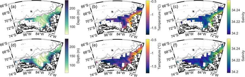
4186                                            R. Schubert et al.: The Antarctic Coastal Current in the Bellingshausen Sea

evident in the CDW layer as compared to the WW and tran-            Sea. This section is also located west of Marguerite Trough
sitional layers, which again highlights the likely importance       (Fig. 3, a key route for warm CDW to access the continental
of meltwater leaving the ice shelf cavities at depths shallower     shelf and the northern extent of the George IV Ice Shelf (Ven-
than CDW (Schulze Chretien et al., 2021). A similar pattern         ables et al., 2017; Brearley et al., 2019). In the composite
can be seen in salinity, with saltier waters in the east and        section, the surface temperature varies only slightly from the
fresher waters in the west (Fig. A4), and a difference between      coast to the shelf break (Fig. 6c), with an average tempera-
these two regions of roughly 0.019. The near-absence of lo-         ture of −1.5 ◦ C. In contrast to temperature, the surface salin-
calized variability along the coast suggests that the AACC is       ity (Fig. 6c) shows substantial lateral variations along sec-
less of a factor in water modification in this layer.               tion 3, with a shallow fresh layer that extends from the coast
   The CDW layer does not show notable differences be-              to roughly 68.6◦ S, increasing from 33.7 psu near the coast to
tween winter and summer months, consistent with this layer          34 psu near the shelf break. Below this surface layer, the ver-
being largely isolated from surface forcing. In the east, the       tical (composite) stratification peaks at roughly 150 m depth.
temperature in summer is slightly cooler than in winter; how-       The vertical stratification is set by the salinity as temperature
ever, the gradients from east to west are of similar magnitude      increases almost uniformly throughout the water column, in-
in both times of the year. Salinity variations between winter       creasing from −1.4 ◦ C above the halocline to 0.5 ◦ C below
and summer are even weaker than temperature, although we            the halocline. At the shelf break, near 68◦ S, a warm core of
note that the comparison of seasonal property changes in the        CDW is found between 250 and 500 m, with temperatures
western region of the Bellingshausen Sea is difficult due to        exceeding 1.5 ◦ C. This structure is consistent with warm wa-
the lack of observations in winter.                                 ters observed over the shelf modified from offshore sources
                                                                    through some combination of mixing processes, surface forc-
3.2    Vertical distributions                                       ing, and interactions with ice shelves.
                                                                       Isopycnals are aligned with salinity contours and are
The composite hydrographic sections across the shelf of the         nearly flat offshore of 68.4◦ S. Onshore of this latitude, the
Bellingshausen Sea are used next to display the median verti-       salinity and the density contours slope down towards the
cal structure of hydrographic properties. The overall vertical      coast. This downward tilt of the isopycnals is a common fea-
structure in each section is similar, starting with a more vari-    ture across all the composite sections and gives rise to the
able surface water layer, then a WW layer characterized by          baroclinic structure of the AACC flowing southwestward in
a temperature minimum, and below that a warm CDW layer              the WAP and westward in the Bellingshausen Sea.
that extends to the seafloor. Surface temperatures along each          The easternmost section (section 1; Fig. 6a) shows two
of the composite sections in the Bellingshausen Sea vary            near-surface cores of warm water with temperatures exceed-
only slightly from the coast to the shelf break, whereas there      ing 1 ◦ C. These cores are bounded by colder waters where the
is greater variability in surface temperatures in the eastern       surface approaches the freezing temperature. Section 1 is the
composite sections over the WAP continental shelf. Surface          only composite section where summertime profiles exceed
salinity variations are similar over both the Bellingshausen        the number of wintertime profiles, which is why surface tem-
Sea and the WAP continental shelves, showing fresher wa-            peratures are warmer than other sections. The salinity shows
ter near the coast and saltier water near the shelf break. In       surface variations, initially fresher at 34 psu and increasing
total, seven hydrographic sections were constructed to show         to 34.2 psu at the first temperature minimum. The potential
the evolution of properties and transports along the ice shelf      density contours of 27.3 and 27.4 kg m−3 extend towards the
front (Fig. 3). Note the change in scale for the different pan-     surface (Fig. 6a) at the temperature minima. This structure
els, to span the different distances, with the along-section dis-   is likely a remnant of winter ice freezing on the shelf. Be-
tance indicated above the potential temperature. The 34.4 psu       low the surface layer, the temperature is more uniform across
isohaline is also included in the geostrophic velocity panels       the shelf and shelf break compared to hydrographic section 3
in Fig. 9.                                                          (Fig. 6a). Beneath the thermocline, the temperature is close
   We used all available data for each composite section.           to 1.3 ◦ C across the entire section, increasing to about 1.5 ◦ C
Since there are considerably more data from winter months,          at the bottom. Salinity increases from 34.5 psu at the top of
the properties are more strongly weighted to winter seasons.        the halocline to 34.7 psu at the bottom of the halocline. The
For this reason, the distinction between AASW and WW wa-            salinity reaches a maximum of roughly 34.8 psu at the bot-
ter masses in each section is reduced. We begin by providing        tom. Density follows the salinity and slopes down towards
a detailed discussion of hydrographic section 3, which marks        the coast near 65.55◦ S. This structure is similar to the hy-
the eastern boundary of the Bellingshausen Sea and is largely       drographic sections presented in Moffat et al. (2008).
representative of the other sections. For subsequent sections,         Hydrographic section 2 (Fig. 6b) shows structure more
we mainly highlight key differences from hydrographic sec-          typical of the water column over the rest of the shelf. The
tion 3.                                                             surface mixed layer, consisting of AASW and WW, shows
   Hydrographic section 3 (Fig. 6c) marks the boundary be-          a temperature minimum from about 67.25◦ S to the north-
tween the WAP continental shelf and the Bellingshausen              ern extent of the section. From 67.25◦ S, the temperature in-

The Cryosphere, 15, 4179–4199, 2021                                                     https://doi.org/10.5194/tc-15-4179-2021
R. Schubert et al.: The Antarctic Coastal Current in the Bellingshausen Sea                                                           4187

Figure 6. Vertical hydrographic sections of potential temperature (top) and salinity (bottom) in the upper 700 m for each section in Fig. 3.
Distance along the section is provided along the top of the temperature panels; note that sections are not of equal length.

https://doi.org/10.5194/tc-15-4179-2021                                                        The Cryosphere, 15, 4179–4199, 2021
4188                                            R. Schubert et al.: The Antarctic Coastal Current in the Bellingshausen Sea

creases from −1.8 to −1.28 ◦ C at the coast. Near the coast         height is elevated near the coast throughout the Belling-
the salinity is 33.71 psu and increases to 34.1 psu at 67.25◦ S.    shausen Sea (Fig. 8), consistent with a pressure gradient di-
North of this latitude, the salinity varies between 34.1 and        rected offshore, and balanced by the Coriolis force to support
34.2 psu, with maximum values close to the shelf edge. The          a mean, near-surface, westward, along-coast flow. This flow
thermocline and halocline occur around 125 m depth. The             is discussed in more detail below by constructing compos-
temperature profile beneath the thermocline increases to an         ite sections of geostrophic velocity (Fig. 9). In the eastern
average maximum temperature of 1.4 ◦ C at 400 m. Pockets of         Bellingshausen Sea, dynamic height indicates that a coastal
warmer water exist in cores around 400 m, reaching 1.52 ◦ C.        flow enters from the WAP as a narrow boundary current.
The salinity below the halocline increases from about 34.65         The value is largest near the coast and changes by 0.6 m2 s−2
to 34.75 psu at the bottom. The density on level surfaces de-       across an offshore distance of roughly 100 km. As the AACC
creases towards the coast at roughly 67.25◦ S, indicating the       flows around the Wilkins Ice Shelf, the region of strong
presence of the AACC.                                               dynamic height gradient widens to 140 km, but the differ-
   Moving west of section 3, into the Bellingshausen Sea            ence in dynamic height increases to 0.8 m2 s−2 . In the central
shelf region, the temperature near the surface appears              Bellingshausen Sea, the region of strong dynamic height gra-
warmer, particularly near the coast. The salinity at the sur-       dient becomes narrower, occupying a region of only 70 km,
face progressively decreases, and this fresher water extends        and the difference in dynamic height across this boundary
farther away from the coast. We believe that this occurs due        current continues to increase to 0.9 m2 s−2 . Here the veloc-
to the continued entrainment of meltwater by the AACC from          ity of the AACC has its greatest magnitude in the Belling-
the melting ice shelves (Schulze Chretien et al., 2021). The        shausen Sea. The difference in dynamic height across the
thermocline and halocline are found at somewhat deeper lev-         boundary current continues to increase through the Venable
els, from a depth of 150 m in section 3 to a depth of 200 m in      Ice Shelf, until, on its western side, the region of strong gra-
section 7. The isopycnal tilt near the coast strengthens some-      dient widens to over 200 km with a difference of 0.8 m2 s−2 .
what from east to west but, more importantly, extends to a          West of the Venable Ice Shelf, the dynamic height contours
greater distance away from the coast, indicating that the baro-     suggest that the path of the AACC divides, with some com-
clinic portion of the AACC intensifies (Sect. 4).                   ponent of the flow directed toward the shelf break and an-
   The vertical structure of properties is important for un-        other component along the face of the Abbot Ice Shelf.
derstanding the evolution of the AACC. At the surface, the             We next use the composite hydrographic sections to con-
temperature becomes slightly warmer near the coast, but the         struct geostrophic velocities perpendicular to the section and,
most noticeable change is a reduction in salinity, which has        therefore, largely oriented parallel to the shelf break and the
a larger effect on density. The thermocline and halocline are       coastline. Figure 9 shows the geostrophic velocity and cumu-
depressed and found deeper in the west compared to in the           lative volume transport for each of the hydrographic sections
east. The vertical stratification near the coast also undergoes     (negative values are directed westward). The transport is cal-
an evolution from east to west (Fig. 7). Over the WAP shelf         culated by integrating the velocities with respect to depth be-
(sections 1–3), the stratification, given in terms of the buoy-     tween the 34.4 isohaline and the surface and with distance
ancy frequency N 2 = −g/ρ0 (dρ/dz), where g is gravity, and         from the coast, such that the transport at the outer limit is
ρ0 = 1027 kg m−3 is a reference density, peaks at a value of        equivalent to the net along-shelf volume transport in Sver-
2 × 10⁻⁵ s−2 at a depth of 150 m. Once entering the Belling-        drups (1 Sv = 106 m3 s−1 ). Table 2 summarizes the results
shausen Sea, the AACC stratification changes in two im-             for each of the seven hydrographic sections.
portant ways; first, the near-surface (upper 100 m) becomes            In order to arrive at an absolute geostrophic velocity, a ref-
much more stratified, and the stratification deepens with N 2       erence level of no motion must be selected. Here, we apply
exceeding 2 × 10⁻⁵ s−2 below 300 m in sections 6 and 7              a 200 m reference level of no motion to calculate the vol-
(Fig. 7). The increase in surface stratification due to fresh-      ume transports for sections 1–3 and compare these to the
ening points to an influx of freshwater either from runoff,         volume transport calculated by Moffat et al. (2008), located
sea ice melt, or buoyant meltwater convection near the face         between sections 1 and 2, and shown in Fig. 10a. Section 1
of ice shelves. The deeper change in the stratification is likely   (Figs. 3 and 10a), located to the north and east of the Mof-
due to the outflow of glacially modified CDW and marks the          fat et al. (2008) section, has a transport of −0.26 ± 0.014 Sv.
base of the AACC (Ruan et al., 2021; Schulze Chretien et al.,       Recall that these transports represent the flow confined to the
2021).                                                              AACC as determined by the location where depth-integrated
                                                                    velocity is 15 % of the value at the center of the current (see
                                                                    Sect. 2.3 and the vertical dashed lines in Fig. 9). Section 2 is
4   Transport                                                       located to the south and west of the Moffat et al. (2008) sec-
                                                                    tion, and the transport is −0.38 ± 0.023 Sv. For comparison,
From the hydrographic data discussed in Sect. 3, a dynamic          the transport of the Moffat et al. (2008) section was reported
height field was constructed in the Bellingshausen Sea, show-       to be −0.32 ± 0.13 Sv. Moving along the coast to the west,
ing the surface values relative to 400 m depth. Dynamic             volume transports increase. Jenkins and Jacobs (2008) found

The Cryosphere, 15, 4179–4199, 2021                                                     https://doi.org/10.5194/tc-15-4179-2021
R. Schubert et al.: The Antarctic Coastal Current in the Bellingshausen Sea 4189
Figure 7. Vertical profiles of density stratification N 2 , averaged across the AACC, for the seven composite sections in Fig. 3. The sections
are arranged from east (left) to west (right).
Table 2. Width (kilometers), mean depth (meter), range of depth (meters) and along-shore transport for the AACC in each of the seven
hydrographic sections shown in Fig. 3.
Section Width of Mean depth Depth range Along-shore
number AACC (km) (m) (m) transport (Sv)
1 28.4 125.7 108–161 −0.41
2 23.8 137.3 109–161 −0.43
3 75.1 164.6 117–215 −1.55
4 60.9 193.9 143–230 −1.09
5 89.8 184.3 109–254 −2.19
6 160.9 183.6 92–230 −1.70
7 111.9 218.0 158–267 −1.89
that a transport of −0.24 Sv flows south through the Mar-
guerite Trough. This additional transport explains a jump in
transport between our sections 2 and 3, where, in the latter
section, the AACC transport is −1.0 ± 0.033 Sv. The com-
parison with the estimate from Moffat et al. (2008), using a
200 m reference level, gives us confidence that our velocity
and transport estimates are reasonable. For the remainder of
the section, we will report geostrophic velocities and trans-
ports using a 400 m reference level, as discussed in Sect. 2.3.
Throughout the WAP and Bellingshausen Sea there is
westward flow along the coast. The extent of the AACC
is defined as the region between the coast and the location
where depth-integrated velocity is 15 % of the value at the
Figure 8. Spatial map of surface dynamic height (square meters center of the current, indicated by the vertical dashed lines
per second; m2 s−2 ), referenced to 400 m. The red contours have an in Fig. 9. In section 1, the geostrophic velocity in the AACC
interval of 0.2 m2 s−2 . has a peak value of −0.21 m s−1 and an average velocity of
−0.06 m s−1 . Section 2, similarly, shows the AACC tightly
https://doi.org/10.5194/tc-15-4179-2021 The Cryosphere, 15, 4179–4199, 20214190 R. Schubert et al.: The Antarctic Coastal Current in the Bellingshausen Sea Figure 9. Geostrophic velocity (meters per second – m s−1 ; referenced to 400 m; top) and geostrophic transport (Sv; bottom) for all sections in Fig. 3. Transport values are given for both the 200 and 400 m reference level, and transports are cumulative from the coast and calculated by integrating from the surface to the 34.4 psu isohaline (red dashed curve). Negative (positive) values indicate westward (eastward) transport and flow. The Cryosphere, 15, 4179–4199, 2021 https://doi.org/10.5194/tc-15-4179-2021
R. Schubert et al.: The Antarctic Coastal Current in the Bellingshausen Sea                                                             4191

Figure 10. (a) Location of AACC transport estimates based on the hydrographic transects labeled as in Fig. 3, and (b) the values of transport
(Sv; 1 Sv = 106 m3 s−1 ) along the AACC. The transport increases as the AACC flows westward. The transport estimate from Moffat et al.
(2008) in the WAP is included in both panels and indicated by the red dot labeled M. All of the transport values, except for the Moffat et al.
(2008) section, are with respect to a level of no motion at 400 m. The red dashed line shows a linear trend of 2 Sv per 1000 km. The blue dots
in panel (a) indicate the midpoint of the AACC in each section.

confined to the coast, with a similar peak westward veloc-               transport of the boundary current at the bottom is zero (Lentz
ity of −0.20 m s−1 and an average of −0.057 m s−1 . The                  and Helfrich, 2002). If the current moves offshore to follow
peak velocities in sections 1 and 2 are similar to the sur-              a particular isobath, the AACC would appear wider, even if
face velocities found in the fall by the mooring in (Mof-                the core remains narrow (e.g., section 4). The along-coast
fat et al., 2008), which they found to range from −0.15                  transport, on the other hand, provides a clearer picture of the
to −0.20 m s−1 . Across section 3, the first section in the              evolution of the AACC. The striking feature is a nearly linear
Bellingshausen Sea, the velocity of the AACC has an av-                  trend in volume transport extending from the WAP through
erage value of −0.056 m s−1 , with a maximum value of                    the western Bellingshausen Sea. Values along the WAP show
−0.26 m s−1 . Here, the AACC occupies a much larger area                 that the AACC carries roughly 0.5 Sv of transport, which in-
than in the previous sections (Fig. 9c). In section 4, the av-           creases to more than 1 Sv in the eastern Bellingshausen Sea
erage velocity decreases to −0.04 m s−1 , and the maximum                and is ultimately close to 2 Sv in the western Bellingshausen
velocity is −0.26 m s−1 . The decrease in average velocity in            Sea (Fig. 10). Using a Monte Carlo error analysis, we also
section 4 is associated with the current splitting into three            estimated error bars for the transport (shown as vertical bars
different cores seen in Fig. 9d. As the AACC enters into the             in Fig. 10), supporting the presence of a significant trend.
central Bellingshausen Sea, the average velocity increases, in              Throughout the Bellingshausen Sea continental shelf, the
section 5, to −0.05 m s−1 . The velocity maximum in this sec-            density structure near the coast is consistent with a baro-
tion is −0.20 m s−1 , which is a decrease in magnitude from              clinic, vertically sheared flow that is westward near the sur-
the previous two sections. The next section sees the average             face. Additionally, the lateral density gradients intensify and
velocity decrease to −0.026 m s−1 and a maximum velocity                 extend further away from the coast as the AACC moves to-
of −0.11 m s−1 . The final section, section 7 in the western             wards the west, suggesting a strengthening of the AACC.
Bellingshausen Sea, has an average velocity of −0.041 m s−1              Thus, the evolution of the AACC, inferred from hydro-
and a maximum of −0.12 m s−1 . As we discuss below, part                 graphic properties through dynamic height, geostrophic ve-
of the variability in the average geostrophic velocity is tied           locity, and transport estimates, shows a consistent picture of
to a broadening of the AACC that is better captured by the               a connected circulation feature that extends from the WAP
changing geostrophic transport.                                          through the western Bellingshausen Sea.
   The magnitude of the geostrophic velocity is variable
across the various composite sections, which could result
from a number of factors, including surface forcing effects              5    Discussion
(modifying the sea surface height) and width of the AACC.
Note that the “average” velocity across the AACC, reported               The Bellingshausen Sea region shows higher salinities and
above, was selected as a simple diagnostic of the flow and               temperatures in the east near the surface, whereas, toward
should be interpreted with some caution. Even with the weak              the west, both temperature and salinity decrease. This change
stratification of the waters on the Antarctic continental shelf,         can be attributed to the following two processes: (i) the en-
the AACC may be tied to flow over particular isobaths as                 hanced basal melting in the ice shelf cavities of the Belling-
it reaches a geostrophic equilibrium where offshore Ekman                shausen Sea that produces more meltwater, and (ii) the cir-

https://doi.org/10.5194/tc-15-4179-2021                                                          The Cryosphere, 15, 4179–4199, 2021
4192 R. Schubert et al.: The Antarctic Coastal Current in the Bellingshausen Sea
culation in the AACC and the accumulation of meltwater as
the AACC flows westward. The basal melt rates of Belling-
shausen Sea ice shelves are amongst the highest throughout
Antarctica (Paolo et al., 2015; Walker and Gardner, 2017;
Adusumilli et al., 2020), which introduces meltwater mix-
tures with a lower temperature and salinity. Polynyas, asso-
ciated with brine rejection due to sea ice formation, persist
almost year round but do not lead to penetrative convection to
the seafloor (Tamura et al., 2008; Holland et al., 2010). How-
ever, there is not an accompanying increase in salinity from
east to west that would be associated with accumulating brine
rejection in areas of sea ice formation. The increased salin-
ity from ice formation in polynyas, where they are present,
counteracts to some extent the decrease seen in salinity from Figure 11. Drifter tracks for two drifters released as part of the Long
east to west. But this effect is overwhelmed by the entrain- Term Ecological Research (LTER) program and offering additional
support that the AACC provides a connection between the WAP
ment of glacial meltwater. Local sea ice variability may also
and the Amundsen Sea. Drifter 54 160 was released on 1 January
play a factor in modifying the properties of the water through
2007 and recorded positions through 24 December 2007. Drifter
ocean–atmosphere heat fluxes (Walker and Gardner, 2017). 70 579 recorded positions between 27 January and 24 November
The density field is consistent with a dominant baroclinic 2007; there is a gap in the data for this drifter during 18–27 May
structure of the AACC. The geostrophic velocities in Fig. 9 (around 74◦ W). Large black dots indicate the beginning and end of
provide details of the AACC flow. As the AACC transitions each drifter track.
from the WAP to the Bellingshausen Sea, the transport in-
creases as the warm water below the current enters the ice
cavity and produces meltwater, creating a plume of entrained ployed on 1 January 2007 and reached the central Belling-
CDW which, in turn, feeds the along-shore flow. The aver- shausen Sea, defined here as 82.5◦ W, on 15 March with
age velocity of the AACC remains relatively constant in the an average speed over that time span of 0.30 m s−1 . This
transition from the WAP to the eastern Bellingshausen Sea. drifter then reached the Abbot Ice Shelf, defined as crossing
Within the central and western Bellingshausen Sea, the av- 91.5◦ W, on 28 March. The average speed of drifter 54 160
erage velocity varies from section to section, but a widening during this stretch of time was 0.41 m s−1 . The drifter then
of the AACC causes the transport to steadily increase. Wind entered into the Amundsen Sea, providing at least anecdotal
forcing may also influence the AACC structure and is cou- evidence that the AACC in the Bellingshausen Sea is con-
pled to the presence of almost year-round polynyas near the nected to the Amundsen Sea. The last recording for drifter
coast (Assmann et al., 2005; Holland et al., 2010). However, 54 160 was on 24 December in the Amundsen Sea. From
the strength and orientation of the wind stress close to the 28 March to 24 December, the average speed was 0.22 m s−1 .
coast is not well determined due to the lack of observations Drifter 70 579, in red, was released near the coast on the
to validate reanalysis products. The introduction of meltwa- WAP on 21 January 2007 and then entered into the eastern
ter from the melting ice shelves is the most likely explanation Bellingshausen Sea, defined as crossing 71◦ W, on 9 March
for the growing transport of the AACC, consistent with the with an average velocity of 0.38 m s−1 over that time span.
observed along-coast trends in temperature and salinity. There was a gap in the drifter data between 18 and 27 May,
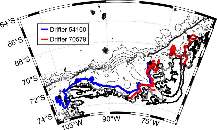
Independent evidence provided by surface drifters pro- but the velocity between the two data points that are on ei-
vides further support for a continuous coastal current ther side of the gap was 0.15 m s−1 . The final data point for
that spans the Bellingshausen Sea; surface drifter trajec- drifter 70 579 is 24 November in the central Bellingshausen
tories were also key in early studies that identified the Sea. The average velocity from 27 May to 24 November was
AACC along the WAP (Beardsley et al., 2004). Fig- 0.26 m s−1 . It is notable that these drifters persisted for nearly
ure 11 shows the tracks of two surface drifters that 12 months, suggesting that an open-water pathway along the
were released in 2007 as part of the Long Term Eco- coast is maintained over much of the year.
logical Research (LTER) program (https://scienceweb.whoi. The AACC could have as many as three separate pathways
edu/coastal/LTER_Drifter/index.html, last access: 4 Febru- from the Bellingshausen Sea into the Amundsen Sea. First,
ary 2021). Both of these drifters show a westward flow pat- near the Venable Ice Shelf and the eastern extent of the Ab-
tern consistent with a continuous AACC. These drifters pro- bot Ice Shelves, a branch of the AACC appears to deflect to
vided high-frequency position fixes with a separation of only the north, likely steered by topography on the western side
about 27 min; we have not averaged the data. Drifter 54 160, of the Belgica Trough, and flows offshore where it eventu-
(blue curve in Fig. 11) was released in the eastern Belling- ally joins the ASF. Observations over the continental shelf
shausen Sea and was advected into the eastern Amundsen and slope suggest that this is the primary route for the ex-
Sea before it stopped sending back data. This drifter was de- port of meltwater from the Bellingshausen Sea (Thompson
The Cryosphere, 15, 4179–4199, 2021 https://doi.org/10.5194/tc-15-4179-2021You can also read