SOIL-RELATED DEVELOPMENTS OF THE BIOME-BGCMUSO V6.2 TERRESTRIAL ECOSYSTEM MODEL - GMD
←
→
Page content transcription
If your browser does not render page correctly, please read the page content below
Geosci. Model Dev., 15, 2157–2181, 2022
https://doi.org/10.5194/gmd-15-2157-2022
© Author(s) 2022. This work is distributed under
the Creative Commons Attribution 4.0 License.

Soil-related developments of the Biome-BGCMuSo v6.2 terrestrial
ecosystem model
Dóra Hidy1,2 , Zoltán Barcza1,3,4 , Roland Hollós3,5,9 , Laura Dobor1,4 , Tamás Ács6 , Dóra Zacháry7 , Tibor Filep7 ,
László Pásztor8 , Dóra Incze3 , Márton Dencső8,9 , Eszter Tóth8 , Katarína Merganičová4,10 , Peter Thornton11 ,
Steven Running12 , and Nándor Fodor4,5
1 Excellence   Center, Faculty of Science, ELTE Eötvös Loránd University, 2462 Martonvásár, Hungary
2 MTA-MATE       Agroecology Research Group, Department of Plant Physiology and Plant Ecology,
Hungarian University for Agriculture and Life Sciences, 2100 Gödöllő, Hungary
3 Department of Meteorology, Institute of Geography and Earth Sciences,

ELTE Eötvös Loránd University, 1117 Budapest, Hungary
4 Faculty of Forestry and Wood Sciences, Czech University of Life Sciences Prague, 165 21 Prague, Czech Republic
5 Centre for Agricultural Research, Agricultural Institute, 2462 Martonvásár, Hungary
6 Department of Sanitary and Environmental Engineering, Budapest University of Technology and Economics,

1111 Budapest, Hungary
7 Geographical Institute, Research Centre for Astronomy and Earth Sciences, 1112 Budapest, Hungary
8 Institute for Soil Sciences, Centre for Agricultural Research, 1022 Budapest, Hungary
9 Doctoral School of Environmental Sciences, ELTE Eötvös Loránd University, 1117 Budapest, Hungary
10 Department of Biodiversity of Ecosystems and Landscape, Institute of Landscape Ecology,

Slovak Academy of Sciences, 949 01 Nitra, Slovakia
11 Climate Change Science Institute/Environmental Sciences Division, Oak Ridge National Laboratory,

Oak Ridge, TN 37831, USA
12 Numerical Terradynamic Simulation Group, Department of Ecosystem and Conservation Sciences University of Montana,

Missoula, MT 59812, USA

Correspondence: Dóra Hidy (dori.hidy@gmail.com)

Received: 26 November 2021 – Discussion started: 8 December 2021
Revised: 4 February 2022 – Accepted: 10 February 2022 – Published: 15 March 2022

Abstract. Terrestrial biogeochemical models are essential          soil hydrology as well as the soil carbon and nitrogen cy-
tools to quantify climate–carbon cycle feedback and plant–         cle calculation methods are described in detail. Capabilities
soil relations from local to global scale. In this study, a the-   of the Biome-BGCMuSo v6.2 model are demonstrated via
oretical basis is provided for the latest version of the Biome-    case studies focusing on soil hydrology, soil nitrogen cycle,
BGCMuSo biogeochemical model (version 6.2). Biome-                 and soil organic carbon content estimation. Soil-hydrology-
BGCMuSo is a branch of the original Biome-BGC model                related results are compared to observation data from an ex-
with a large number of developments and structural changes.        perimental lysimeter station. The results indicate improved
Earlier model versions performed poorly in terms of soil           performance for Biome-BGCMuSo v6.2 compared to v4.0
water content (SWC) dynamics in different environments.            (explained variance increased from 0.121 to 0.8 for SWC
Moreover, lack of detailed nitrogen cycle representation           and from 0.084 to 0.46 for soil evaporation; bias changed
was a major limitation of the model. Since problems as-            from −0.047 to −0.007 m3 m−3 for SWC and from −0.68
sociated with these internal drivers might influence the fi-       to −0.2 mm d−1 for soil evaporation). Simulations related to
nal results and parameter estimation, additional structural        nitrogen balance and soil CO2 efflux were evaluated based
improvements were necessary. In this paper the improved            on observations made in a long-term field experiment un-

Published by Copernicus Publications on behalf of the European Geosciences Union.
2158                  D. Hidy et al.: Soil-related developments of the Biome-BGCMuSo v6.2 terrestrial ecosystem model

der crop rotation. The results indicated that the model is         requires mathematical representation in models (Martínez-
able to provide realistic nitrate content estimation for the       Vilalta et al., 2016). Simulation of land surface hydrology in-
topsoil. Soil nitrous oxide (N2 O) efflux and soil respiration     cluding evapotranspiration is typically handled by some vari-
simulations were also realistic, with overall correspondence       ant of the Penman–Monteith equation that is widely studied
with the observations (for the N2 O efflux simulation bias         and thus represents a separate scientific field (McMahon et
was between −0.13 and −0.1 mg N m−2 d−1 , and normal-              al., 2013; Doležal et al., 2018).
ized root mean squared error (NRMSE) was 32.4 %–37.6 %;               Putting it all together, if we are about to construct and
for CO2 efflux simulations bias was 0.04–0.17 g C m−2 d−1 ,        further improve a biogeochemical model to consider novel
while NRMSE was 34.1 %–40.1 %). Sensitivity analysis and           findings and track global changes, we need comprehensive
optimization of the decomposition scheme are presented to          knowledge that integrates many, almost disjunct scientific
support practical application of the model. The improved ver-      fields. Clearly, transparent and well-documented develop-
sion of Biome-BGCMuSo has the ability to provide more              ment of a biogeochemical model is of high priority but is
realistic soil hydrology representation as well as nitrifica-      challenging from the very beginning and requires coopera-
tion and denitrification process estimation, which represents      tion of researchers from various scientific fields.
a major milestone.                                                    Continuous model development is inevitable, but it has
                                                                   to be supported by extensive comparison with observations
                                                                   and some kind of implementation of the model–data fusion
                                                                   approach (Keenan et al., 2011). It is well documented that
1   Introduction                                                   structural problems might trigger incorrect parameter estima-
                                                                   tion that might be associated with distorted internal processes
The construction and development of biogeochemical mod-            (Sándor et al., 2017; Martre et al., 2015). In other words, one
els (BGMs) represent the response of the scientific com-           major issue with BGMs (and in fact with all models using
munity to address challenges related to climate change and         many parameters) is the possibility to get good simulation
human-induced global environmental change. BGMs can be             results for wrong reasons (which means incorrect parameter-
used to quantify future climate–vegetation interaction in-         ization) due to compensation of errors (Martre et al., 2015).
cluding climate–carbon cycle feedback, and as they simu-           In order to avoid this issue, any model developer team has
late plant production, they can be used to study a variety of      to make an effort to also focus on internal ecosystem con-
ecosystem services that are related to human nutrition and         ditions (e.g., soil volumetric water content – SWC), nutrient
resource availability (Asseng et al., 2013; Bassu et al., 2014;    availability, stresses) and other processes (e.g., decomposi-
Huntzinger et al., 2013). Similarly to models describing var-      tion) rather than the main simulated processes (e.g., photo-
ious and complex environmental processes, the structure of         synthesis, evapotranspiration).
biogeochemical models reflects our current knowledge about            Historically, biogeochemical models have been developed
a complex system with many internal processes and interac-         to simulate the processes of undisturbed ecosystems with
tions.                                                             simple representation of the vegetation (Levis, 2010). As the
   Processes of the atmosphere–plant–soil system take place        focus was on the carbon cycle, water and nitrogen cycles
on different temporal (sub-daily to centennial) scales and are     as well as related soil processes were not well represented.
driven by markedly different mechanisms that are quantified        Incorrect representation of SWC dynamics is still an issue
by a large diversity of modeling tools (Schwalm et al., 2019).     with models, especially in drought-prone ecosystems (Sán-
Plant photosynthesis is an enzyme-driven biochemical pro-          dor et al., 2017). Additionally, human intervention repre-
cess that has its own mathematical equation set and related        sentation (management) is still incomplete in some state-of-
parameters (and a large body of literature; e.g., Farquhar et      the-art BGMs; e.g., thinning, grass mowing, grazing, tillage,
al., 1980; Medlyn et al., 2002; Smith and Dukes, 2013; Di-         or irrigation is missing in some models (see Table A1 in
etze, 2013). Allocation of carbohydrates in the different plant    Friedlingstein et al., 2020).
compartments is studied extensively and also has a large              In contrast, crop models with different complexity were
body of literature and mathematical tool set (Friedlingstein       used for about 50 years or so to simulate the processes of
et al., 1999; Olin et al., 2015; Merganičová et al., 2019).       managed vegetation (Jones et al., 2017; Franke et al., 2020).
Plant phenology is quantified by specific algorithms that are      As the focus of crop models is on final yield due to eco-
rather uncertain components of the models (Richardson et           nomic reasons, the carbon balance or the full greenhouse gas
al., 2013; Hufkens et al., 2018; Peaucelle et al., 2019). Soil     balance was not addressed or was just partially addressed
biogeochemistry is driven by microbial and fungal activity         originally. Crop models typically have a sophisticated rep-
and also has its own methodology and a vast body of liter-         resentation of soil water balance with a multilayer soil mod-
ature (Zimmermann et al., 2007; Kuzyakov, 2011; Koven et           ule that usually calculates plant response to water stress as
al., 2013; Berardi et al., 2020). Emerging scientific areas like   well. Nutrient stress, soil conditions during planting, con-
the quantification of the dynamics of non-structural carbo-        sideration of multiple phenological phases, heat stress dur-
hydrates (NSCs) in plants have a separate methodology that         ing anthesis, vernalization, manure application, fertilization,

Geosci. Model Dev., 15, 2157–2181, 2022                                            https://doi.org/10.5194/gmd-15-2157-2022
D. Hidy et al.: Soil-related developments of the Biome-BGCMuSo v6.2 terrestrial ecosystem model                             2159

harvest, and many other processes have been implemented            cycle modules. Biome-BGC simulates the storage and fluxes
over the decades (Ewert et al., 2015). Therefore, it seems to      of water, carbon, and nitrogen within and between the veg-
be straightforward to exploit the benefits of crop models and      etation, litter, and soil components of terrestrial ecosystems.
implement sound and well-tested algorithms into BGMs.              It uses a daily time step and is driven by daily values of max-
   Starting from the well-known Biome-BGC model origi-             imum and minimum temperatures, precipitation, solar radi-
nally developed to simulate undisturbed forests and grass-         ation, and vapor pressure deficit (Running and Hunt, 1993).
lands using a simple single-layer soil submodel (Running           The model calculations apply to a unit ground area that is
and Hunt, 1993; Thornton and Rosenbloom, 2005), we devel-          considered to be homogeneous.
oped a complex, more sophisticated model (Hidy et al., 2012,          The three most important components of the model are
2016). Biome-BGCMuSo v4.0 (Biome-BGC with Multilayer               the phenological, carbon uptake and release, and soil flux
Soil module) uses a seven-layer soil module and is capa-           modules. The core logic that is described below in this sec-
ble of simulating different ecosystems from natural grassland      tion remained intact during the developments. The pheno-
to cropland including several management options (mowing,          logical module calculates foliage development that affects
grazing, thinning, planting, and harvest), taking into account     the accumulation of C and N in leaf, stem (if present), and
many environmental effects (Hidy et al., 2016). The develop-       root and consequently the amount of litter. In the carbon
ments included improvements regarding both soil and plant          flux module gross primary production (GPP) of the biome
processes. In a nutshell, the most important soil-related de-      is calculated using Farquhar’s photosynthesis routine (Far-
velopments were the improvement of the soil water balance          quhar et al., 1980) and the enzyme kinetics model based on
module by implementing routines for estimating percolation,        Woodrow and Berry (2003). Autotrophic respiration is sepa-
diffusion, pond water formation, and runoff as well as the         rated into maintenance and growth respiration. Maintenance
introduction of multilayer simulation for belowground pro-         respiration is calculated as the function of the N content of
cesses in a simplified way. The most important plant-related       living plant pools, while growth respiration is an adjustable
developments involved the implementation of a routine for          but fixed proportion of the daily GPP. The single-layer soil
estimating the effect of drought on vegetation growth and          module simulates the decomposition of dead plant material
senescence, the improvement of stomatal conductance cal-           (litter) and soil organic matter, N mineralization, and N bal-
culation considering atmospheric CO2 concentration, the in-        ance in general (Running and Gower, 1991). The soil module
tegration of selected management modules, the implemen-            uses the so-called converging cascade method (Thornton and
tation of new plant compartments (e.g., yield), the imple-         Rosenbloom, 2005) to simulate decomposition, carbon and
mentation of a C4 photosynthesis routine, the implementa-          nitrogen turnover, and related soil CO2 efflux.
tion of photosynthesis and respiration acclimation of plants          The simulation has two basic steps. During the first (op-
and temperature-dependent Q10 , and empirical estimation of        tional) spin-up simulation the available climate data series is
methane and nitrous oxide soil efflux.                             repeated as many times as required to reach a dynamic equi-
   Problems found with the Biome-BGCMuSo v4.0 simula-              librium in the soil organic matter content to estimate the ini-
tion result (namely the poor representation of soil water con-     tial values of the carbon and nitrogen pools. The second, nor-
tent, the lack of sophisticated layer-specific soil nitrogen dy-   mal simulation uses the results of the spin-up simulation as
namics representation, or model-structure-related problems,        initial conditions and runs for a given, predefined time period
such as the lubber parameterization of the model) marked the       (Running and Gower, 1991). The so-called transient simula-
path for further developments.                                     tion option (which is the extension of the spin-up routine) is
   The aim of the present study is to provide detailed doc-        a novel feature in Biome-BGCMuSo v6.2 relative to the pre-
umentation of the current, improved version of Biome-              vious versions in order to ensure smooth transition between
BGCMuSo v6.2, which has many new features and facili-              the spin-up and normal phase (Hidy et al., 2021).
tates various in-depth investigations of ecosystem function-          In Biome-BGC, the main parts of the simulated ecosys-
ing. Due to large number of developments, this paper focuses       tem are defined as plant, litter, and soil. The most important
only on the soil-related model improvements. Case studies          pools include leaf (C, N, and intercepted water), root (C, N),
are also presented to demonstrate the capabilities of the new      stem (C, N), soil (C, N, and water), and litter (C, N). Plant
model version and to provide guidance for the model user           C and N pools have sub-pools (actual pools, storage pools,
community.                                                         and transfer pools). The actual sub-pools store C and N for
                                                                   the current year of growth. The storage sub-pools (essentially
                                                                   the non-structural carbohydrate pool, the source for the cores
2   The original Biome-BGC model                                   or buds) contain the amount of C and N that will be active
                                                                   during the next growing season. The transfer sub-pools in-
Biome-BGC was developed from the Forest-BGC mechanis-              herit the entire content of the storage pools at the end of ev-
tic model family in order to simulate vegetation types other       ery simulation year. Soil C also has sub-pools representing
than forests. Biome-BGC was one of the earliest biogeo-            various organic matter forms characterized by considerably
chemical models that included explicit carbon and nitrogen         different decomposition rates.

https://doi.org/10.5194/gmd-15-2157-2022                                             Geosci. Model Dev., 15, 2157–2181, 2022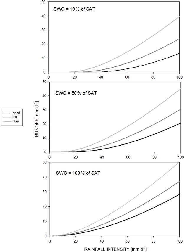
2160                  D. Hidy et al.: Soil-related developments of the Biome-BGCMuSo v6.2 terrestrial ecosystem model

   In spite of its popularity and proven applicability, the de-        The water balance module of Biome-BGCMuSo has five
velopment of Biome-BGC was temporarily stopped (the lat-            major components to describe soil-water-related processes at
est official NTSG version is Biome-BGC 4.2; https://www.            daily resolution (listed here following the order of calcula-
ntsg.umt.edu, last access: November 2021). One major draw-          tion): pond water accumulation and runoff, infiltration and
back of the model was its relatively poor performance in            downward gravitational flow (percolation), water movement
modeling managed ecosystems and the simplistic soil water           within the soil (diffusion) driven by water potential gradi-
balance submodel using a single soil layer only.                    ent, evaporation and transpiration (root water uptake), and
   Our team started to develop the Biome-BGC model further          the downward and upward fluxes to and from groundwater.
in 2006. According to the logic of the team, the new model          In the following subsections these five major components are
branch was planned to be the continuation of the Biome-             described.
BGC model with regard to the original concept of the devel-
opers (keeping the model code open-source, providing de-            3.1   Pond water accumulation and runoff
tailed documentation, and providing support for users).
   The starting point of our model development was Biome-           Precipitation can reach the surface as rain or snow (below
BGC v4.1.1 that was a result of the model improvement ac-           0 ◦ C snow accumulation is assumed). Snow water melts from
tivities of the Max Planck Institute (Vetter et al., 2008). De-     the snowpack as a function of temperature and radiation and
velopment of the Biome-BGCMuSo model branch has a long              is added to the precipitation input.
history by now. Previous model developments were docu-                 The canopy can intercept rain. The intercepted volume
mented in Hidy et al. (2012, 2016). Below, we provide a de-         goes into the canopy water pool, which can evaporate. No
tailed description of the new developments that are included        canopy interception of snow is assumed. The throughfall
in Biome-BGCMuSo v6.2, which is the latest version re-              (complemented with the amount of melted snow) gives the
leased in September 2021. A comprehensive review of the             potential infiltration.
input data requirement of the model, together with an ex-              A new development in Biome-BGCMuSo v6.2 is that
planation of the input data structure, is available in the user     maximum infiltration is calculated based on the saturated hy-
guide (Hidy et al., 2021). In this paper we refer to some in-       draulic conductivity and the SWC of the topsoil layers. If
put files (e.g., soil file, plant file) that are described in the   the potential infiltration exceeds the maximum infiltration,
user guide in detail.                                               pond water can be formed. If the sum of the precipitation
   One of the most important novelties and advantages of            and the actual pond height minus the maximum infiltration
the new model version (Biome-BGCMuSo v6.2) compared                 rate is greater than the maximum pond height, the excess wa-
to any previous versions due to the extensive and detailed          ter is added to surface runoff detailed below (Balsamo et al.,
soil parameter set (the current version has 79, MuSo 4.0 has        2009). The maximum pond height is an input parameter. Wa-
39, and the original model version has only 6 adjustable soil-      ter from the pond can infiltrate into the soil at a rate at which
related parameters) is that the parameterization of the model       the topsoil layer can absorb it. Evaporation of pond water is
is much more flexible. But it might, of course, be a challeng-      assumed to be equal to the potential evaporation.
ing task to define all of the input parameters. In order to sup-       Surface runoff is the water flow occurring on the surface
port practical application of the model, the user guide con-        when a portion of the precipitation cannot infiltrate into the
tains proposed values for most of the new parameters (Hidy          soil. Two types of surface runoff processes can be distin-
et al., 2021).                                                      guished: Hortonian and Dunne. Hortonian runoff is unsatu-
                                                                    rated overland flow that occurs when the rate of precipitation
                                                                    exceeds the rate at which water can infiltrate. The other type
                                                                    of surface runoff is the Dunne runoff (also known as the sat-
3   Soil-hydrology-related developments                             uration overland flow), which occurs when the entire soil is
                                                                    saturated but the rain continues to fall. In this case the rain-
In Biome-BGCMuSo v6.2 a 10-layer soil submodel was im-              fall immediately triggers pond water formation and (above
plemented. Previous model versions included a seven-layer           the maximum pond water height) surface runoff. The han-
submodel, which turned out to be insufficient to capture hy-        dling of these processes is presented in the soil hydrological
drological events like drying of the topsoil layers with suf-       module of Biome-BGCMuSo v6.2.
ficient accuracy. The thicknesses of the layers from the sur-          Calculation of Hortonian runoff (kg H2 O m−2 d−1 ) is
face to the bottom are 3, 7, 20, 30, 30, 30, 30, 50, 200, and       based on a semi-empirical method and uses the precipitation
600 cm. The center of the given layer represents the depth of       amount (cm d−1 ), the unitless runoff curve number (RCN),
each soil layer. Soil texture can be defined by the percent-        and the actual moisture content status of the topsoil (Rawls
age of sand and silt for each layer separately along with the       et al., 1980; this method is known as the SCS runoff curve
most important physical and chemical parameters (pH, bulk           number method; SCS: soil conservation service). This type
density, characteristic SWC values, drainage coefficient, hy-       of runoff simulation can be turned off by setting RCN to zero.
draulic conductivity) in the soil input file (Hidy et al., 2021).   A detailed description can be found in Sect. S1 in the Sup-

Geosci. Model Dev., 15, 2157–2181, 2022                                              https://doi.org/10.5194/gmd-15-2157-2022
D. Hidy et al.: Soil-related developments of the Biome-BGCMuSo v6.2 terrestrial ecosystem model                                   2161

                                                                       hydraulic conductivity, cm d−1 ; the user can set its value or
                                                                       the model based on soil texture estimates it internally; see
                                                                       Hidy et al., 2016). A detailed description of the method can
                                                                       be found in Sect. S2 in the Supplement. Drainage from the
                                                                       bottom layer is a net loss for the soil profile.
                                                                          Water diffusion that is the capillary water flow between
                                                                       the soil layers is calculated to account for the relatively slow
                                                                       movement of water. The flow rate is a function of the water
                                                                       content difference of two adjacent layers and the soil water
                                                                       diffusivity at the boundary of the layers, which is determined
                                                                       based on the average water content of the two layers. A de-
                                                                       tailed mathematical description of the method can be found
                                                                       in Sect. S3 in the Supplement.
                                                                          A detailed description of the Richards method can be
                                                                       found in Hidy et al. (2012). To support efficient and robust
                                                                       calculations of soil water fluxes a dynamically changing time
                                                                       step was introduced in version 4.0 (Hidy et al., 2016). The
                                                                       implementation of the more sophisticated Richards method
                                                                       is still in an experimental phase requiring rigorous testing
                                                                       and validation in the future.

                                                                       3.3     Evapotranspiration

                                                                       Biome-BGCMuSo, like its predecessor Biome-BGC, esti-
                                                                       mates evaporation of leaf-intercepted water, bare soil evapo-
                                                                       ration, and transpiration to estimate the total evapotranspira-
                                                                       tion at a daily level. The potential rates of all three processes
Figure 1. Hortonian runoff as a function of rainfall intensity, soil   are calculated based on the Penman–Monteith (PM) method.
type, and actual soil water content of the topsoil layer. Sand soil    PM equation requires net radiation (minus soil heat flux) and
means 92 % sand, 4 % silt, and 4 % clay; silt soil means 8 % sand,     conductance values by definition using different parameteri-
86 % silt, and 6 % clay; clay soil means 20 % sand, 20 % silt, and     zation for the different processes. The model calculates leaf-
60 % clay. SWC and SAT denote soil water content and saturation,       and canopy-level conductances of water vapor and sensible
respectively.                                                          heat fluxes to be used in Penman–Monteith calculations of
                                                                       canopy evaporation and canopy transpiration. Note that in the
                                                                       Biome-BGC model family the direct wind effect is ignored
plement. The amount of runoff as a function of the soil type           but can be considered indirectly by adjusting boundary layer
and the actual SWC is presented in Fig. 1.                             conductance to site-specific conditions. A possible future di-
                                                                       rection might be the extension of the model logic to consider
3.2   Infiltration, percolation, and diffusion                         the wind effect directly.
There are two optional methods in Biome-BGCMuSo v6.2
to calculate soil water movement between soil layers and ac-           3.3.1    Canopy evaporation
tual SWC layer by layer. The first one is a cascade method
(also known as tipping bucket method), and the second is a             If there is intercepted water, this portion of evaporation is
physical method based on the Richards equation. The tipping            calculated using the canopy resistance (reciprocal of conduc-
bucket method has a long history in crop modeling and is               tance) to evaporated water and the resistance to sensible heat.
considered to be a successful, well-evaluated algorithm that           The time required for the water to evaporate based on the av-
can accurately simulate downward water flow in the soil.               erage daily conditions is calculated and subtracted from the
   The cascade method uses a semi-empirical input param-               day length to get the effective day length for evapotranspi-
eter (DC: drainage coefficient, d−1 ) to calculate the down-           ration. Combined resistance to convective and radiative heat
ward water flow rate. When the SWC of a soil layer exceeds             transfer is calculated based on canopy conductance of va-
field capacity (FC), a fraction (equal to DC) of the water             por and leaf conductance of sensible heat, both of which are
amount above FC goes to the layer next below. If DC is not             assumed to be equal to the boundary layer conductance. Be-
set in the soil input file, it is estimated from the saturated hy-     sides the conductance and resistance parameters the canopy-
                                            0.339
draulic conductivity: DC = 0.1122 · KSAT          (KSAT : saturated    absorbed shortwave radiation drives the calculation. Note

https://doi.org/10.5194/gmd-15-2157-2022                                                 Geosci. Model Dev., 15, 2157–2181, 2022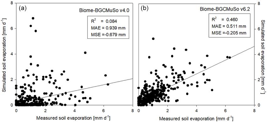
2162                     D. Hidy et al.: Soil-related developments of the Biome-BGCMuSo v6.2 terrestrial ecosystem model

that the canopy evaporation routine was not modified signif-
icantly in Biome-BGCMuSo.

3.3.2   Soil evaporation

In order to estimate soil evaporation, first the potential evap-
oration is calculated, assuming that the resistance to vapor is
equal to the resistance to sensible heat and assuming no addi-
tional resistance component. Both resistances are assumed to
be equal to the actual aerodynamic resistance. Actual aero-
dynamic resistance is a function of the actual air pressure
and air temperature as well as the potential aerodynamic re-
sistance (potRair in s m−1 ). potRair was a fixed value in the
previous model versions (107 s m−1 ). Its value was derived
from observations over bare soil in tiger bush in southwest-
ern Niger (Wallace and Holwill, 1997). In Biome-BGCMuSo
v6.2, the potRair is an input parameter that can be adjusted
by the user (Hidy et al., 2021). Another new development in
Biome-BGCMuSo v6.2 is the introduction of an upper limit
for daily potential evaporation (evaplimit ) that is determined
by the available energy (incident shortwave flux that reaches
the soil surface):
              irad · dayl
evaplimit =               ,                                 (1)
                LHvap

where irad is the incident shortwave flux density (W m−2 ),
dayl is the length of the day in seconds, and LHvap is the la-
tent heat of vaporization (the amount of energy that must be
                                                                   Figure 2. Surface coverage as a function of the amount of surface
added to liquid to transform into gas; J kg−1 ). This feature      residue or mulch (a) and the evaporation reduction factor (evap-
was missing from previous model versions, resulting in con-        REDmulch) as a function of mulch coverage (b) using different
siderable overestimation of evaporation on certain days that       mulch-specific soil parameters (pREDmulch). See text for details.
was caused by the missing energy limitation on evaporation.
   A new feature in Biome-BGCMuSo v6.2 is the calculation
of the actual evaporation from the potential evaporation and       mulch (mu, kg C m−2 ) with parameters p1mulch , p2mulch , and
the square root of time elapsed since the last precipitation       p3mulch (soil parameters) based on the method of Rawls et al.
(expressed by days; Ritchie, 1998). This is another method         (1980).
that has been used by the crop modeler community for many
years. A detailed description of the algorithm can be found        mulchCOV = p1mulch · (mu/p2mulch )p3mulch                    (2)
in Sect. S4 in the Supplement.                                                                      mulchCOV
                                                                   evapREdmulch = pREDmulch            100                      (3)
   One major new development in Biome-BGCMuSo v6.2 is
the simulation of the reducing effect of surface residue or        Another simulated effect of surface residue cover is the ho-
mulch cover on bare soil evaporation. Here we use the term         mogenization of soil temperature between 0 and 30 cm depth
“mulch” to quantify surface residue cover in general, keep-        (layers 1, 2, and 3). The functional forms of surface coverage
ing in mind that mulch is typically a human-induced cover-         and the evaporation reduction factor are presented in Fig. 2.
age. Surface residue includes aboveground litter and coarse
woody debris as well.                                              3.3.3   Transpiration
   The evaporation reduction effect (evapREDmulch; unit-
less) is a variable between 0 and 1 (0 means full limitation,      In order to simulate transpiration, first transpiration demand
and 1 means no limitation) estimated based on a power func-        (TD, kg H2 O m−2 d−1 ) is calculated using the Penman–
tion of the surface coverage (mulchCOV in %) and a soil-           Monteith equation separately for sunlit and shaded leaves.
specific constant set by the user (pREDmulch; see Hidy et          TD is a function of leaf-scale conductance to water vapor,
al., 2021). If variable mulchCOV reaches 100 % it means that       which is derived from stomatal, cuticular, and leaf boundary
the surface is completely covered. If mulchCOV is greater          layer conductances. A novelty in Biome-BGCMuSo v6.2 is
than 100 % it means the surface is covered by more than one        that potential evapotranspiration is also calculated using the
layer. Surface coverage is a power function of the amount of       maximal stomatal conductance instead of the actual stomatal

Geosci. Model Dev., 15, 2157–2181, 2022                                             https://doi.org/10.5194/gmd-15-2157-2022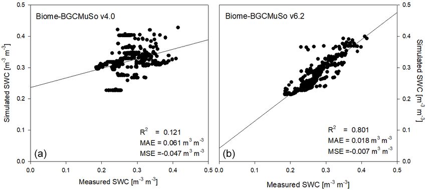
D. Hidy et al.: Soil-related developments of the Biome-BGCMuSo v6.2 terrestrial ecosystem model                              2163

conductance, which means that stomatal aperture is not af-         the limitation of stomatal conductance and decomposition. A
fected by the soil moisture status (in contrast to the actual      practical advantage of using SWC as a factor in the stress
one).                                                              function is that it is easier to measure in the field and the
   TD is distributed across the soil layers according to the       changes in the driving function are much smoother than in
actual root distribution using an improved method (the logic       the case of 9. The disadvantage is that SWC is not compa-
was changed since Biome-BGCMuSo v4.0). From the plant-             rable among different soil types (in contrast to 9).
specific root parameters and the actual root weight Biome-            The maximum of SWC is the saturation value; the mini-
BGCMuSo calculates the number of layers in which roots             mum is the wilting point or the hygroscopic water depend-
can be found together with the root mass distribution across       ing on the type of simulated process. The novelty of Biome-
the layers (Jarvis, 1989; Hidy et al., 2016). If there is not      BGCMuSo v6.2 is that the hygroscopic water, the wilting
enough water in a given soil layer to fulfill the transpiration    point, the field capacity, and the saturation values are calcu-
demand, the transpiration flux from that layer is limited, and     lated internally by the model based on the soil texture data,
below the wilting point (WP) it is set to zero. The sum of         or they can be defined in the input file layer by layer.
layer-specific transpiration fluxes across the root zone gives        In Biome-BGCMuSo v6.2 the so-called soil moisture
the actual transpiration flux. A detailed description of the al-   stress index (SMSI) is calculated to represent overall soil
gorithm can be found in Sect. S5 in the Supplement.                stress conditions. SMSI is affected by the length of the
                                                                   drought event (SMSE: extent of soil stress) and the sever-
3.4   Effect of groundwater                                        ity of the drought event (SMSL: length of soil stress), and
                                                                   it is aggravated by extreme temperature (extremT: effect of
Simulation of the groundwater effect was introduced in             extreme heat). SMSI is equal to zero if no soil moisture lim-
Biome-BGCMuSo v4.0 (Hidy et al., 2016), but the method             itation occurs and equal to 1 in the case of full soil mois-
has been significantly improved, and the new algorithm it          ture limitation. SMSI is used by the model for plant senes-
is now available in Biome-BGCMuSo v6.2. In the recent              cence calculations (presentation of plant-related processes is
model version there is an option to provide an additional in-      the subject of a forthcoming publication). The components
put file with the daily values of the groundwater table depth      of SMSI are explained in detail below.
(GWdepth in meters).
   Groundwater may affect soil hydrological and plant phys-        SMSI = 1 − SMSE · SMSL · extremT                            (4)
iological processes if the water table is closer to the root
zone than the thickness of the capillary fringe (that is the
region saturated from groundwater via the capillary effect).          The magnitude of soil moisture stress (SMSE) is calcu-
The thickness of the capillary fringe (CF in meters) is es-        lated layer by layer based on SWC. Regarding soil moisture
timated using literature data and depends on the soil type         stress two different processes are distinguished: drought (i.e.,
(Johnson and Ettinger model; Tillman and Weaver, 2006).            low SWC close to or below WP) and anoxic conditions (i.e.,
Groundwater table distance (GWdist in m) for a given layer         after large precipitation events or in the presence of a high
is defined as the difference between GWdepth and the depth         groundwater table; Bond-Lamberty et al., 2007). An impor-
of the midpoint of the layer.                                      tant novelty of Biome-BGCMuSo v6.2 is the soil curvature
   The layers completely below the groundwater table are as-       parameter (q), which is introduced to provide a mechanism
sumed to be fully saturated. In the case of layers within the      for soil-texture-dependent drought stress as it can affect the
capillary fringe (GWdist < CF), the calculation of water bal-      shape of the soil stress function (which means a possibility
ance changes: the FC rises, and thus the difference between        for a nonlinear ramp function):
saturation (SAT) and FC decreases, and the layer charges
gradually until the increased FC value is reached. The FC ris-     SMSEi = 0;
ing effect of groundwater for the layers above the water table
is calculated based on the ratio of the groundwater distance              SWCi < SWCiWP
                                                                                                          !q
and the capillary fringe thickness, but only after the water                      SWCi − SWCiWP
contents of the layers below have reached their modified FC        SMSEi =                                     ;
                                                                                SWCidrought − SWCiWP
values. A detailed description of the groundwater effect can
be found in Sect. S6 in the Supplement.                                   SWCiWP ≤ SWC < SWCidrought
                                                                   SMSEi = 1;
3.5   Soil moisture stress
                                                                          SWCidrought ≤ SWC ≤ SWCianoxic
In the original Biome-BGC model the effect of changing soil                     SWCiSAT − SWCi
water content on photosynthesis and decomposition of soil          SMSEi =                            ;
organic matter is expressed in terms of soil water potential                  SWCiSAT − SWCianoxic
(9). Instead of 9, the SWC is also widely used to calculate               SWCi > SWCianoxic                                    (5)

https://doi.org/10.5194/gmd-15-2157-2022                                             Geosci. Model Dev., 15, 2157–2181, 2022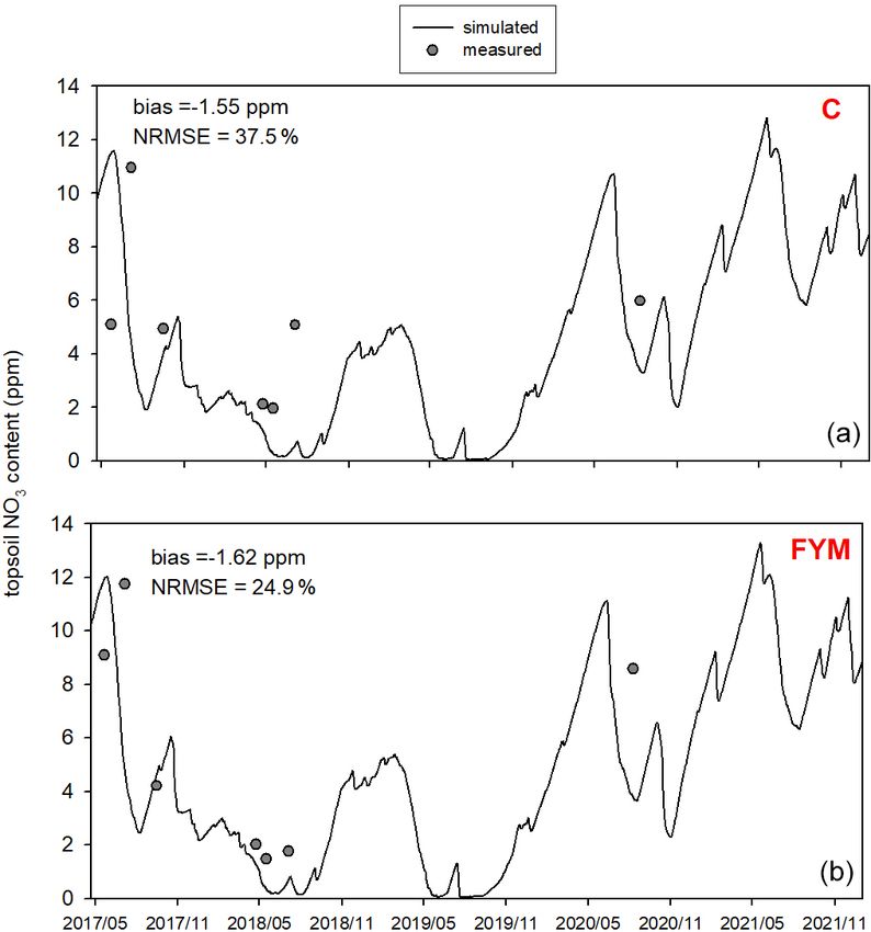
2164                     D. Hidy et al.: Soil-related developments of the Biome-BGCMuSo v6.2 terrestrial ecosystem model

where q is the curvature of the soil stress function, and             Instead of defining a single litter, soil organic carbon
SWCidrought and SWCianoxic are critical SWC values for cal-        (SOC), and nitrogen pool, we implemented separate carbon
culating soil stress.                                              and nitrogen pools for each soil layer in the form of soil
   In order to make the SWC values comparable between dif-         organic matter (SOM) and litter in Biome-BGCMuSo v6.2.
ferent soil types, SWCidrought and SWCianoxic can be set in        The changes in the mass of the carbon and nitrogen pools
normalized form (such as in Eq. 4) as part of the ecophysio-       are calculated layer by layer. Mortality fluxes (whole plant
logical parameterization of the model. More details about the      mortality, senescence, litterfall) of aboveground plant mate-
adjustment of the critical SWC values can be found in Hidy         rial are transferred into the litter pools of the topsoil layers
et al. (2021).                                                     (0–10 cm, layers 1–2). Mortality fluxes of belowground plant
   The layer-specific soil moisture stress extent values are       material are transferred into the corresponding soil layers
summed across the root zone using the relative quantity of         based on their location within the root zone. Due to plough-
roots in the layers (RPi ) as weighting factors to obtain the      ing and leaching, carbon and nitrogen can also be relocated to
overall soil moisture stress extent (SMSE):                        deeper layers. The plant material turning into the litter com-
           i=nr                                                    partment is divided between the different types of litter pools
                                                                   (labile, unshielded cellulose, shielded cellulose, and lignin)
           X
SMSE =            SMSEi · RPi ,                             (6)
           i=0                                                     according to the parameterization. Litter and soil decompo-
            zi               i
                                                                   sition fluxes (carbon and nitrogen fluxes from litter to soil
RPi = RD        · e−RD·(mid /RL) ,                           (7)   pools) are calculated layer by layer, depending on the actual
            RL
                                                                   temperature and SWC of the corresponding layers. Vertical
where nr is the number of soil layers in which roots can           mixing of soil organic matter between the soil layers (e.g.,
be found, RL is the actual length of roots, and RD is the          bioturbation) is not implemented in the current model ver-
rooting distribution parameter (ecophysiological parameter;        sion.
see details in the user guide; Hidy et al., 2021). In the cur-        Figure 3 shows the most important simulated soil and lit-
rent model version SMSE can also affect the entire photo-          ter processes. N fixation (Nf) is the N input from the atmo-
synthetic machinery by the introduction of an empirical pa-        sphere to soil layers in the root zone by microorganisms. The
rameter. This mechanism is responsible for accounting for          user can set its annual value as an input parameter. N depo-
the non-stomatal effect of drought on photosynthesis (de-          sition (Nd) is the N input from the atmosphere to the top-
tails about this algorithm will be published in a separate pa-     soil layers (see below). The user can set its annual value as
per). Since there is no mechanistic representation behind this     a site-specific parameter in the initialization input file. Nitro-
empirical downregulation of photosynthesis, further tests are      gen deposition can be provided by annually varying values
needed for the correct setting of this parameter preferentially    as well. Plant uptake (PU) is the absorption of mineral N by
using eddy covariance data.                                        plants from the soil layers in the root zone. Mineralization
   The factor (SMSL) related to soil moisture stress length is     (MI) is the release of plant-available nitrogen (flux from soil
the ratio of the critical soil moisture stress length (ecophys-    organic matter to mineralized nitrogen). Immobilization (IM)
iological parameter) and the sum of the daily (1 − SMSE)           is the consumption of inorganic nitrogen by microorganisms
values. This cumulated value restarts if SMSE is equal to 1        (flux from mineralized nitrogen to soil organic matter). Ni-
(no stress). Extreme heat (extremT) is also considered and is      trification (NI) is the biological oxidation of ammonium to
taken into account in the final stress function (see above) by     nitrate through nitrifying bacteria. Denitrification (DN) is a
using a ramp function. Its parameterization thus requires the      microbial process whereby nitrate (NO3 − ) is reduced and
setting of two critical temperature limits that define the ramp    converted to nitrogen gas (N2 ) through intermediate nitrogen
function (set by the ecophysiological parameterization; see        oxide gases. Leaching (L) is the loss of water-soluble min-
Hidy et al., 2021). Its characteristic temperature values can      eral nitrogen from the soil layers. If leaching occurs in the
be set by parameterization (ecophysiological input file).          lowermost soil layer that means loss of N from the simulated
                                                                   system. Litterfall (LI) is the plant material transfer from plant
4     Soil carbon and nitrogen cycles                              compartments to litter. Decomposition is the C and N transfer
                                                                   from litter to soil pools and between soil pools. In the case
4.1    Soil–litter module                                          of woody vegetation coarse woody debris (CWD) contains
                                                                   the woody plant material after litterfall before physical frag-
We made substantial changes in the soil biogeochemistry            mentation. Litter has also four sub-pools based on composi-
module of the Biome-BGC model. Previous model versions             tion: labile (L1), unshielded and shielded cellulose (L2, L3),
already offered solutions for multilayer simulations (Hidy et      and lignin (L4). Soil organic matter also has four sub-pools
al., 2012, 2016), but some pools still inherited the single-       based on turnover rate: labile (S1), medium (S2), slow (S3),
layer logic of the original model. In the new model version        and passive (recalcitrant; S4). The soil-mineralized nitrogen
all relevant soil processes are separated layer by layer, which    pool contains the inorganic N forms of the soil: ammonium
is a major step forward.                                           and nitrate.

Geosci. Model Dev., 15, 2157–2181, 2022                                             https://doi.org/10.5194/gmd-15-2157-2022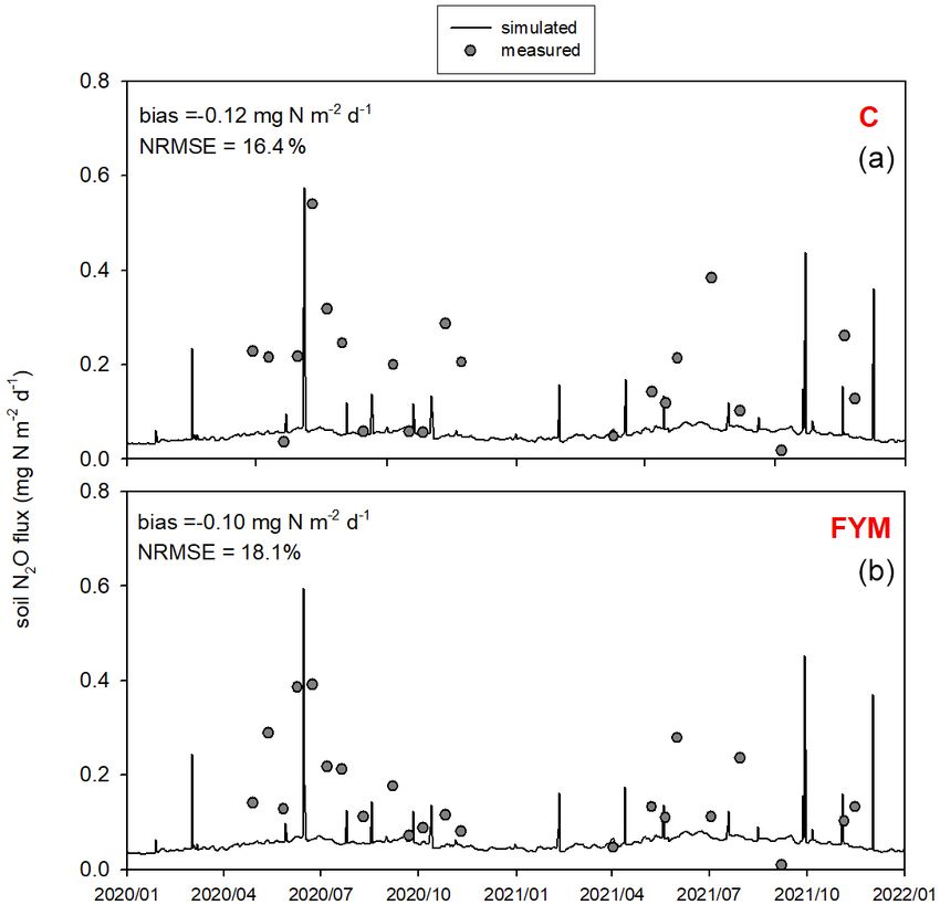
D. Hidy et al.: Soil-related developments of the Biome-BGCMuSo v6.2 terrestrial ecosystem model                                         2165

Figure 3. Soil- and litter-related simulated carbon and nitrogen fluxes (arrows) as well as pools (rectangles) in Biome-BGCMuSo v6.2. HR:
heterotrophic respiration, IM: immobilization, MI: mineralization, PU: plant uptake, LI: litterfall, NI: nitrification, D: decomposition (DL :
decomposition of litter, DS : decomposition of SOM, DC : fragmentation of coarse woody debris), L: leaching, Nf: nitrogen fixation, Nd:
nitrogen deposition, DN: denitrification. L represents loss of C and N from the simulated system.

4.2   Decomposition                                                         For the calculation of nitrogen mineralization, first respi-
                                                                         ration cost (respiration fraction) is estimated. Mineralization
                                                                         is then a function of the remaining part of the pool and its
In the decomposition module (i.e., converging cascade
                                                                         C : N ratio. The nitrogen mineralization fluxes of the SOM
scheme; Thornton, 1998) the fluxes between litter and soil
                                                                         pools are functions of the potential rate constant (reciprocal
pools are calculated layer by layer. The potential fluxes are
                                                                         of residence time) and the integrated response function that
modified in the case of N limitation when the potential gross
                                                                         accounts for the impact of multiple environmental factors.
immobilization is greater than the potential gross mineraliza-
                                                                         The integrated response function of decomposition is a prod-
tion.
                                                                         uct of the response functions of depth, soil temperature, and
   To explain the decomposition processes implemented in
                                                                         SWC (Fr (d)D , Fr (T )D , Fr (SWC)D ; Fig. 5). Its detailed de-
Biome-BGCMuSo v6.2 the main carbon and nitrogen pools
                                                                         scription can be found in Sect. S7. The dependence of the
as well as fluxes between litter and soil organic and inorganic
                                                                         three different factors on depth, temperature, and SWC with
(mineralized) matter are presented in Fig. 4.
                                                                         default parameters is presented in Fig. 5.
   In the original Biome-BGC and in previous Biome-
BGCMuSo versions the C : N ratio (CN) of the soil pools was
fixed in the model code. One of the new features in Biome-               4.3    Soil nitrogen processes
BGCMuSo v6.2 is that the CN of the passive soil pool (S4
in Fig. 4; recalcitrant soil organic matter) can be set by the           In Biome-BGCMuSo v6.2 separate ammonium (sNH4) and
user as a soil parameter. The CN of the other soil pools (la-            nitrate (sNO3) soil pools are implemented instead of a gen-
bile, medium, and slow; S1, S2, and S3) is calculated based              eral mineralized nitrogen pool. This was a necessary step for
on the proportion of fixed CN values of the original Biome-              the realistic representation of many internal processes like
BGC (CNlabile /CNpassive = 1.2, CNmedium /CNpassive = 1.2,               plant nitrogen uptake, nitrification, denitrification, consider-
CNslow /CNpassive = 1). Note that the CN of the donor and                ation of the effect of different mineral and organic fertilizers,
acceptor pools is used in decomposition calculations (see de-            and N2 O emission.
tails in Sect. S7 in the Supplement), and as a result these pa-             It is important to introduce the availability concept that
rameters set the C : N ratio of the soil pools. The donor and            Biome-BGCMuSo uses and is associated with the ammo-
acceptor pools can be seen in Figs. 3 and 4.                             nium and nitrate pools. We use the logic proposed by Thomas

https://doi.org/10.5194/gmd-15-2157-2022                                                     Geosci. Model Dev., 15, 2157–2181, 2022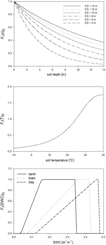
2166                    D. Hidy et al.: Soil-related developments of the Biome-BGCMuSo v6.2 terrestrial ecosystem model

Figure 4. Overview of the converging cascade model of litter and soil organic matter decomposition that is implemented in Biome-BGCMuSo
v6.2. The notation rf represents the respiration fraction of the different transformation fluxes, and τ is the residence time (reciprocal of the
rate constants, which is the turnover rate). IM/MI: immobilization and mineralization fluxes, HR: heterotrophic respiration. Note that both
the respiration fraction and the turnover rate parameters can be adjusted through parameterization.

et al. (2013), which means that the plant has access only to              (i − 1), respectively; PUisNH4 and PUisNO3 are the plant up-
a part of the given inorganic nitrogen pool. The unavailable              take fluxes of ammonium and nitrate, respectively; IMisNH4
part is buffered as it is associated with soil aggregates and             and IMisNO3 are the immobilization fluxes of ammonium and
is unavailable for plant uptake. The available part of ammo-              nitrate, respectively; MIisNH4 and MIisNO3 are the mineraliza-
nium is calculated based on the NH4 mobile proportion (that               tion fluxes of ammonium and nitrate, respectively; NIisNH4 is
is a soil parameter set to 10 % according to Thomas et al.,               the nitrification flux of ammonium; and DNisNO3 is the deni-
2013; Hidy et al., 2021) and the actual pool. The available               trification flux of nitrate.
part of nitrate is assumed to be 100 %.                                      In the following subsections the different terms of the
   The amount of ammonium and nitrate is determined                       equations are described in detail.
layer by layer controlled by input and output fluxes (F ,
kg N m−2 d−1 ) listed below:                                              Input to the sNH4 and sNO3 pools (IN in Eqs. 6 and 7)
 i
FsNH4 = INisNH4 − LisNH4 + Li−1      i        i
                            sNH4 − PUsNH4 − IMsNH4                        According to the model logic N fixation occurs in the root
        + MIisNH4 − NIisNH4 ,                                    (8)      zone layers. Its distribution between sNH4 and sNO3 pools
                                                                          is calculated based on their actual available proportion in the
 i
FsNO3 = INisNO3 − LisNO3 + Li−1        i        i
                              sNO3 − PUsNO3 − IMsNO3                      actual layer (NH4propi ):
        + MIisNO3 − DNisNO3 ,                                    (9)      NH4propi = sNH4availi + sNO3availi ,                             (10)
where  INisNH4and    INisNO3
                          are the input fluxes to the ammo-                                   i                   i
                                                                          where sNH4avail and sNO3avail are the available part of
nium and nitrate pools, respectively; LisNH4 , Li−1     i
                                                sNH4 , LsNO3 ,            the sNH4 and sNO3 pools in the actual layer.
     i−1
and LsNO3 represent the amount of leached mineralized am-                   N-deposition-related nitrogen input is associated with the
monium and nitrate from a layer (i) or from the upper layer               0–10 cm soil layers assuming uniform distribution across

Geosci. Model Dev., 15, 2157–2181, 2022                                                      https://doi.org/10.5194/gmd-15-2157-2022
D. Hidy et al.: Soil-related developments of the Biome-BGCMuSo v6.2 terrestrial ecosystem model 2167
layers 1–2 in the model, and the distribution between sNH4
and sNO3 pools is calculated based on the proportion of the
NH4 flux of the N deposition soil parameter (Hidy et al.,
2021).
Organic and inorganic fertilization is also an optional ni-
trogen input. The amount and composition (NH4 + and NO3 −
content) can be set in the fertilization input file.
Leaching – downward movement of mineralized N (L in
Eqs. 6 and 7)
The amount of leached mineralized N (mobile part of the
given N pool) from a layer is directly proportional to the
amount of drainage and the available part of the sNH4 and
sNO3 pools. Leaching from the layer above is a net gain,
while leaching from actual layer is a net loss for the actual
layer. Leaching is described in Sect. 4.5.
Plant uptake by roots (PU in Eqs. 6 and 7)
N uptake required for plant growth is estimated in the pho-
tosynthesis calculations, and the amount is distributed across
the layers in the root zone. The partition of the N uptake be-
tween sNH4 and sNO3 pools is calculated based on their ac-
tual available proportion in each layer.
Mineralization and immobilization (MI and IM Eqs. 6
and 7)
Mineralization and immobilization calculations are detailed
in Sect. 4.2. The distribution of these N fluxes between sNH4
and sNO3 pools is calculated based on their actual available
proportion in each layer.
Nitrification (NI Eqs. 6 and 7)
Nitrification is a function of the soil ammonium content, the
net mineralization, and the response functions of tempera-
ture, soil pH, and SWC (Fr (pH)NI , Fr (T )NI , and Fr (SWC)NI ,
respectively) based on the method of Parton et al. (2001) and
Thomas et al. (2013). Its detailed mathematical description
can be found in Sect. S8 in the Supplement. The response
functions with proposed parameters are shown in Fig. 6.
Denitrification (DN Eqs. 6 and 7)
Denitrification flux is estimated with a simple formula
(Thomas et al., 2013):
Figure 5. The dependence of the individual factors that form the
complex environmental response function of decomposition on DNi = DNcoeff · SOMrespi · sNO3availi · WFPSi , (11)
depth (Fr (d)D ), temperature (Fr (T )D ), and SWC in the case of dif-
ferent soil types (Fr (SWC)D ). ED is the e-folding depth, which is where DN of the actual layer is the product of the
one of the adjustable soil parameters of the model. For the definition available nitrate content (sNO3avail, kg N m−2 ), SOMrespi
of sand, silt, and clay see Fig. 1. (g C m−2 d−1 ) is the SOM-decomposition-related respiration
cost, WFPSi is the water-filled pore space, and DNcoeff is
the soil-respiration-related denitrification rate (g C−1 ), which
is an input soil parameter (Hidy et al., 2021). The unitless
https://doi.org/10.5194/gmd-15-2157-2022 Geosci. Model Dev., 15, 2157–2181, 20222168 D. Hidy et al.: Soil-related developments of the Biome-BGCMuSo v6.2 terrestrial ecosystem model
4.4 N2 O emission and N emission
During both nitrification and denitrification N2 O emission
occurs, which (added to the N2 O flux originating from graz-
ing processes if applicable) contributes to the total N2 O emis-
sion of the examined ecosystem.
In Biome-BGCMuSo v6.2 a fixed part (set by the coeffi-
cient of the N2 O emission of the nitrification input soil pa-
rameter; Hidy et al., 2021) of nitrification flux is lost as N2 O
and not converted to NO3 .
During denitrification, nitrate is transformed into N2 and
N2 O gas depending on the environmental conditions: NO3
availability, total soil respiration (proxy for microbial activ-
ity), SWC and pH. The denitrification-related N2 /N2 O ra-
tio input soil parameter is used to represent the effect of the
soil type on the N2 /N2 O ratio (del Grosso et al., 2000; Hidy
et al., 2021). Detailed mathematical description of the algo-
rithm can be found in Sect. S9 in the Supplement.
4.5 Leaching of dissolved matter
Leaching of nitrate, ammonium, and dissolved organic car-
bon and nitrogen (DOC and DON) content from the actual
layer is calculated as the product of the concentration of the
dissolved component in the soil water and the amount of wa-
ter (drainage plus diffusion) leaving the given layer either
downward or upward. The dissolved component (concentra-
tion) of organic carbon is calculated from the SOC pool con-
tents and the corresponding fraction of the dissolved part of
SOC soil parameters. The dissolved component of the or-
ganic nitrogen content of the given soil pool is calculated
from the carbon content and the corresponding C : N ratio.
The downward leaching is net loss from the actual layer and
net gain for the next layer below; the upward flux is net loss
for the actual layer and net gain for the next layer up. The
downward leaching of the bottom active layer (ninth) is net
loss for the system. The upward movement of dissolved sub-
stance from the passive (10th) layer is net gain for the system.
5 Case studies
Figure 6. The dependence of the individual factors of the environ-
mental response function of nitrification on soil pH (Fr (pH)NI ), 5.1 Evaluation of soil hydrological simulation
temperature (Fr (T )NI ), and SWC Fr (SWC)NI in the case of dif-
ferent soil types. The pH and temperature response functions are In order to evaluate the functioning of the new model ver-
independent of the soil texture. sion (and to compare simulation results made by the current
and previously published model version), a case study is pre-
sented regarding soil water content and soil evaporation sim-
ulations. The results of a bare soil simulation (i.e., no plant
is assumed to be present) are compared to observation data
from a weighing lysimeter station installed at Martonvásár,
Hungary (47◦ 180 57.600 N, 18◦ 470 25.600 E), in 2017. The cli-
water-filled pore space is the ratio of the actual and saturated mate of the area is continental with a 30-year average tem-
SWC. SOM-decomposition-associated respiration is the sum perature of 11.0 ◦ C (−1 ◦ C in January and 21.2 ◦ C in July)
of the heterotrophic respiration fluxes of the four soil com- and annual rainfall of 548 mm based on data from the on-site
partments (S1–S4, Fig. 4). weather station.
Geosci. Model Dev., 15, 2157–2181, 2022 https://doi.org/10.5194/gmd-15-2157-2022D. Hidy et al.: Soil-related developments of the Biome-BGCMuSo v6.2 terrestrial ecosystem model 2169
The station consists of 12 scientific lysimeter columns 2 m In Fig. 10 the comparison of the simulated and observed
deep with 1 m diameter (Meter Group Inc., USA) and with daily SWC from the lysimeter experiment is presented.
soil temperature, SWC, and soil water potential sensors in- Based on the model evaluation it seems that the simulation
stalled at 5, 10, 30, 50, 70, 100, and 150 cm depth. Observa- with the new model version is much closer to observations
tion data for 2020 from six columns without vegetation cover than with old version (4.0). The results obtained from v4.0
(i.e., bare soil) were used to validate the model. are consistent with earlier findings about the incorrect repre-
Raw lysimeter observation data were processed using stan- sentation of the annual SWC cycle (Hidy et al., 2016; Sándor
dard methods. Bare soil evaporation values were derived et al., 2017).
based on changes in the mass of the soil columns also con- A thorough validation of the improved model based on
sidering the mass change in the drainage water. Additionally, observed SWC and ET datasets from eddy covariance sites
experience has shown that wind speed is related to the high- is planned to be published in an upcoming paper about the
frequency mass change in the soil column mass. To reduce plant-related improvements.
noise, five-point (5 min) moving averages were used based
on Marek et al. (2014). After quality control of the data, the 5.2 Evaluation of the soil nitrogen balance module and
corrected and smoothed lysimeter mass values were used for the simulated soil respiration
the calculations. SWC observations were averaged to daily
resolution to match the time step of the model. Soil-related developments were evaluated with a case study
Observed local meteorology was used to drive the models focusing on topsoil nitrate content, soil N2 O efflux, and soil
for the year 2020. Soil physical model input parameters (field respiration.
capacity, wilting point, bulk density, etc.) were determined in Experimental data were collected in a long-term fertil-
the laboratory using 100 cm3 undisturbed soil samples taken ization experiment that was set up in 1959 at Martonvásár,
from various depths during the installation of the lysimeter Hungary (47◦ 180 4100 N, 18◦ 460 5000 E). According to the FAO-
station. Regarding other soil parameters the proposed values WRB classification system (IUSS Working Group, 2015),
were used. A detailed description of the input soil parameters the soil is a Haplic Chernozem, with 51.4 % sand, 34 %
and their proposed values is presented in the user guide (Hidy silt, and 14.6 % clay content. Bulk density is 1.47 g cm−3 ,
et al., 2021). pH(H2 O) is 7.3, CaCO3 content is 0 %–1 %, and the mean
In Fig. 7 the simulated and observed time series of soil soil organic matter content in the topsoil is 3.2 %. The plant-
evaporation are presented for Martonvásár for 2020. The fig- available macronutrient supply in the soil was poor for phos-
ure shows that the soil evaporation simulation by v6.2 is more phorus and medium to good for potassium based on the Pro-
realistic than by v4.0. Biome-BGCMuSo v4.0 provides very Planta plant nutrition advisory system (Fodor et al., 2011).
low values during summer on some days, which is not in ac- In the long-term fertilization experiment the treatments were
cordance with the observations. Biome-BGCMuSo v6.2 pro- arranged in a random block design with 6 m × 8 m plots in
vides more realistic values during this time period. four replicates. Eight different treatments were set up: con-
In Fig. 8 the simulated and observed SWCs at 10 cm depth trol (zero artificial fertilizer applied), only N, only P, NPK –
are presented with the daily sum of precipitation represent- with farmyard manure, absolute control (zero nutrient sup-
ing the bare soil simulation in Martonvásár for 2020. The soil ply), only N, only P, and NPK – without farmyard manure.
water balance simulation seems to be realistic using v6.2, The crop in the 4-year fertilizer cycles was maize in the first
since the annual course captures the low and high end of and second years and winter wheat in the third and fourth
the observed values. In contrast, Biome-BGCMuSo v4.0 un- years. Here we used data from the absolute control and from
derestimates the range of SWC and provides overestimations the farmyard manure (FYM) treatments only. FYM was ap-
during the growing season (from spring to autumn). With a plied once every 4 years at a rate of 35 t ha−1 in autumn.
couple of exceptions, the simulated values using v6.2 fall into Topsoil nitrate content was measured during 2017, 2018,
the uncertainty range of the measured values defined by the and 2020 on a few occasions by wet chemical reactions us-
standard deviation of the six parallel measurements. This is ing a stream distillation method after KCl extraction of soil
not the case for the simulations with the 4.0 version. samples (Hungarian Standards Institution MSZ 20135:1999;
Model performance was evaluated by quantitative mea- Akhtar et al., 2011).
sures such as the coefficient of determination (R 2 ), mean ab- Dynamic-chamber-based soil N2 O efflux observations
solute error (MAE), and mean signed error (MSE). In Fig. 9 were available from 2020 and 2021. The N2 O efflux mea-
the comparison of the simulated and observed daily evapo- surements with a gas incubation time of 10 min were per-
ration is presented. Based on the performance indicators it formed by using a Picarro G2508 (Picarro, USA) cavity ring-
is obvious that the simulation with the new model version down spectrometer (Christiansen et al., 2015; Zhen et al.,
(v6.2) is much closer to observations than the old version 2021). The cylinder-shaped transparent gas incubation cham-
(v4.0). Biome-BGCMuSo v6.2 slightly underestimated the ber was 16.5 cm in diameter, and its height was 30 cm. N2 O
observations. flux measurements were executed in six replicates per treat-
ment on a biweekly (2020) and precipitation-event-related
https://doi.org/10.5194/gmd-15-2157-2022 Geosci. Model Dev., 15, 2157–2181, 2022You can also read