Global, high-resolution mapping of tropospheric ozone - explainable machine learning and impact of uncertainties - GMD
←
→
Page content transcription
If your browser does not render page correctly, please read the page content below
Model description paper
Geosci. Model Dev., 15, 4331–4354, 2022
https://doi.org/10.5194/gmd-15-4331-2022
© Author(s) 2022. This work is distributed under
the Creative Commons Attribution 4.0 License.

Global, high-resolution mapping of tropospheric ozone –
explainable machine learning and impact of uncertainties
Clara Betancourt1 , Timo T. Stomberg2 , Ann-Kathrin Edrich3,5 , Ankit Patnala1 , Martin G. Schultz1 ,
Ribana Roscher2,4 , Julia Kowalski5 , and Scarlet Stadtler1
1 JülichSupercomputing Centre, Jülich Research Centre, Wilhelm-Johnen-Straße, 52425 Jülich, Germany
2 Institute
          of Geodesy and Geoinformation, University of Bonn, Niebuhrstraße 1a, 53113 Bonn, Germany
3 Aachen Institute for Advanced Study in Computational Engineering Science (AICES), RWTH Aachen University,

Schinkelstrasse 2a, 52062 Aachen, Germany
4 Data Science in Earth Observation, Technical University of Munich, Lise-Meitner-Str. 9, 85521 Ottobrunn, Germany
5 Methods for Model-based Development in Computational Engineering, RWTH Aachen University,

Eilfschornsteinstr. 18, 52062 Aachen, Germany

Correspondence: Scarlet Stadtler (s.stadtler@fz-juelich.de)

Received: 5 January 2022 – Discussion started: 19 January 2022
Revised: 14 April 2022 – Accepted: 11 May 2022 – Published: 3 June 2022

Abstract. Tropospheric ozone is a toxic greenhouse gas with          We provide a rationale for the tools we use to conduct a
a highly variable spatial distribution which is challenging        thorough global analysis. The methods presented here can
to map on a global scale. Here, we present a data-driven           thus be easily transferred to other mapping applications to
ozone-mapping workflow generating a transparent and reli-          ensure the transparency and reliability of the maps produced.
able product. We map the global distribution of tropospheric
ozone from sparse, irregularly placed measurement stations
to a high-resolution regular grid using machine learning
methods. The produced map contains the average tropo-              1   Introduction
spheric ozone concentration of the years 2010–2014 with
a resolution of 0.1◦ × 0.1◦ . The machine learning model           Tropospheric ozone is a toxic trace gas and a short-lived cli-
is trained on AQ-Bench (“air quality benchmark dataset”),          mate forcer (Gaudel et al., 2018). Contrary to stratospheric
a pre-compiled benchmark dataset consisting of multi-year          ozone which protects humans and plants from ultraviolet ra-
ground-based ozone measurements combined with an abun-             diation, tropospheric ozone causes substantial health impair-
dance of high-resolution geospatial data.                          ments to humans because it destroys lung tissue (Fleming
   Going beyond standard mapping methods, this work fo-            et al., 2018). It is also the cause of major crop loss, as it dam-
cuses on two key aspects to increase the integrity of the pro-     ages plant cells and leads to reduced growth and seed produc-
duced map. Using explainable machine learning methods,             tion (Mills et al., 2018). Tropospheric ozone is a secondary
we ensure that the trained machine learning model is consis-       pollutant with no direct sources but with formation cycles
tent with commonly accepted knowledge about tropospheric           depending on photochemistry and precursor emissions. It is
ozone. To assess the impact of data and model uncertain-           typically formed downwind of precursor sources from traf-
ties on our ozone map, we show that the machine learning           fic, industry, vegetation, and agriculture, under the influence
model is robust against typical fluctuations in ozone values       of solar radiation. Ozone patterns are also influenced by the
and geospatial data. By inspecting the input features, we en-      local topography causing specific flow patterns (Monks et al.,
sure that the model is only applied in regions where it is reli-   2015; Brasseur et al., 1999). Depending on the on-site condi-
able.                                                              tions, ozone can be destroyed in a matter of minutes or have a
                                                                   lifetime of several weeks with advection from source regions
                                                                   to remote areas (Wallace and Hobbs, 2006). The interrelation

Published by Copernicus Publications on behalf of the European Geosciences Union.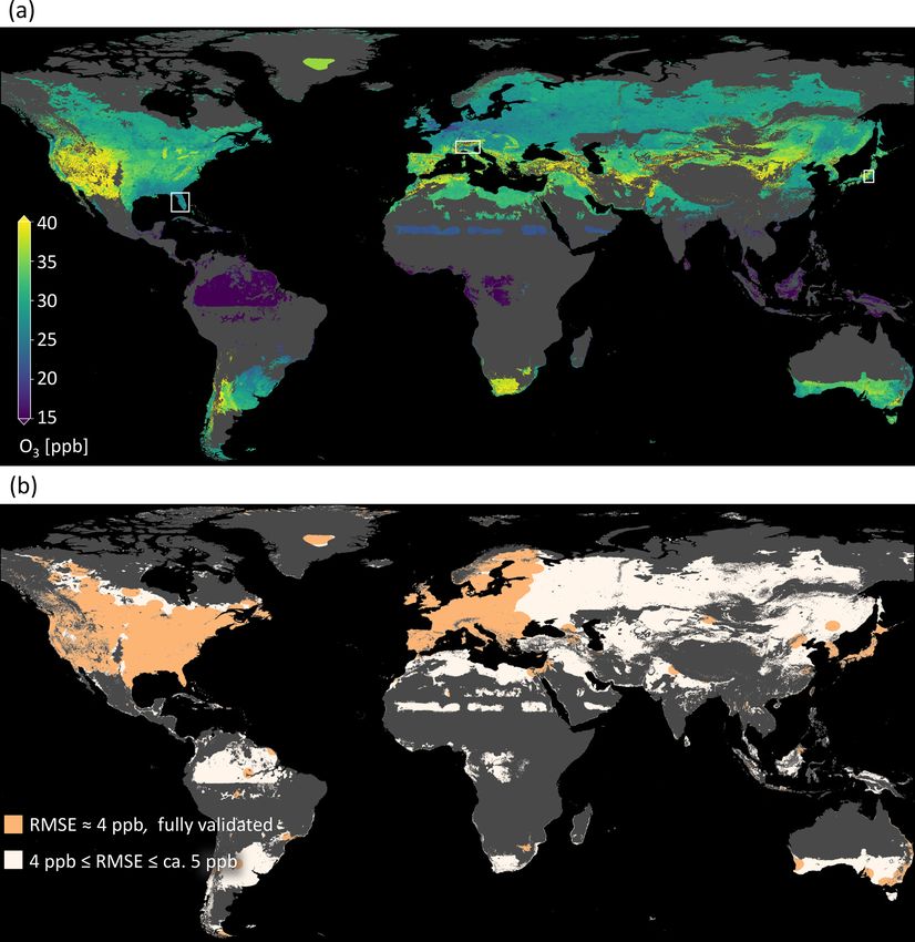
4332                                           C. Betancourt et al.: Global, high-resolution mapping of tropospheric ozone

of these factors of ozone formation, destruction, and trans-       by exploiting similarities between distant sites. In contrast to
port is not fully understood (Schultz et al., 2017). This makes    traditional interpolation techniques, mapping allows to ex-
ozone both difficult to quantify and to control. Public au-        tend the domain to the global scale, because it can predict
thorities recognize ozone-related problems. They install air       the variable of interest based on environmental features, even
quality monitoring networks to quantify ozone (Schultz et al.,     in regions without measurements (Lary et al., 2014; Bastin
2015, 2017). Furthermore, they enforce maximum exposure            et al., 2019; Hoogen et al., 2019). Recently, it is questioned
rules to mitigate ozone health and vegetation impacts (e.g.,       whether machine learning methods are the most suitable to
European Union, 2008).                                             “map the world” (Meyer, 2020): Meyer et al. (2018) and Plo-
   Currently, there is increased use of machine learning meth-     ton et al. (2020) point out that some studies may be overcon-
ods in tropospheric ozone research. Such “intelligent” al-         fident because they validate their maps on data that are not
gorithms can learn nonlinear relationships of ozone pro-           statistically independent from the training data. This occurs
cesses and connect them to environmental conditions, even if       when a random data split is used on data with spatiotem-
their interrelations are not well understood through process-      poral (auto)correlations. There are also concerns when the
oriented research. Kleinert et al. (2021) and Sayeed et al.        mapping models are applied to areas that have completely
(2021) used convolutional neural networks to forecast ozone        different properties from the measurement locations (Meyer
at several hundred measurement stations, based on meteoro-         and Pebesma, 2021). A model trained on certain input feature
logical and air quality data. Large training datasets allowed      combinations can only be applied to similar feature combi-
them to train deep neural networks, resulting in a significant     nations. Furthermore, uncertainty estimates of the produced
improvement over the first machine learning attempts to fore-      maps are important as they are often used as a basis for fur-
cast ozone (Comrie, 1997; Cobourn et al., 2000). Machine           ther research.
learning is also used to calibrate low-cost ozone monitors that       In this study, we produce the first fully data-driven global
complement existing ozone monitoring networks (Schmitz             map of tropospheric ozone, aggregated in time over the years
et al., 2021; Wang et al., 2021). Furthermore, compute-            2010–2014. This study builds upon Betancourt et al. (2021b)
intensive chemical reactions schemes for numerical ozone           who proved that ozone metrics can be predicted using static
modeling can be emulated using machine learning (Keller            geospatial data. We provide the map as a product and com-
et al., 2017; Keller and Evans, 2019). Ozone datasets which        bine it with uncertainty estimates and explanations to ensure
are used as training data for machine learning models are in-      the trustworthiness of our results. We justify the choice of
creasingly made available as FAIR (Wilkinson et al., 2016)         methods and clarify why they are necessary for a thorough
and open data. AQ-Bench (“air quality benchmark dataset”,          global analysis. Section 2 contains a description of the data
Betancourt et al., 2021b), for example, is a dataset for ma-       and machine learning methods, including explainable ma-
chine learning on global ozone metrics and serves as training      chine learning and uncertainty estimation. Section 3 contains
data for this mapping study.                                       the results, which are discussed in Sect. 4. We conclude in
   We refer to mapping as a data-driven method for spa-            Sect. 5.
tial predictions of environmental target variables. For map-
ping, a model is fit to observations of the target variable at
measurement sites, which might even be sparse and irreg-           2     Data and methods
ularly placed. Environmental features are used as proxies
                                                                   2.1     Data description
for the target variable to fit the model. A map of the tar-
get variable is produced by applying the model to the spa-         In this section, we present the datasets used in this study.
tially continuous features in the mapping domain. Mapping          Technical details on these data are given in Appendix A.
for environmental applications has been performed since the
1990s (Mattson and Godfrey, 1994; Briggs et al., 1997). It         2.1.1    AQ-Bench dataset
was deployed for air pollution as an improvement over spa-
tial interpolation and dispersion modeling, which suffer from      We fit our machine learning model on the AQ-Bench dataset
performance issues due to sparse measurements, and lack of         (“air quality benchmark dataset”, Betancourt et al., 2021b).
detailed source description (Briggs et al., 1997). Hoek et al.     The AQ-Bench dataset is a machine learning benchmark
(2008) describe these early mapping studies as “linear mod-        dataset that allows to relate ozone statistics at air qual-
els with little attention to mapping outside the study area”.      ity measurement stations to easy-access geospatial data.
In contrast, modern machine learning algorithms are often          It contains aggregated ozone statistics of the years 2010–
trained on thousands of samples for mapping (Petermann             2014 at 5577 stations around the globe, compiled from
et al., 2021; Heuvelink et al., 2020). Several studies (e.g., Li   the database of the Tropospheric Ozone Assessment re-
et al., 2019; Ren et al., 2020) have shown that mapping using      port (TOAR, Schultz et al., 2017). The AQ-Bench dataset
machine learning methods is superior to other geostatistical       considers ozone concentrations on a climatological time
methods such as Kriging because it can capture nonlinear           scale instead of day-to-day air quality data. The scope of
relationships and makes ideal use of environmental features        this dataset is to discover purely spatial relations. Machine

Geosci. Model Dev., 15, 4331–4354, 2022                                             https://doi.org/10.5194/gmd-15-4331-2022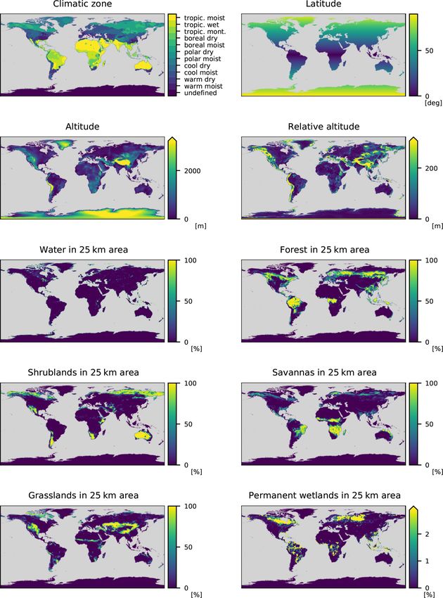
C. Betancourt et al.: Global, high-resolution mapping of tropospheric ozone                                                        4333

Figure 1. Average ozone statistic of the AQ-Bench dataset. The values at 5577 measurement stations are aggregated over the years 2010–
2014. (a) Values on a map projection. (b) Histogram and summary statistics.

learning models trained on this dataset will output aggre-
gated statistics over the years 2010–2014 and will not be
able to capture temporal variances. This is beneficial if the re-
quired final data products are also aggregated statistics. The
majority of the stations are located in North America, Eu-
rope, and East Asia. The dataset contains different kinds of
ozone statistics such as percentiles or health-related metrics.
This study focuses on the average ozone statistic as the tar-
get (Fig. 1).
   The features in the AQ-Bench dataset characterize the
measurement site and are proxies for ozone formation, de-
struction, and transport processes. For example, the “alti-
tude” and “relative altitude” of the station are important prox-
ies for local flow patterns and ozone sinks. “Population den-
sity” in different radii around every station are proxies for hu-
man activity and thus ozone precursor emissions. “Latitude”
is a proxy for ozone formation through photochemistry, as ra-        Figure 2. Predicted ozone values versus measurement values of the
diation and heat generally increase towards the Equator. The         test set of the AQ-Bench dataset. See Sect. 3.3.1 for the specifica-
land cover variables are proxies for precursor emissions and         tions of the used machine learning model.
deposition. The full list of features and their relation to ozone
processes are documented by Betancourt et al. (2021b). Fig-
ure 2 shows predictions of a machine learning model on the           2.2   Explainable machine learning workflow
test set of AQ-Bench. Table 1 lists all features used in this
study.                                                               We apply a standard mapping workflow and extend it with
                                                                     explainable machine learning methods as described in this
2.1.2   Gridded data                                                 section. Together with the uncertainty assessment methods
                                                                     described in Sect. 2.3, they allow for a thorough analysis
Features are needed on a regular grid (i.e., as raster data) over    of our machine learning model. A random forest (Breiman,
the entire mapping domain to map the target average ozone.           2001) is fit on the AQ-Bench dataset to predict average ozone
The original gridded data used here (Appendix Sects. A               for given features. A random forest is an ensemble of regres-
and B) has a resolution of 0.1◦ × 0.1◦ or finer. Since our           sion trees that is created by bootstrapping the training dataset
target resolution is 0.1◦ × 0.1◦ , the gridded data are down-        to increase generalizability. We choose random forest be-
scaled to that resolution if the original resolution is finer.       cause tree-based models are the state of the art for structured
The “land cover”, “population”, and “light pollution” fea-           data (Lundberg et al., 2020). Random forest was also shown
tures of the AQ-Bench dataset are spatial aggregates in a            to outperform linear regression and a shallow neural network
certain radius around the station (see Table 1). To prepare          in predicting average ozone on the AQ-Bench dataset (Be-
gridded fields of these features, the area around each indi-         tancourt et al., 2021b). In addition, this algorithm has been
vidual grid point is considered, and the required radius ag-         proven to be suitable for mapping in several studies (Peter-
gregation is written to that grid point. The gridded dataset         mann et al., 2021; Nussbaum et al., 2018; Ren et al., 2020).
is available under the DOI https://doi.org/10.23728/b2share.         We use the Python framework SciKit-learn (Pedregosa et al.,
9e88bc269c4f4dbc95b3c3b7f3e8512c (Betancourt et al.,                 2011) for machine learning and hyperactive (Blanke, 2021)
2021c).                                                              for hyperparameter tuning.

https://doi.org/10.5194/gmd-15-4331-2022                                                Geosci. Model Dev., 15, 4331–4354, 2022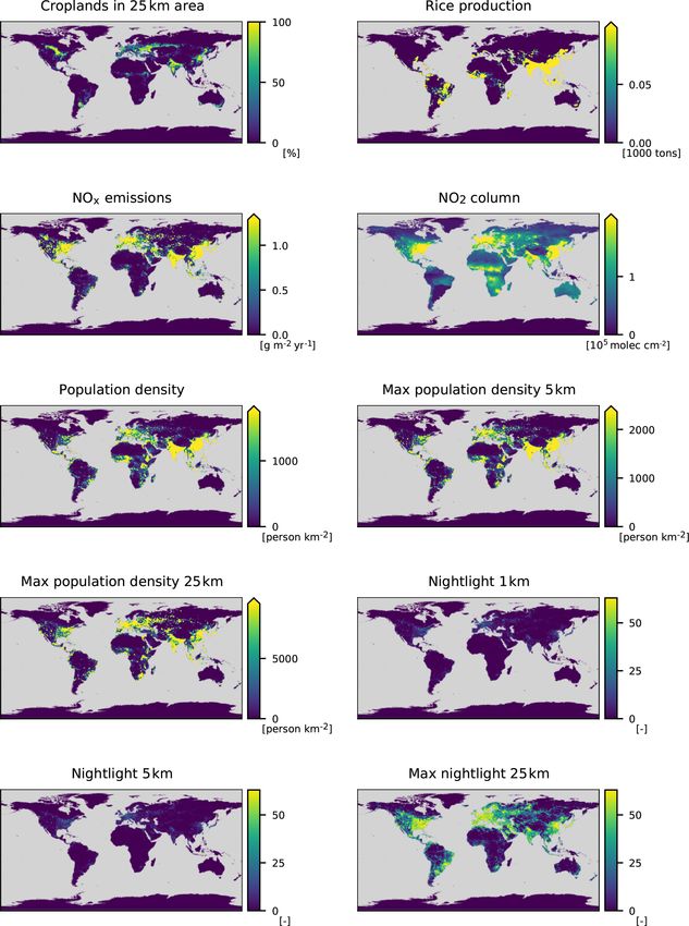
4334                                            C. Betancourt et al.: Global, high-resolution mapping of tropospheric ozone

Table 1. Features selected from the AQ-Bench dataset.

                                            Feature                                            Unit
                       General              Climatic zone                                      –
                                            Latitude                                           ◦
                                            Altitude                                           m
                                            Relative altitude                                  m
                       Land cover           Water in 25 km area                                %
                                            Evergreen needleleaf forest in 25 km area          %
                                            Evergreen broadleaf forest in 25 km area           %
                                            Deciduous needleleaf forest in 25 km area          %
                                            Deciduous broadleaf forest in 25 km area           %
                                            Mixed forest in 25 km area                         %
                                            Closed shrublands in 25 km area                    %
                                            Open shrublands in 25 km area                      %
                                            Woody savannas in 25 km area                       %
                                            Savannas in 25 km area                             %
                                            Grasslands in 25 km area                           %
                                            Permanent wetlands in 25 km area                   %
                                            Croplands in 25 km area                            %
                                            Urban and built-up in 25 km area                   %
                                            Cropland/natural vegetation mosaic in 25 km area   %
                                            Snow and ice in 25 km area                         %
                                            Barren or sparsely vegetated in 25 km area         %
                       Agriculture          Wheat production                                   1000 t yr−1
                                            Rice production                                    1000 t yr−1
                       Ozone precursors     NOx emissions                                      g m−2 yr−1
                                            NO2 column                                         105 molec cm−2
                       Population           Population density                                 person km−2
                                            Maximum population density in 5 km area            person km−2
                                            Maximum population density in 25 km area           person km−2
                       Light pollution      Nightlight in 1 km area                            brightness index
                                            Nightlight in 5 km area                            brightness index
                                            Maximum nightlight in 25 km area                   brightness index

   A proper validation strategy is crucial for spatial predic-        et al. (2018). Additionally, we apply basic feature engineer-
tion models because both environmental conditions and tar-            ing to increase the interpretability of the model. Details on
get variables are often correlated in space. When tested on           feature engineering and feature selection are described in
spatially correlated and thus statistically dependent samples,        Sect. 2.2.2. In order to make our mapping model trustworthy,
mapping results may be overconfident (Meyer et al., 2018;             we verify its robustness and ability to generalize to unseen lo-
Ploton et al., 2020). We use the independent spatial data split       cations, and to explore the limits of its predictive capabilities.
provided with the AQ-Bench dataset to validate spatial gen-           Noise in the AQ-Bench dataset causes problems if the model
eralizability. Details on our validation strategy are given in        is not robust. Additionally, limited availability of ozone mea-
Sect. 2.2.1.                                                          surements in regions like central and southeast Asia, Central
   As an extension of the standard mapping workflow de-               and South America, and Africa poses a problem as it is un-
scribed in Sect. 1, we perform experiments to increase in-            clear whether our model will generalize to these regions. We
terpretability, test robustness, and explain the model. The ex-       address the issues of robustness and generalizability using
tended workflow is summarized in Table 2 and further justi-           the spatial cross-validation strategy described in Sect. 2.2.3.
fied in the following.                                                   We also aim to explain how the model arrives at its pre-
   The use of redundant features in mapping applications can          dictions and check consistency with common ozone pro-
favor spatial overfitting. We thus remove counterproductive           cess understanding by using SHAP (SHapley Additive ex-
features by forward feature selection as proposed by Meyer            Planations, Lundberg and Lee, 2017), a post hoc explainable

Geosci. Model Dev., 15, 4331–4354, 2022                                                https://doi.org/10.5194/gmd-15-4331-2022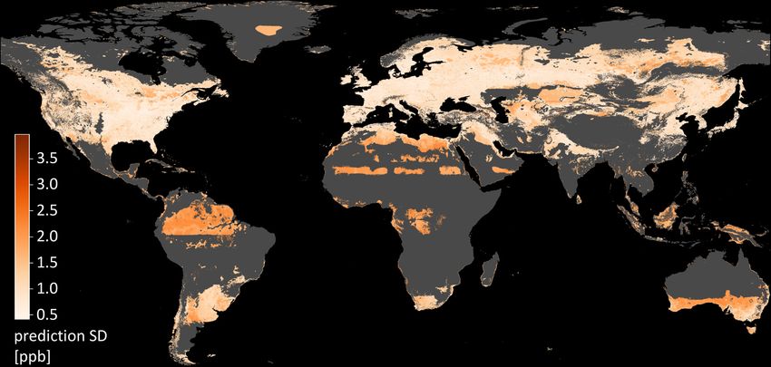
C. Betancourt et al.: Global, high-resolution mapping of tropospheric ozone                                                            4335

Table 2. Machine learning experiments as an addition to the standard mapping method. For details on the methods, refer to the given sections.

                Section    Method                               Goal
                2.2.2      Feature engineering                  Make features easier to interpret
                           Forward feature selection            Remove counterproductive features which favor overfitting
                2.2.3      Spatial cross validation             Check model spatial robustness
                           Cross validation on world regions    Evaluate model generalizability
                2.2.4      Calculate SHAP values                Explain model predictions

machine learning method. It is a game-theoretic approach                 each remaining feature along with the already selected fea-
based on Shapley values (Shapley, 1953). SHAP identifies                 tures. The additional feature with the best evaluation score
the importance of the individual features to a model predic-             is appended to the existing list of features. This iterative ap-
tion (Sect. 2.2.4).                                                      proach is continued until the R 2 value drops, which indicates
                                                                         that a feature leads to overfitting. The selected features are
2.2.1   Evaluation scores                                                presented in Sect. 3.1.1.
We rely on the independent 60 %–20 %–20 % data split of                  2.2.3   Spatial cross validation
AQ-Bench as provided by Betancourt et al. (2021b). Here,
stations with a distance of more than 50 km are considered               We apply cross validation to prove the robustness of our
independent of each other.                                               model. We split the test and training set into four indepen-
   The evaluation score is the coefficient of determina-                 dent cross-validation folds of 20 % each. Like Betancourt
tion R 2 ,                                                               et al. (2021b), we assume that air quality measurement sta-
           PM               2                M                           tions with a distance of at least 50 km are independent of each
  2          m=1 (ym − ŷm )              1 X                            other. We, therefore, produce the cross-validation folds with
R = 1 − PM                     with hyi =       ym ,   (1)
             m=1 (ym − hyi)
                             2            M m=1                          a two-step approach. First, we cluster the data based on the
                                                                         spatial location of the measurement sites using the density-
where m denotes a sample index, M the total number of sam-               based clustering algorithm DBSCAN (Ester et al., 1996).
ples, ŷm a predicted target value, and ym a reference target            The maximum distance between clusters is set to 50 km so
value. R 2 measures the proportion of variance in the output             stations closer than that distance are assigned to the same
values that the model predicts. Thus, a larger R 2 represents            cluster. Small clusters are randomly assigned to the cross-
a better model and the largest possible value is 1. We also              validation folds. In the second step, larger clusters (n > 50)
evaluate the root mean square error (RMSE) in ppb:                       are split with k-means clustering (Duda et al., 2001) to ensure
           v
           u M                                                           the same statistical distribution of all cross-validation folds.
           u X (ym − ŷm )2                                              The resulting smaller clusters are again randomly assigned to
RMSE = t                      .                           (2)
             m=1
                      M                                                  the cross-validation folds. Figure 3a shows this data split.
                                                                            We extend our spatial cross-validation experiment to eval-
2.2.2   Feature engineering and feature selection                        uate the generalizability of our predictions to world re-
                                                                         gions with few measurements. Here, we divide the data into
We perform basic feature engineering to improve the inter-               the three world regions: North America, Europe, and East
pretability of our model. Different types of savanna, shrub-             Asia (Fig. 3b). A random forest is fit and evaluated on two
lands, and forests are given individually in AQ-Bench (Ta-               of the three regions and also evaluated on the third region
ble 1). We merge them into “savanna”, “forest”, and “shrub-              for comparison. For example, it is fit and evaluated on data
land” because a high number of features with similar proper-             of Europe and North America and additionally evaluated in
ties would make the model interpretation more difficult. In-             East Asia. The difference in the resulting evaluation scores
stead of “latitude”, we train on the “absolute latitude”, since          shows the spatial generalizability of the model. The results
radiation and temperature decrease when moving away from                 are presented in Sect. 3.1.2.
the Equator, regardless of whether one moves south or north.
Compared to experiments performed without feature engi-                  2.2.4   SHapley Additive exPlanations
neering, we did not see any change in evaluation scores.
   We use the forward feature selection method for spatial               SHAP (Lundberg and Lee, 2017) provides detailed expla-
prediction models by Meyer et al. (2018). The model is ini-              nations for individual predictions by quantifying how each
tially trained on all two-feature pairs. The pair with the high-         feature contributes to the result. The contribution refers to
est evaluation score is kept. The model is then trained on               the average model output (or base value) over the train-

https://doi.org/10.5194/gmd-15-4331-2022                                                     Geosci. Model Dev., 15, 4331–4354, 2022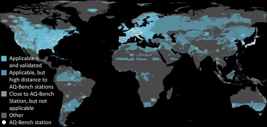
4336                                               C. Betancourt et al.: Global, high-resolution mapping of tropospheric ozone

Figure 3. Data splits for the spatial cross validation. (a) Station clusters are randomly assigned to four cross-validation (CV) folds. (b) The
data are divided by the world regions North America (NAM), Europe (EUR), and East Asia (EAS).

ing set: a feature with the SHAP value x causes the model                 through training instability, the model uncertainty is usually
to predict x more than the base value. We use the Tree-                   high for predictions in areas of the feature space where train-
Shap module (Lundberg et al., 2018) of the Python pack-                   ing data are sparse (Lee et al., 2017; Meyer and Pebesma,
age SHAP (Lundberg and Lee, 2017) to calculate SHAP                       2021). For example, a model that was not trained on data
values. Global feature importance is obtained by adding up                from very high mountains or deserts is not expected to pro-
all local contributions to the predictions. Features with high            duce reliable results in areas with these characteristics. We
absolute contributions are considered more important. The                 apply the concept of “area of applicability” by Meyer and
SHAP values of our model are presented in Sect. 3.1.3.                    Pebesma (2021) to limit our mapping to regions where our
                                                                          model is expected to produce reliable results. The details are
2.3    Methods to assess the impact of uncertainties                      described in Sect. 2.3.1.
                                                                             The target variable “average ozone” is the first choice for
Uncertainty assessment increases the trustworthiness of our               assessment of data errors. Fluctuations and random measure-
machine learning approach and final ozone map. In general,                ment errors introduce uncertainty into the ozone measure-
the predictions of machine learning models have two kinds                 ments. We evaluate the uncertainty introduced by these influ-
of uncertainties (Gawlikowski et al., 2021): first, model un-             ences in the map using a simple error model. The error model
certainty, which results from the trained machine learning                is used to perturb the training data, to check how the map
model itself, and second, data uncertainty which stems from               changes when the model is trained on perturbed data instead
the uncertainty inherent in the data. It is common to treat               of original data. The error model is described in Sect. 2.3.2.
these uncertainties separately. Developing an uncertainty as-                Additional data uncertainty stems from the features. For
sessment strategy for our mapping approach is challenging                 example, geospatial data derived from satellite products are
because different uncertainties arise at different stages of the          sensitive to retrieval errors. Based on the sources and doc-
mapping process. Every ozone measurement, every prepro-                   umentation of our geospatial data (Appendix A), we expect
cessing step, and every model prediction is a potential source            such errors to have a small impact in this study. However, we
of error. It would be infeasible to investigate the impacts of            inspect the subgrid features in the geospatial data and their
every error. We, therefore, identify the most important error             effect on the model results. We limit ourselves to the “al-
sources and analyze the uncertainty induced in our produced               titude” because our SHAP analysis (Sect. 3.1.3) has shown
map only for these. The decision on which aspects to ana-                 that it is the most important feature besides “latitude” which
lyze specifically is based on expert knowledge and the results            does not have critical subgrid variations. Subgrid variations
of our machine learning experiments, i.e., robustness analy-              of the altitude might influence our final map, especially if a
sis (Sect. 2.2.3) and SHAP values (Sect. 2.2.4). We develop               feature like a cliff or a high mountain is present in the respec-
a formalized approach which is summarized in Table 3 and                  tive grid cell. We evaluate the influence of subgrid variations
further elaborated in the following.                                      in altitude on the final map by propagating higher resolution
   The model error is caused by the uncertainty of the train-             altitudes through the final model as described in Sect. 2.3.2.
able parameters of the model. It becomes visible, for exam-
ple, when different results are obtained if the model is ini-             2.3.1   Area of applicability method
tialized with different random seeds before training (Peter-
mann et al., 2021). To rule out this training instability, we re-         We adopt the area of applicability method from Meyer and
trained our models several times with different random seeds              Pebesma (2021). The method is based on considering the dis-
and monitored the results. We found negligible variations and             tance of a prediction sample to training samples in the fea-
thus rule out this kind of uncertainty. Apart from uncertainty            ture space. This concept is illustrated in Fig. 4, where it can

Geosci. Model Dev., 15, 4331–4354, 2022                                                     https://doi.org/10.5194/gmd-15-4331-2022
C. Betancourt et al.: Global, high-resolution mapping of tropospheric ozone                                                           4337

Table 3. Uncertainty assessment for our mapping method. For details on the methods, refer to the given sections.

        Section    Method                                                 Goal
        2.3.1      Define area of applicability                           Ensure the model is only applied where it is reliable
        2.3.2      Modeling of ozone fluctuations                         Evaluate the impact of ozone fluctuations on produced map
        2.3.3      Propagate subgrid altitude variation through model     Evaluate uncertainty introduced by altitude variation

                                                                          map. Such biases may arise from measurement uncertain-
                                                                          ties, local geographic effects, or an “unusual” environment
                                                                          with respect to precursor emission sources. We consider all
                                                                          of these effects as ozone measurement uncertainties although
                                                                          it would be more precise to say that they are uncertainties in
                                                                          the determination of ozone concentrations at the scale of our
                                                                          grid boxes.
                                                                             Quantification of these uncertainties is challenging, as we
                                                                          typically lack the necessary local information. We, therefore,
                                                                          assume the local ozone values are subject to a Gaussian er-
                                                                          ror of mean 0 ppb and variance 5 ppb (Sect. 4, Schultz et al.,
                                                                          2017). We randomly perturb a subset of the training ozone
                                                                          values with this Gaussian error and monitor resulting vari-
                                                                          ances in the final map. Assuming only one-quarter of the
                                                                          measurement values are biased, 25 % of the training ozone
                                                                          values are either increased or decreased by random values
                                                                          in this Gaussian distribution. We use multiple realizations of
Figure 4. Principle of the area of applicability. The plot displays the
                                                                          this error model to perturb the training data, each realization
distribution of all AQ-Bench samples along the three most impor-
tant feature axes “absolute latitude”, “altitude”, and “relative alti-    perturbing a different subset with different values. One ex-
tude”. It is clearly visible that the AQ-Bench samples form a cluster,    ample error model realization is shown in Appendix C.
and that some feature combinations in the gridded data are far away          We train on the randomly perturbed data, obtain a “per-
from this cluster.                                                        turbed model”, and then create “perturbed maps”. If the per-
                                                                          turbations of the resulting ozone maps are less or equal to
                                                                          the initial perturbations, the resulting uncertainty in the map
be clearly seen that the AQ-Bench dataset forms a cluster                 is acceptable. If completely different maps would be pro-
in the feature space, but that our mapping domain contains                duced, this would point to a model lacking robustness. The
feature combinations that do not belong to this cluster. Pre-             process of perturbing, training, and comparing maps is re-
dictions made on these feature combinations suffer from high              peated until the standard deviation of all perturbed maps
uncertainty. Consequently, we mark data points with a great               converges. The error model converged fully after 100 real-
distance to the training data cluster as “not predictable”.               izations (Appendix D). The result of this experiment is pre-
   After we normalized the features, we scaled them accord-               sented in Sect. 3.2.2.
ingly to their global feature importance (Sect. 2.2.4) to in-
crease their respective relevance. We use the cross-validation
sets described in Sect. 2.2.3 to find a threshold distance for            2.3.3   Propagating subgrid altitude variation through
non-predictable samples. In detail, we calculate the distance                     model
from every training data point to the closest data point in
a different cross-validation set. The threshold distance for
“non-predictable” data is the upper whisker of all the cross-             In contrast to perturbing the targets and retraining the ma-
validation distances. Since the model is trained on land sur-             chine learning model, here we sample inputs from a finer res-
face data only, we also remove the oceans from the area                   olution grid and propagate them through the existing trained
of applicability. The result of this experiment is shown in               model. For every grid cell of our final map with 0.1◦ resolu-
Sect. 3.2.1.                                                              tion, we propagate all “altitude” values of the original finer
                                                                          resolution digital elevation model (DEM, resolution 10 , Ap-
2.3.2   Modeling ozone fluctuations                                       pendix A) through our random forest model while leaving
                                                                          the other variables unchanged. For each coarse 0.1◦ resolu-
Here, we describe our error model for evaluating the uncer-               tion grid cell, we find 36 altitude values of the fine grid cells
tainty introduced by typical ozone biases in the produced                 and can thus make 36 predictions. We monitor the deviation

https://doi.org/10.5194/gmd-15-4331-2022                                                    Geosci. Model Dev., 15, 4331–4354, 2022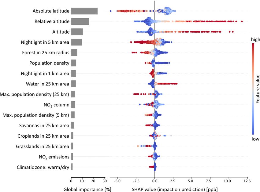
4338                                           C. Betancourt et al.: Global, high-resolution mapping of tropospheric ozone

of these predictions from the reference prediction in that cell.   Table 4. Four-fold cross-validation results.
The results of these experiments are presented in Sect. 3.2.3.
                                                                                   Fold             R2    RMSE [ppb]

3     Results                                                                      1              0.64            3.83
                                                                                   2              0.58            4.03
The results of our explainable machine learning mapping                            3              0.61            4.04
                                                                                   4              0.61            3.97
workflow (Sect. 2.2, Table 2) are presented in Sect. 3.1. The
impact of uncertainties (Sect. 2.3, Table 3) are presented in                      ∅       0.61 ± 0.02     3.97 ± 0.08
Sect. 3.2. The final ozone map that is generated based on
the knowledge gained from all experiments is presented in
Sect. 3.3.                                                           – nightlight in 5 km area, and
3.1     Explainable machine learning model                           – maximum nightlight in 25 km area.

3.1.1    Selected hyperparameters and features                     The following features are discarded because the validation
                                                                   R 2 score decreases when they are used to train the model:
We choose the following standard hyperparameters for our           “urban and built-up in 25 km area”, “cropland/natural vege-
random forest model: 100 trees are fit on bootstrapped ver-        tation mosaic in 25 km area”, “snow and ice in 25 km area”,
sions of the AQ-Bench dataset with a mean square er-               “barren or sparsely vegetated in 25 km area”, and “wheat pro-
ror (MSE) loss function and unlimited depth. The evaluation        duction”. A discussion of why these features are counterpro-
scores found to be insensitive to the choice of hyperparame-       ductive follows in Sect. 4.1.
ters. Therefore, the standard hyperparameters are used to fit
the model in all experiments of this study.                        3.1.2   Spatial cross validation reveals limits in the
   Based on the forward feature selection (Sect. 2.2.2), the               model generalizability
following variables are used to build the model:
                                                                   The four-fold cross validation from Sect. 2.2.3 results in
    – climatic zone,                                               R 2 values in the range of 0.58 to 0.64 and RMSEs in the
                                                                   range of 3.83 to 4.04 ppb (Table 4). These evaluation scores
    – absolute latitude,                                           show that all models are useful despite the variance in evalu-
    – altitude,                                                    ation scores. The mean R 2 score is 0.61 and the mean RMSE
                                                                   is 3.97 ppb. Putting this RMSE value into perspective, 5 ppb
    – relative altitude,                                           is a conservative estimate for the ozone measurement er-
                                                                   ror (Schultz et al., 2017). It is also lower than the 6.40 ppb
    – water in 25 km area,                                         standard deviation of the true ozone values of the training
    – forest in 25 km area,                                        dataset (Fig. 1). Although the evaluation scores of all folds
                                                                   are in an acceptable range, the evaluation scores depend on
    – shrublands in 25 km area,                                    the data split to some extend.
                                                                      If our model is validated on a different region than it has
    – savannas in 25 km area,                                      been trained on, we observe a drop of the R 2 value by 0.13
    – grasslands in 25 km area,                                    to 0.49, while the RMSE increases for two of the three train-
                                                                   ing regions (Table 5). One reason for the change in evalua-
    – permanent wetlands in 25 km area,                            tion scores when training and validating in different world re-
                                                                   gions could be different feature combinations of the different
    – croplands in 25 km area,                                     world regions. We ruled out this reason by inspecting the fea-
    – rice production,                                             ture space (similar to Sect. 2.3.1; not shown). The only other
                                                                   possible reason for the decrease in R 2 is that the relationship
    – NOx emissions,                                               between features and ozone is not the same in different world
                                                                   regions. Therefore, the expected evaluation scores of our map
    – NO2 column,                                                  vary not only with the feature combinations (as described in
    – population density,                                          Sect. 2.3.1) but also spatially. We differentiate between the
                                                                   two issues and their influence on the model applicability in
    – maximum population density in 5 km area,                     Sect. 3.2.1.
    – maximum population density in 25 km area,
    – nightlight in 1 km area,

Geosci. Model Dev., 15, 4331–4354, 2022                                                https://doi.org/10.5194/gmd-15-4331-2022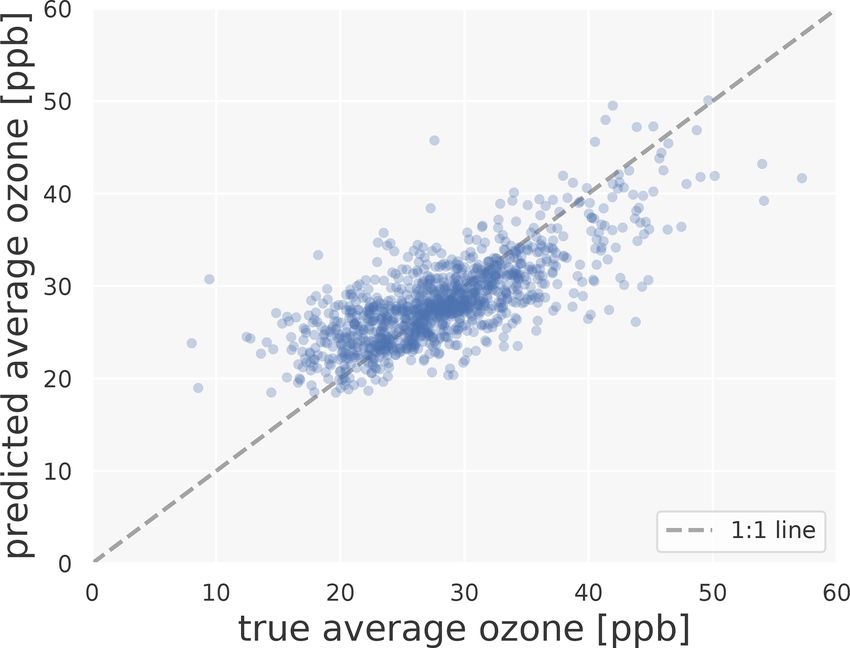
C. Betancourt et al.: Global, high-resolution mapping of tropospheric ozone                                                     4339

Table 5. Cross validation on the world regions Europe (EUR), East Asia (EAS), and North America (NAM). We give the difference in
R 2 values and RMSEs when validating the model in another world region than the training region.

                                 Training region   Validation region               R2    RMSE [ppb]
                                 EUR + EAS         EUR + EAS                     0.57           3.54
                                                   NAM                           0.34           5.01
                                                                        diff.   −0.23          +1.47
                                 EAS + NAM         EAS + NAM                     0.52           3.76
                                                   EUR                           0.39           4.64
                                                                        diff.   −0.13          +0.88
                                 NAM + EUR         NAM + EUR                     0.63           3.92
                                                   EAS                           0.14           3.78
                                                                        diff.   −0.49          −0.14

3.1.3    SHAP values quantify the influence of the                     from both the area of applicability (for matching features)
         features on the model results                                 and the spatial cross-validation methods (for spatial proxim-
                                                                       ity).
SHAP was used to determine the feature importance of the                  Analogously to the approach of the area of applicabil-
random forest model as described in Sect. 2.2.4. Figure 5              ity (Sect. 3.2.1), we analyze the distances between measure-
contains a summary plot with the global feature impor-                 ment stations in the geographical space. To quantify spa-
tance (left side) and SHAP values of all features on the test          tial proximity, we calculate the mean distance of a measure-
set (right side). The global importance of the features “abso-         ment station and its closest neighboring station in a differ-
lute latitude”, “altitude”, “relative altitude”, and “nightlight       ent cross-validation set. Disregarding stations that are too
in 5 km area” are highest with a contribution of at least 10 %.        far away from the others, we identified the distance of ap-
The remaining features have a weaker influence on the model            proximately 182 km (upper whisker), within which we ex-
output. For example, the influence of the “climatic zone” is           pect a comparable RMSE as shown in Table 4. We assume a
often negligible. The local SHAP values in Fig. 5 reveal the           higher RMSE for locations that are more than 182 km away
contribution of features to the predictions. A lower “absolute         from their closest neighboring measurement station. Figure 6
latitude” value leads to an increased ozone value prediction.          shows the area of applicability of our model including this
Likewise, higher “altitude” and “relative altitude” increase           spatial distinction.
predicted ozone values. High “nightlight in 5 km area” values             The majority of the regions with good coverage of mea-
lead to lower predicted ozone concentrations. These tenden-            surement stations (North America, Europe, and parts of
cies are in line with domain knowledge on the atmospheric              East Asia) are well predictable. In these regions, only some
chemistry of ozone. Appendix E shows SHAP values of two                areas in the high north and high mountains are not pre-
individual predictions. We discuss the physical consistency            dictable. Conversely, large areas in South and Central Amer-
of the model based on the SHAP values in Sect. 4.1.                    ica, Africa, far northern regions, and Oceania have feature
                                                                       combinations different from the training data and therefore
3.2     Evaluating the impact of uncertainties                         are not predictable. There are some regions in the Baltic area,
                                                                       South America, Africa, and south Australia where feature
3.2.1    Applicability and uncertainty of the model                    combinations can be predicted by the model, but they are far
         depend on both features and location                          away from the AQ-Bench stations. A broader discussion of
                                                                       the global applicability of our machine learning model fol-
As described in Sect. 2.3.1, predictions of our model are              lows in Sect. 4.3.
valid if the feature combinations are similar to those of the
training dataset. Additionally, the results of the spatial cross       3.2.2    Uncertainty due to ozone fluctuations is within an
validation (Sect. 3.1.2) have shown that the spatial proxim-                    acceptable range
ity to the training locations has an influence on the model
performance and uncertainty. Two cases were examined in                The error model for ozone uncertainties is described in
this section: firstly, the cross-validation sets which are close       Sect. 2.3.2. The R 2 values of the perturbed models varied be-
to each other (RMSE in the range of 4 ppb, as seen in Ta-              tween 0.50 and 0.58. Figure 7 shows the resulting standard
ble 4), and secondly, the cross validation on different world          deviation in the mapped ozone. The assumed ozone fluctua-
regions (RMSE values of up to 5 ppb, as seen in Table 5). In           tions have a higher impact in areas with sparse training data.
our uncertainty assessment, we therefore combine findings              We conclude that our error model does not tend to amplify

https://doi.org/10.5194/gmd-15-4331-2022                                                 Geosci. Model Dev., 15, 4331–4354, 2022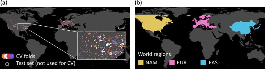
4340                                                 C. Betancourt et al.: Global, high-resolution mapping of tropospheric ozone

Figure 5. SHAP summary plot. The global importance on the left side is calculated from the averaged sum of the absolute SHAP values. The
dots in the beeswarm plots on the right side show the SHAP values of single predictions. The color indicates the respective feature value.
This plot shows only features with more than 1 % global importance.

Figure 6. Area of applicability with restrictions in the feature space and spatial restrictions. The bright turquoise areas fulfill all prerequisites
to be predictable: they have similar features as the AQ-Bench dataset and they are close to stations for validation. The darker shade of
turquoise indicates similar predictions but no proximity to stations for validation. Light gray areas indicate the proximity of a station but no
applicability of the model. The locations of all measurement stations are plotted in white.

the effects of perturbed training data. This means that the                  America. This is because the model relies its predictions on
machine learning algorithm smoothes out noise during train-                  a few samples and is thus sensitive to perturbations of these
ing. This is explained by the core functioning of the random                 few measurements.
forest which uses bootstrapping during training.
   Figure 7 also shows that regions with poor spatial coverage
by measurement stations (darker shade of turquoise in Fig. 6)
are more sensitive to noisy training data. Example regions
are the patches in Greenland, Africa, Australia, and South

Geosci. Model Dev., 15, 4331–4354, 2022                                                         https://doi.org/10.5194/gmd-15-4331-2022
C. Betancourt et al.: Global, high-resolution mapping of tropospheric ozone 4341
Figure 7. Standard deviation of the ozone predictions under perturbations. This map was created by stacking the maps of 100 error model
realizations along the z axis and then calculating the grid point-wise standard deviation along the z axis.
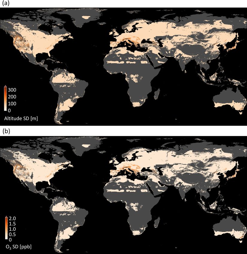
3.2.3 Uncertainty through subgrid DEM variation is 3.3.2 Visual analysis
within an acceptable range
The final map is shown in Fig. 9 (data avail-
able under https://doi.org/10.23728/b2share.
This method was described in Sect. 2.3.3. In most regions
a05f33b5527f408a99faeaeea033fcdc, Betancourt et al.,
of the world, subgrid DEM variations around mean altitude
2021d). Predictions are in a range between 9.4 and 56.5 ppb.
are below 50 m (Fig. 8a), e.g., in the central and eastern
There are some characteristics that are visible at first sight,
United States and in Europe except for the Alps. There are
e.g., higher values in mountain areas, like in the western
regions with higher variances such as the Rocky Mountains
US. The global importance of “absolute latitude” shows
and their surroundings, the Alps, and large parts of Japan
through a latitudinal stratification and a clear north–south
outside Tokyo. In Fig. 8b, it can be seen how these variations
gradient in Europe, the US, and East Asia. Sometimes the
influence the predicted ozone values. In the flat regions, the
borders of climatic zones are visible, like in the north of
variance is below 0.5 ppb, and even in the high-variance re-
North America, and across Asia. This shows that even if the
gions, the deviation is seldom above 2 ppb. This means the
climatic zones are not important globally, they can be locally
model is robust against these variances. Few exceptions are
important. There are larger areas with low ozone variation in
present at the border of the area of applicability (Sect. 3.2.1),
Greenland, Africa, and South America.
e.g., in the Alps. But even in these regions, the deviation is
In Fig. 10, a detailed look at three selected areas is given,
well below 5 ppb. A discussion of implications for general
and the predictions are compared to the true values. In
subgrid variances can be found in Sect. 4.1.
Fig. 10a, a uniform, low ozone concentration is predicted
over the peninsula of Florida. Figure 10b shows low ozone
3.3 The final ozone map values in the Po Valley, a densely populated plane. Towards
the mountains which surround the valley, higher values are
3.3.1 Production of the final map predicted, and for the higher mountains, no predictions can
be made. Figure 10c shows the city of Tokyo, which is cov-
All selected features listed in Sect. 3.1.1 are used to fit the fi- ered with ozone measurements and where ozone values are
nal model. In contrast to the experiments in the previous sec- relatively low. At the coasts of Japan, the values are lower.
tions, we train the model on 80 % of the AQ-Bench dataset The spatial ozone patterns described here can also be found
and test it on the remaining 20 % of the independent test set. in ozone maps generated by traditional chemical models such
Figure 2 shows the predictions on the test set vs. the true as the fusion products by DeLang et al. (2021). We discuss
values. The R 2 value of this model is 0.55 and the RMSE the prospects of global ozone mapping more thoroughly in
is 4.4 ppb. There is a spread around the 1 : 1 line; further- Sect. 4.4.
more, extremes are not captured as well as values closer to
the mean. True values of less than 20 ppb or more than 40 ppb
are predicted with high bias, which is expected since random
forests tend to predict extremes less accurately than values
closer to the mean.
https://doi.org/10.5194/gmd-15-4331-2022 Geosci. Model Dev., 15, 4331–4354, 20224342 C. Betancourt et al.: Global, high-resolution mapping of tropospheric ozone
Figure 8. Results of propagating subgrid DEM variations through the model. (a) Spread of subgrid DEM data. (b) Spread of ozone values.
4 Discussion perturbations, and variances in the map do not exceed our
limit of 5 ppb. Limits in the robustness were only shown
4.1 Robustness through variances above 3 ppb at the borders of the area of
applicability, and in regions with sparse training data (gray
and dark turquoise areas in Figs. 7 and 8). This outcome
Based on Hamon et al. (2020), we define robustness as fol- shows that the issues of applicability (Sect. 4.3) and robust-
lows: The model and map are considered robust if they do ness are interconnected. In areas where the model is applica-
not change substantially under noise or perturbations that ble, it is also more robust and uncertainties are lower.
could realistically occur. We define a 5 ppb change in RMSE In order to make the robustness assessment with respect to
score or predicted ozone values as significant (Schultz et al., data feasible, we strongly reduced the dimensionality of our
2017). Methods to assess the robustness are part of both the error model by using expert knowledge. We conducted two
explainable machine learning workflow (Table 2) and the un- experiments where we modify training data and model in-
certainty assessments (Table 3). Regarding the robustness of puts (Sect. 2.3.2 and 2.3.3). These experimental setups were
the training process, the cross-validation results in Table 4 chosen because they are expected to generalize well. The
show that the model performance depended on the data split. combined robustness experiments have shown that our pro-
This was already noted by Betancourt et al. (2021b) and is duced maps are robust.
regarded as an inherent limitation of a noisy dataset.
We tested the robustness regarding typical variances in the 4.2 Scientific consistency
ozone and geospatial data. The results from Sect. 3.2.2 and
3.2.3 show that the produced ozone map is robust against We discuss the scientific consistency of our model by assess-
these fluctuations. The variances are never above the initial ing the results of the explainable machine learning work-
Geosci. Model Dev., 15, 4331–4354, 2022 https://doi.org/10.5194/gmd-15-4331-2022C. Betancourt et al.: Global, high-resolution mapping of tropospheric ozone 4343 Figure 9. The final ozone map as produced in this study. Panel (a) shows the ozone values; (b) shows the uncertainty estimates. The areas shown in Fig. 10 are highlighted by white boxes. Figure 10. Map details with true values are given as white circles. (a) The Florida peninsula, USA. (b) The Po Valley in northern Italy. (c) Tokyo, Japan, and its surroundings. flow (Table 2). We interpret the selected features, their im- understanding of ozone processes. This is a pure a posteriori portance, and their influence on the model predictions. The approach, meaning we did not in any way enforce scientific features are proxies to ozone processes, which makes it chal- consistency during the training process. lenging to interpret the underlying chemical processes. Nev- Regarding the global feature importance of SHAP (Fig. 5), ertheless, the connections between the features can be dis- it might be counterintuitive that the model focuses more on cussed, if they are plausible and consistent with respect to our geographical features such as “absolute latitude” and “alti- https://doi.org/10.5194/gmd-15-4331-2022 Geosci. Model Dev., 15, 4331–4354, 2022
4344                                           C. Betancourt et al.: Global, high-resolution mapping of tropospheric ozone

tude” than chemical factors such as the “NO2 column”, and          ies for human activity, but are available at higher resolution.
“NOx emissions”. Geographic features are proxies for flow          Similarly, the feature “cropland/natural vegetation mosaic in
patterns and heat, not for ozone chemistry, which would be         25 km area” was discarded because ozone is affected differ-
expected to be more important. This contradiction is due to        ently by croplands and natural vegetation. Together with the
the fact that the model provides an as-is view of ozone con-       large area considered, this feature becomes obsolete. We sus-
centration and is not process oriented in any way. Many fea-       pect the features “snow and ice in 25 km area”, “barren or
tures such as “nightlight” and “population density” are corre-     sparsely vegetated in 25 km area”, and “wheat production”
lated, so retraining the model might swap dependence in the        did not contribute to the model generalizability because they
SHAP values as noted by Lundberg et al. (2020).                    are simply not represented well in the training data. A feature
   The beeswarm plot in Fig. 5 shows the physical consis-          may be an important proxy for ozone, but if the relationship
tency of our model. The effect of “absolute latitude” on pre-      is not expressed in the training data, it cannot be learned by a
dictions is consistent with known ozone formation processes;       machine learning model. This feature can become more im-
i.e., ozone production generally increases when more sun-          portant if other training locations are included. This shows
light is available. This is also evident in the latitudinally      that the placing of measurement locations is crucial.
stratified ozone overview plots in global measurement-based
studies such as TOAR health and TOAR vegetation (Flem-             4.3   Mapping the global domain
ing et al., 2018; Mills et al., 2018). Ozone is affected by
meteorology (temperature, radiation) and precursor emis-           The model has to generalize to unseen locations for global
sions (Sect. 1). The fact that there is no continuous increase     mapping. Two prerequisites are (1) the model must have
of ozone towards tropical latitudes shows that the mapping         seen the feature combination during training; (2) the con-
model at least qualitatively captures the influence of low pre-    nection between features and the target, ozone, must be the
cursor emissions in the tropics. The importance of “abso-          same. The two conditions are only fulfilled in a strictly con-
lute latitude” also indicates that the model can be improved       strained space, as shown in Fig. 6. We combined cross valida-
by including temperature and radiation features from mete-         tion with an inspection of the feature space to ensure match-
orological data. High “relative altitude” and “altitude” both      ing feature combinations. Then, based on the cross valida-
increase the predicted ozone. These relations are consistent       tion on different world regions, we point out regions with
with Chevalier et al. (2007). There are relatively important       sparse or no training data, where higher model errors are ex-
chemistry-related features. We see that high values of “night-     pected (Sect. 3.2.1). We also conducted spatial cross valida-
light in 5 km area” reduce the predicted ozone. This is con-       tion with a shallow neural network (as in the baseline exper-
sistent with NO titration (Monks et al., 2015). Nightlights        iments of Betancourt et al., 2021b). The neural network had
are a proxy for human activity, generally in the context of        similar evaluation scores on the test set but did not general-
fossil fuel combustion, which leads to elevated NOx con-           ize to other world regions, even showing negative R 2 values
centrations. NO destroys ozone, and especially during the          when evaluated in other world regions. We decided to dis-
night time this leads to ozone levels close to zero ppb. High      card the neural network architecture, because our main goal
“forests in 25 km area” values lead to lower ozone predic-         is global generalizability.
tions. This is plausible because there is little human activ-         We can confidently map Europe, large parts of the US and
ity in forested areas and thus no combustion-related precur-       East Asia, where the majority of the measurement stations
sor emissions occur. Quantification of either influence is not     are located. Those are industrialized countries in the north-
possible because, for example, it is unclear to what extent the    ern hemisphere. The cross-validation results (Sect. 3.1.2), the
different forests emit volatile organic compounds which are        area of applicability (Sect. 3.2.1), and expert knowledge con-
also ozone precursors. A city with “nightlight in 5 km area”       firm that uncertainties increase when a model trained on the
equal to 50 cannot be directly quantified in terms of precur-      AQ-Bench dataset is applied to other world regions. How-
sor emissions either. It is also not expected that the machine     ever, the cross validation in connection with the area of appli-
learning model learns the ozone-related processes described        cability technique shows that the model can be used in other
above because it is not process based. Instead, it learns the      world regions with acceptable uncertainties. That is promis-
effects of processes if they are reflected in the training data.   ing for future global mapping approaches. One idea to solve
   The forward feature selection (Sects. 2.2.2 and 3.1.1) can      these problems of different connections between features and
also be discussed in terms of plausibility. Features selected      ozone in different world regions is to train localized models,
by this method favor a generalizable model. Discarded fea-         and apply them wherever possible. Localized models could
tures may help to characterize the locations, but their addi-      not only yield more accurate predictions but in connection
tion to the training data does not lead to a more generaliz-       with SHAP values (Sect. 2.2.4), they could also rule out the
able model. “Urban and built-up in 25 km area” was not se-         governing factors of ozone in the respective regions and be
lected presumably because urban areas are often localized.         easier to interpret.
This feature is therefore not as meaningful as the variables          With regard to the spatial domain, we can also discuss the
“nightlight” and “population density”, which are also prox-        resolution. The model was trained on point data of the “ab-

Geosci. Model Dev., 15, 4331–4354, 2022                                            https://doi.org/10.5194/gmd-15-4331-2022
C. Betancourt et al.: Global, high-resolution mapping of tropospheric ozone                                                 4345

solute latitude”, “altitude”, and “relative altitude”, and one    5   Conclusions
could produce more fine-grained maps if the gridded data
are present in higher resolution. However, one may need           In this study, we developed a completely data-driven,
to reconsider some assumptions made here in terms of re-          machine-learning-based global mapping approach for tropo-
gional representativity of the measurements and the relation      spheric ozone. We mapped from the 5577 irregularly placed
between geographic features and ozone on a different scale.       measurement stations of the AQ-Bench dataset (Betancourt
                                                                  et al., 2021b) to a regular 0.1◦ × 0.1◦ grid. We used a multi-
                                                                  tude of geospatial datasets as input features. To our knowl-
4.4   Prospects for ozone mapping                                 edge, this is the first completely data-driven approach to
                                                                  global ozone mapping. We combined this mapping with an
We mapped average tropospheric ozone from the stations            end-to-end approach for explainable machine learning and
in the AQ-Bench dataset to a global domain. For this, we          uncertainty estimation. This allowed us to assess the robust-
fused different auxiliary geospatial datasets and gridded data    ness, scientific consistency, and global applicability of the
with machine learning. We used features that are known            model. We linked interpretation tools with domain knowl-
proxies for ozone processes, and that were already proven         edge to obtain application-specific explanations, which is in
to enable a prediction of ozone concentrations (Betancourt        line with Roscher et al. (2020). The methods are intercon-
et al., 2021b). Our choice of data and algorithms is well jus-    nected; e.g., forward feature selection made the model easier
tified and transparent. Errors did not exceed 5 ppb, which is     to interpret. Likewise, the area of applicability was shown to
an acceptable uncertainty. The R 2 value of the final model       match the model’s robustness. We justified the choice of tools
is 0.55, which is a good value for properly validated map-        and detailed how they provided us with the results to make a
ping. The maps produced show known patterns of ozone              comprehensive global analysis. The combination of explain-
such as lower levels in metropolitan areas and higher lev-        able machine learning and uncertainty quantification makes
els in Mediterranean or mountainous regions. However, ex-         the model and outputs trustworthy. Therefore, the map we
tremes (Fig. 2) are predicted with higher bias. This can be       produced provides information on global ozone distribution
considered as a general problem of machine learning (Guth         and is a transparent and reliable data product.
and Sapsis, 2019) but was also noted in other ozone modeling         We explained the outcome and the model, which can lead
studies (Young et al., 2018).                                     to new scientific insights. Mapping studies like ours could
    For this first approach, we limited ourselves to the static   also contribute to studies like Sofen et al. (2016) that propose
mapping of aggregated mean ozone. An advantage of this            locations for new air quality measurement sites to extend
approach is that the model result is directly the ozone met-      the observation network. Here, the inspection of the feature
ric of interest (in this case, average ozone). Since the AQ-      space helps to cover not only spatial world regions but also
Bench dataset contains other ozone metrics, they could be         air quality regimes and areas with diverse geographic char-
mapped as well. For example, vegetation- or health-related        acteristics. Building locations can also be proposed based
ozone metrics can be mapped with the same workflow as de-         on their contribution to maximizing the area of applicabil-
scribed here. Another advantage is that we used a multitude       ity (Stadtler et al., 2022). The map as a data product can also
of inputs that could not be used in a traditional model because   be used to refine studies like TOAR (Fleming et al., 2018;
their connection to ozone is unknown. This means we exploit       Mills et al., 2018) because it enables analyzing locations with
two benefits of machine learning: first, obtaining a bias-free    no measurement stations.
estimate of the target directly, and second, using a multitude       It would be beneficial to add time-resolved input features
of inputs with unknown direct impact on the target.               to the training data to improve evaluation scores and increase
    Our model is only valid for the training data period (2010–   the temporal resolution of the map. Adding training data
2014), and it is not suitable to predict ozone values in other    from regions like East Asia, or new data sources such as Ope-
years. Our data product is a map that is aggregated in time.      nAQ (https://openaq.org/, last access: 2 November 2021),
This could be a limitation as sometimes the data product          would close the gaps in the global ozone map.
of interest is a seasonal aggregate or even maps of daily or
hourly air pollutant concentrations. The use of meteorolog-
ical data as static or non-static inputs can be beneficial to
further increase model performance and allow time-resolved
mapping. We applied a completely data-driven approach, re-
lying heavily on geospatial data. The other side of the spec-
trum is DeLang et al. (2021), who fused chemical transport
model output to observations without exploiting the connec-
tion to other features. A possible direction to go from here is
described by Irrgang et al. (2021), who propose the fusion of
models and machine learning to benefit from both methods.

https://doi.org/10.5194/gmd-15-4331-2022                                            Geosci. Model Dev., 15, 4331–4354, 2022
You can also read