Use of genetic algorithms for ocean model parameter optimisation: a case study using PISCES-v2_RC for North Atlantic particulate organic carbon
←
→
Page content transcription
If your browser does not render page correctly, please read the page content below

Development and technical paper
Geosci. Model Dev., 15, 5713–5737, 2022
https://doi.org/10.5194/gmd-15-5713-2022
© Author(s) 2022. This work is distributed under
the Creative Commons Attribution 4.0 License.

Use of genetic algorithms for ocean model parameter
optimisation: a case study using PISCES-v2_RC for
North Atlantic particulate organic carbon
Marcus Falls1 , Raffaele Bernardello1 , Miguel Castrillo1 , Mario Acosta1 , Joan Llort1 , and Martí Galí1,2
1 Department     of Earth Sciences, Barcelona Supercomputing Center, Barcelona, Catalonia, Spain
2 Institut   de Ciències del Mar, ICM-CSIC, Barcelona, Catalonia, Spain

Correspondence: Marcus Falls (marcuspfalls@gmail.com) and Martí Galí (mgali@icm.csic.es)

Received: 28 June 2021 – Discussion started: 6 August 2021
Revised: 23 May 2022 – Accepted: 22 June 2022 – Published: 22 July 2022

Abstract. When working with Earth system models, a con-             tions are recommended to establish the validity of the results
siderable challenge that arises is the need to establish the set    obtained.
of parameter values that ensure the optimal model perfor-
mance in terms of how they reflect real-world observed data.
Given that each additional parameter under investigation in-
creases the dimensional space of the problem by one, simple
brute-force sensitivity tests can quickly become too compu-         1   Introduction
tationally strenuous. In addition, the complexity of the model
and interactions between parameters mean that testing them          The field of Earth science has garnered much interest in re-
on an individual basis has the potential to miss key informa-       cent years due to anthropogenic-driven climate change and
tion. In this work, we address these challenges by develop-         the increasing urgency to implement policies and technolo-
ing a biased random key genetic algorithm (BRKGA) able to           gies to mitigate its effects. As a result, Earth system mod-
estimate model parameters. This method is tested using the          els (ESMs) have become a fundamental tool for studying the
one-dimensional configuration of PISCES-v2_RC, the bio-             impact of shifting climate dynamics and global biogeochem-
geochemical component of NEMO4 v4.0.1 (Nucleus for Eu-              ical cycles (Eyring et al., 2016; Anav et al., 2013; Flato,
ropean Modelling of the Ocean version 4), a global ocean            2011). Driven by the necessity of policymakers to have in-
model. A test case of particulate organic carbon (POC) in the       creasingly reliable future climate projections, ESMs are be-
North Atlantic down to 1000 m depth is examined, using ob-          ing continuously developed, resulting in highly complex and
served data obtained from autonomous biogeochemical Argo            computationally demanding tools. Nevertheless, climate pro-
floats. In this case, two sets of tests are run, namely one where   jections produced by ESMs are still hampered by both tech-
each of the model outputs are compared to the model outputs         nical limitations and a lack of knowledge of important pro-
with default settings and another where they are compared           cesses (Seferian et al., 2020; Henson et al., 2022). Particu-
with three sets of observed data from their respective regions,     larly, the representation of the global carbon cycle, specifi-
which is followed by a cross-reference of the results. The re-      cally ocean biogeochemistry, suffers from many uncertain-
sults of these analyses provide evidence that this approach         ties. Moreover, the drive for realistic physical processes is
is robust and consistent and also that it provides an indica-       pushing ESMs towards a higher spatial resolution, making
tion of the sensitivity of parameters on variables of interest.     the cost of calibrating the ocean biogeochemical component
Given the deviation in the optimal set of parameters from the       (and other components of ESMs) unsustainable (Galbraith
default, further analyses using observed data in other loca-        et al., 2015; Kriest et al., 2020). Thus, there is a vital need
                                                                    for novel solutions that allow the optimisation of such com-
                                                                    ponents in a cost-effective way in order to provide critical

Published by Copernicus Publications on behalf of the European Geosciences Union.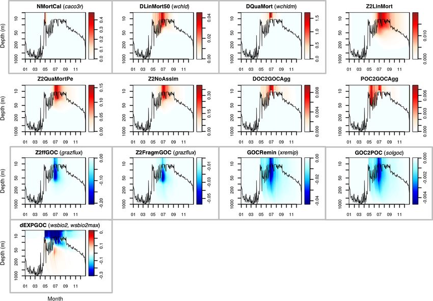
5714                                     M. Falls et al.: Use of genetic algorithms for ocean model parameter optimisation

analyses of the evolution of the climate and answer key soci-      exploration of the parameter space at a reduced computing
etal questions in relation to it (Palmer, 1999, 2014).             cost.
   The tool presented here can be applied to any ESM com-             Attempting to constrain parameters using optimisation
ponent, although this work focuses on ocean biogeochem-            techniques can be difficult in situations of inadequate data
istry because of the many unconstrained parameters that are        or computing power (Matear, 1995; Fennel et al., 2000).
usually needed to numerically represent this realm of the          However, in recent years, this approach has become more
Earth system. In particular, we focus on key biogeochemical        viable within the scientific community due to improvements
processes that contribute to the oceans’ capacity to absorb        in high-performance computing (HPC) techniques that effi-
carbon dioxide from the atmosphere and potentially store it.       ciently exploit the parallelism of supercomputers (Casanova
These processes, usually referred to as the biological carbon      et al., 2011; Broekema and Bal, 2012). These advances fa-
pump, are dominated by the vertical transport of organic mat-      cilitate the running of multiple simulations in parallel, open-
ter from the surface of the ocean to deeper layers (Boyd et al.,   ing the way to efficiently apply PO methods to better un-
2019). This organic matter is exported mostly in the form of       derstand and improve model accuracy. For instance, genetic
detrital particles, which are partly decomposed back to inor-      algorithms (GAs), a particular type of optimisation tech-
ganic carbon and nutrients by bacteria as they sink, and are       nique, can and have been applied to many global search prob-
also transformed by zooplankton. The interplay between bi-         lems and have also started to be used to optimise numeri-
ological processes and sinking determines how long this car-       cal weather models (Oana and Spataru, 2016) and OBGCMs
bon will be stored in the ocean. Given that the oceans have        (Ayata et al., 2013; Ward et al., 2010; Shu et al., 2022). An-
absorbed around 30 % of the carbon dioxide released by hu-         other approach is the training of surrogate models (e.g. using
man activity since preindustrial times (Gruber et al., 2019),      neural networks) from a large set of simulations, enabling
constraining uncertainties in these biogeochemical processes       global sensitivity analyses at reduced computational cost, as
is crucial to predict the future evolution of the climate sys-     done by the Uranie tool (Gaudier, 2010). What these different
tem. However, their representation in models is still a chal-      algorithms have in common is the fact that they are based on
lenge, in particular in the mesopelagic layer that extends         iterative processes traversing a search space by applying op-
between the bottom of the sunlit upper ocean and 1000 m,           erations on the candidate solutions with the purpose of find-
where around 90 % of detrital matter degradation takes place       ing a global optimum. Candidate solutions are evaluated by a
(Burd et al., 2010; Henson et al., 2022).                          fitness function to evaluate their performance in the solution
   Ocean biogeochemistry models (OBGCMs) simplify the              domain.
complexity of the real world by representing biological pro-          This paper documents the application of a genetic algo-
cesses with empirical functions (Fasham et al., 1990), which       rithm to determine an ideal set of parameters that accu-
are parameterised based on laboratory experiments (Pahlow          rately simulate the behaviour of the biogeochemical compo-
et al., 2013) and sparse field measurements (Friedrichs et al.,    nent (PISCES-v2_RC) of an ocean model. The overall aim
2007; Aumont et al., 2015). Therefore, it is likely that model     of this investigation is to demonstrate that using computa-
parameterisations do not reflect the complexity and diversity      tional intelligence techniques, a biased random key genetic
present in our oceans.                                             algorithm (BRKGA) in our case, for parameter estimation
   In the effort to achieve simple yet universally applicable      in Earth system models is an effective approach and to ex-
models, parameter optimisation (PO) techniques are a key           plore, via a BRKGA, how this can be implemented. We also
tool, as they provide an objective means to find a model pa-       describe how to implement a BRKGA and how to embed it
rameter set that produces outputs that match well with ob-         in a state-of-the-art ocean model using a workflow manager
served datasets. However, PO (often referred to as tuning)         (Manubens-Gil et al., 2016).
has traditionally been a rather subjective process, in that
the model developers choose the best parameter sets from
a somewhat comprehensive array of alternative model runs.          2   Methodology
Such subjective optimisation often relied on sensitivity anal-
yses, whereby the variations in model output variables, and        This section outlines the main methods used in this inves-
their skill, were quantified by perturbing one parameter at        tigation. A test case of particulate organic carbon (POC) in
a time. Given the high computational cost of 3D OBGCM              the North Atlantic down to 1000 m is used. The observed
simulations, subjective criteria are still widely used to opti-    data, explained in detail in Sect. 2.1, are obtained from au-
mise OBGCMs. A promising alternative is to perform PO us-          tonomous ocean Argo floats. The model tested is the one-
ing one-dimensional (1D) model configurations, which deal          dimensional (depth) configuration of the ocean biogeochem-
only with local sources and sinks and vertical fluxes along        ical model PISCES-v2_RC (Aumont et al., 2015, 2017), a
the water column (Fasham et al., 1990; Friedrichs et al.,          component of NEMO4 v4.0.1 (Nucleus for European Mod-
2007; Bagniewski et al., 2011; Ayata et al., 2013). Optimis-       elling of the Ocean version 4), as outlined in Sect. 2.2.
ing OBGCMs in 1D is advantageous as it enables a thorough             The type of GA used is BRKGA (Goncalves and Resende,
                                                                   2011). The outline of this method, including the crossover,

Geosci. Model Dev., 15, 5713–5737, 2022                                            https://doi.org/10.5194/gmd-15-5713-2022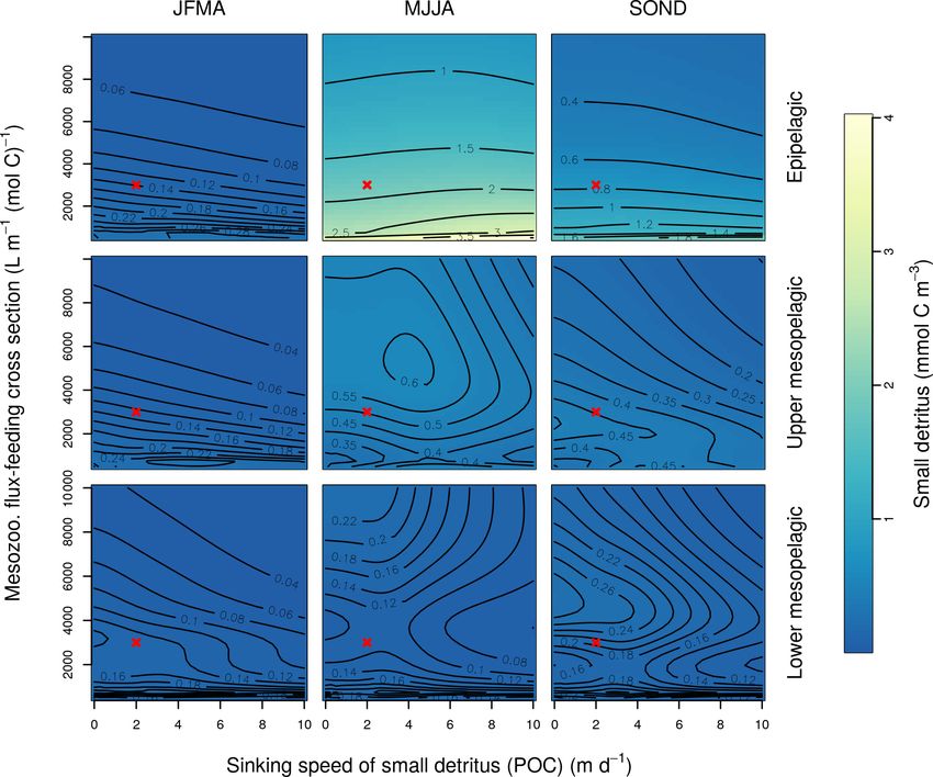
M. Falls et al.: Use of genetic algorithms for ocean model parameter optimisation                                          5715

is described in Sect. 2.3. We use the workflow manager Au-            Finally, we matched the trajectory of the float on a given
tosubmit (Manubens-Gil et al., 2016; Uruchi et al., 2021) to       year to the NEMO model ORCA1 grid (ca. 1◦ horizontal res-
create a workflow that facilitates the various steps of the al-    olution), and chose the ORCA1 grid cell with the best corre-
gorithm, as outlined in Sect. 2.4.                                 spondence between the mixed layer depth observed by the
   This paper outlines two test case experiments in which the      float and that simulated by NEMO (see the next section),
reference data are an output of a simulation with default pa-      hence treating the float as if it sampled a fixed location.
rameters, another three in which the reference data are ob-
served data from three locations in the North Atlantic, and,
                                                                   2.2   PISCES 1D and parameters
last, a set of cross-experiments. Section 2.5 outlines the de-
tails of these experiments.
                                                                   PISCES-v2 (Aumont et al., 2015) is an OBGCM of inter-
2.1   Biogeochemical data                                          mediate complexity that represents the cycles of the main
                                                                   inorganic nutrients (N, P, Si, and Fe), carbonate chemistry,
Our investigation focuses on the vertical profiles of POC in       and organic matter compartments, including phytoplankton
the Labrador Sea region of the North Atlantic subpolar gyre.       and zooplankton organisms (with two size classes each), dis-
The observed data were acquired by Argo floats deployed in         solved organic matter, and particulate organic matter, making
the context of the international Argo programme (Roemmich          up 24 prognostic variables or tracers in total. Here we use a
et al., 2019). Argo floats are autonomous drifting floats fitted   model version, PISCES-v2_RC, that incorporates the POC
with sensors that provide real-time updates of ocean data.         reactivity continuum parameterisation (Aumont et al., 2017).
Over regular intervals, each float rises from its drifting depth   This model version is included as the OBGCM component
of 1000 m to the surface, taking measurements in the process.      of NEMO4 v4.0.1 (Madec et al., 2022) and will hereafter be
When it reaches the surface, it transmits the measurements.        referred to as PISCES.
Initially, the Argo programme focused on observing salin-             In PISCES, detrital POC is represented by two tracers, i.e.
ity and temperature but, more recently, has included biogeo-       POC for detritus smaller than 100 µm and GOC for detri-
chemical measurements (Claustre et al., 2020). Our inves-          tus larger than 100 µm. To avoid confusion between PISCES
tigation focuses on the data of two floats deployed by the         tracers and the term POC, used here as a generic concept
project remOcean and identified by World Meteorological            and to refer to observations, PISCES tracer names are ital-
Organisation numbers 6901486 and 6901527. These floats             icised. It is important to note that total POC as sampled in
took measurements every 1–3 d during times of high biolog-         situ is made up of detrital matter and living biomass. There-
ical activity (i.e. phytoplankton blooms) and every 10 d for       fore, the correspondence between PISCES tracers and ob-
the rest of the year.                                              servations must be established. Here we define SPOC as the
   To enable comparison between biogeochemical (BGC)–              sum of the PISCES tracers for nanophytoplankton (PHY),
Argo data and model simulations, we developed a frame-             microphytoplankton (PHY2), microzooplankton (ZOO) and
work that is described in detail in the companion paper by         small detritus (POC), and LPOC as the sum of large detritus
Galí et al. (2022). Briefly, particulate backscattering mea-       (GOC) and mesozooplankton (ZOO2). These idealised frac-
surements acquired by Argo floats were converted to POC            tions show good correspondence with those determined from
using depth-dependent empirical conversion factors and sep-        BGC–Argo data (Galí et al., 2022). It is important to keep in
arated into two size fractions, small POC (SPOC) and large         mind that detrital POC is a variable proportion of total POC,
POC (LPOC), following Briggs et al. (2020). SPOC cor-              which generally increases with depth. In the mesopelagic, de-
responds to particles smaller than ca. 100 µm that are sus-        trital POC represents around 70 % of total POC globally with
pended or sink slowly, approximately less than 10 m d−1 ,          the default PISCES parameterisation (Table 3 in Galí et al.,
and LPOC corresponds to particles larger than 100 µm whose         2022).
sinking rates are typically of the order of several tens or hun-      Our study focuses on nine PISCES parameters (Table 1)
dreds of metres per day. For each float, we selected one or        expected to strongly influence mesopelagic POC dynamics
more periods of 1 year that were deemed representative of          according to model equations (Aumont et al., 2015, 2017)
the annual cycle in our study region.                              and preliminary analyses (Appendix A and B). These param-
                                                                   eters control POC formation in the surface productive layer
  – LAB1 – float 6901527, year 2016, and −46.2◦ W,                 through microphytoplankton mortality, gravitational POC
    57.2◦ N.                                                       fluxes, POC degradation rates, and interception and fragmen-
                                                                   tation of sinking POC by mesopelagic zooplankton. Prelim-
  – LAB2 – float 6901527, year 2014, and −54.9◦ W,                 inary tests also included the parameters unass and unass2,
    57.1◦ N.                                                       which determine POC production from the unassimilated
                                                                   fraction of phytoplankton biomass ingested by zooplankton.
  – LAB3 – float 6901486, year 2015, and −50.3◦ W,                 However, they were eventually excluded because these pa-
    56.3◦ N.                                                       rameters have a strong impact on upper ocean (epipelagic)

https://doi.org/10.5194/gmd-15-5713-2022                                             Geosci. Model Dev., 15, 5713–5737, 2022
5716                                      M. Falls et al.: Use of genetic algorithms for ocean model parameter optimisation

ecosystem dynamics, which are beyond the scope of our               a vector of floating point numbers that represent the values of
study.                                                              the parameters. A crossover occurs when two individuals are
   This investigation uses PISCES configured for one spatial        selected, and a new individual vector is created by taking a
dimension (1D) and to run offline (Galí et al., 2022). The 1D       random combination of components from the two parent in-
configuration has the same vertical levels as the 3D configu-       dividuals. In general, crossovers are intended to be elitist by
ration (in our setup, 75 levels of gradually increasing thick-      ensuring that individuals with higher strength are more likely
ness – L75 vertical grid), but the horizontal grid is reduced to    to be chosen. This process is known as selective pressure.
an idealised domain of 3×3 cells. In this configuration, tracer        Another feature inspired by genetics is the concept of mu-
concentrations change over the temporal and vertical dimen-         tations. The purpose of mutations is to make the algorithm
sions as a result of local sources and sinks, vertical diffusion,   more exploratory by randomly changing or perturbing parts
particle sinking through the water column, and fluxes at the        in individual members or adding randomly generated indi-
ocean–atmosphere boundary. PISCES computes the sources              viduals to the population. This is usually done with a very
and sinks and the gravitational sinking of detrital particles at    small probability, emulating transcription errors that occur
each biological time step (here set to 45 min, which is one-        within natural gene passing.
fourth of the NEMO4 v4.0.1 time step). Then, the NEMO                  Once the crossovers are completed and the new genera-
component TOP (Tracers in the Ocean Paradigm) calculates            tion is made, their strength is again measured and the pro-
vertical diffusion using dynamical fields, which are precalcu-      cess is repeated. This continues until a certain condition is
lated in a previous NEMO run, with a time step of 3 h. The          met. This can be whenever the value of the cost function of
1D configuration does not allow for the advection of biogeo-        the strongest member reaches a certain value, or if no change
chemical tracers. Simulations are spun up by repeating the          is noted after a certain number of generations, or simply after
same annual forcing over 4 years, and simulation year 5 is          a predetermined number of generations.
used for the comparison against observations.
   Being one-dimensional, the model only requires one com-          2.3.1   Biased random key genetic algorithm (BRKGA)
putational core and runs at a speed of roughly 1 simulation
year per minute on a supercomputer, which allows for mul-           A BRKGA is a particular type of GA in which each gene
tiple simulations to be run in parallel. The numerical param-       is a vector of floats rather than a bitstring, which is typical
eters that will be constrained are stored in text files called      of traditional GAs (De Jong et al., 1993). This is useful for
name lists and can be easily modified prior to each simu-           addressing the issue of uneven distance between solutions,
lation without requiring recompilation. In the experiments          inherent to bitstrings, and appropriate for this problem be-
(Sect. 2.5), parameters were allowed to vary between the            cause the set of parameters to be optimised can be treated
lower and upper bounds based on what we considered physi-           as a vector. The behaviour of the BRKGA can be adjusted
cally or biologically reasonable according to the experimen-        by changing the so-called metaparameters (Fig. 1) that are
tal and modelling literature.                                       described below. Initially, p sets of parameters are gener-
                                                                    ated at random using a uniform distribution with appropri-
2.3    Genetic algorithm (GA)                                       ate bounds (Sect. 2.2). At each generation, the pe individuals
                                                                    with the best score, known as the elite subpopulation, are se-
A GA is a type of evolutionary algorithm used for optimisa-         lected, where pe < p/2. These are passed directly to the next
tion that, in general, is analogous to natural selection in the     generation. The remainder of the vectors are placed into the
sense that a population of p individuals are tested for their       non-elite subpopulation. Next, a set of pm randomly gener-
strength (or fitness) using a cost function. At each genera-        ated vectors is introduced into the population as mutants and
tion, weaker individuals are eliminated, while stronger in-         passed directly onto the next generation in order to make the
dividuals pass on their characteristics by pairing with other       algorithm more exploratory, performing the same role as mu-
individuals to produce λ offspring. In most applications, in-       tations in standard GAs. The set of vectors of the next gen-
cluding this one, p = λ. A GA is considered a stochastic            eration is completed by generating p − (pe + pm ) vectors by
optimisation method, which is well balanced between elitist         crossover. A crossover in this case is a method used to gener-
and exploratory behaviours. Being elitist in this sense is the      ate a new vector by selecting two parents at random, and then
property of reaching an optimal solution with efficiency, and       each element of the new vector is randomly picked from one
being exploratory refers to increasing the range of possible        of the two parents. In a normal random key GA, the parents
solutions. Being exploratory is particularly important to en-       are selected completely at random from the whole of the pre-
sure that the algorithm does not reach a local minimum of           vious set of parameters, with a 0.5 probability of an element
the cost function by leaving some regions of the search space       coming from either parent. However, in a BRKGA, one par-
unexplored. The usual method of recombination in the GA is          ent vector comes from the elite set and the other from the
the crossover, which is the action of two individuals from a        non-elite set. In addition, the probability of an element com-
generation producing offspring for the next. This is the pri-       ing from an elite parent is determined by ρ, where ρ > 0.5.
mary discovery force of the GA. In our case, an individual is       This has shown, in previous investigations, to cause faster

Geosci. Model Dev., 15, 5713–5737, 2022                                             https://doi.org/10.5194/gmd-15-5713-2022
M. Falls et al.: Use of genetic algorithms for ocean model parameter optimisation                                                      5717

Table 1. Definitions of the PISCES parameters included in the optimisation experiments, along with their default values, optimisation ranges,
and units.

         Parameter      Definition                                                   Default value       Range    Units
         wchld          Microphytoplankton linear mortality                                  0.01        0–0.05   d−1
         wchldm         Microphytoplankton quadratic mortality (aggregation)                 0.05        0–0.10   d−1
         caco3r         Fraction of calcifying nanophytoplankton                              0.3      0.02–0.8   unitless
         wsbio          POC sinking speed                                                       2          0–10   m d−1
         wsbio2         Minimum GOC sinking speed                                              50       10–250    m d−1
         wsbio2max      Maximum GOC sinking speed                                              50      40–1000    m d−1
         xremip         Specific remineralisation rate of fresh detritus at 0 ◦ C           0.035    0.005–0.10   d−1
         grazflux       Mesozooplankton flux-feeding cross section                          3000     500–10 000   L m−1 (mol C)−1
         solgoc         GOC-to-POC conversion via bacterial solubilisation                   0.11         0–0.5   unitless

                                                                              To ensure sensible fitting, in addition to bias, the correla-
                                                                           tion and the normalised standard deviation need to be con-
                                                                           sidered. The root mean square error, RMSE, is a widely used
                                                                           parameter in this type of investigation; however, in certain
                                                                           cases, it has been found to reward reductions in model vari-
                                                                           ability, for example, over the seasonal cycle (Jolliff et al.,
                                                                           2009). An alternative metric known as the ST score is used.
                                                                           This is defined as follows:
                                                                                  q
                                                                           ST = Bias2m + S32 ,                                          (1)
                                                                           where Biasm of an individual simulation is defined as its
                                                                           mean bias (over all data points) divided by the mean bias
Figure 1. A visualisation of the BRKGA’s process from one gener-           of the individual with the highest bias in the particular gen-
ation to another (Júnior et al., 2020).
                                                                           eration, that is,
                                                                                       Biasi
                                                                           Biasm =            ,                                          (2)
convergence to an optimal solution (Goncalves and Resende,                            Biasmax
2011). Finally, to make the algorithm more exploratory, after              and S3 is a function of normalised standard deviation, σ , and
the crossover is completed, all values are slightly perturbed              correlation, R. Jolliff et al. (2009) test this particular cost
to allow the exploration of values close to those of the elite             function using bio-optical data, generally characterised by
vectors. It is worth noting that this slight perturbation may al-          lognormal or similarly right-skewed distributions that reflect
low the parameters to evolve beyond their initial range. Given             the exponential growth and decay of plankton organisms. For
that the parameter ranges are also not well constrained, this              this reason, a normal logarithmic scale is used, a choice that
allows the algorithm to explore the possibility of finding op-             is supported by preliminary experiments where the BRKGA
timal values outside the given range; however, the feasibility             performance with linear vs. logspace statistics was evaluated.
of the values is at the discretion of the user.                            Jolliff et al. (2009) state various possible formulae. Since it is
                                                                           of high importance to correctly determine seasonality in this
2.3.2   Cost function                                                      investigation and in this field in general, it is most sensible
                                                                           to choose a cost function that prevents situations in which
Deciding on an ideal cost function to measure the misfit be-               normalised standard deviation and bias are rewarded at the
tween the results of each simulation and the observed data                 expense of correlation. Considering the three described op-
requires a number of considerations. In this case, the lim-                tions, preliminary tests indicated that S3 served this purpose
itations of the model itself and the particular properties of              most appropriately, as follows:
the data need to be taken into account. An important model                                             2   (1 + R)
limitation is that there exist inherent physical biases and, in                             − (σ − 1.0)
                                                                           S3 = 1.0 − e                                  .               (3)
some cases, uncertainties in the conversion factor between                                       0.18            2
the model variable and its observed counterpart. In addition,              2.4      Workflow
we wish to compare trends, in particular the seasonality of
the data. For this, simply calculating the difference between              Running a BRKGA requires performing a number of itera-
observed data and simulated outputs, or bias, is not sufficient.           tions until a termination condition is achieved. This does not

https://doi.org/10.5194/gmd-15-5713-2022                                                       Geosci. Model Dev., 15, 5713–5737, 2022
5718                                       M. Falls et al.: Use of genetic algorithms for ocean model parameter optimisation

represent a technical challenge if the fitness function can be       Table 2. A summary of the experiments run using the workflow.
calculated directly from the generation members. However,
in some cases, such as the one presented in this work, an ex-                Experiment    Ref. data          No. of   Location
ternal model is responsible for calculating the result that will             set                          parameters
be the input to the cost function. As a consequence, the need                D9            Default sim.           9    LAB1
for the parallel execution and management of many different                  D5            Default sim.           5    LAB1
and interdependent tasks requires using tools called work-                   O5_LAB1       Observed               5    LAB1
flow managers or metaschedulers, which are commonly used                     O5_LAB2       Observed               5    LAB2
to run ensemble experiments with climate models. Here we                     O5_LAB3       Observed               5    LAB3
use a state-of-the-art workflow manager called Autosubmit
(Manubens-Gil et al., 2016). Autosubmit is developed with
ESMs in mind, and is typically used to run complex simu-             of the model and the necessary input files into it. Included
lations composed of multiple different tasks executed in one         within the initialisation is a simulation run with a vector of
or multiple clusters via SSH (secure shell) connection. Au-          the default parameters, and certain statistical measurements
tosubmit can automatically handle the submission of these            between its output and the observed data are taken that are
tasks, respecting their dependencies and managing failures           necessary for postprocessing and calculation of the cost func-
with minimal user intervention, thereby providing tools to           tion. Finally, the script generates the initial set of vectors at
monitor (Uruchi et al., 2021) the experiment execution. In           random.
addition, it allows multiple jobs to run simultaneously in par-
allel or packed in macrojobs (wrappers) by automatically al-         2.4.2    Simulation
locating the required computing resources.
   Autosubmit experiments are hierarchically composed of             The second script, which runs p times at each generation in
start dates, members, and chunks. A single experiment can            parallel, starts by setting up the environment for each simula-
run different start dates that can be divided into members in        tion. It then reads its corresponding vector from the generated
which each member contains an individual simulation. This            set and edits the name lists to contain the updated parameters.
feature was added to facilitate ensemble forecasts. In addi-         Afterwards, the simulation is run and the cost function cal-
tion, each member is usually divided into different sequential       culated.
chunks in order to save checkpoints of the model state at reg-
                                                                     2.4.3    Crossover
ular intervals. With these features, Autosubmit has the ability
to run multiple members in parallel and therefore is suitable        The final script runs once per generation after all simulations
to run a GA in which there are different individuals in the          of the respective generation are completed. First, it reads the
same generation. This allows the size of the experiment to be        cost function statistics calculated after each simulation and
adjusted easily and many different quantities of population          uses them to calculate the ST score of SPOC and LPOC. It
and generations to be tested with ease. The use of Autosub-          then ranks each of the simulations according to the sum of the
mit to facilitate multiple instances of a computational model        two ST scores. Then it performs the crossover, as described
in a BRKGA is a novel one. One shortcoming of this method,           in Sect. 2.3.1, to produce a new set of parameters in the same
however, is that the workflow size is static, and there is no        format so that it can be read by the following generation’s
feature to terminate the experiment after a certain condition        simulation scripts.
is met. This means that the only viable stopping condition of
the BRKGA is after a predetermined number of generations;            2.5     Experiments
otherwise, the stopping condition would have been if no evo-
lution is observed after a certain number of generations.            To investigate the potential of the BRKGA, different sets
   Our particular workflow consists of three different types of      of experiments are run. Each set contains five experiments
job. The first is the initialisation of the experiment and is only   (to test consistency and robustness) with distinct and ran-
run once at the very beginning of the experiment. The second         domly generated initial populations, with 100 individual sim-
is the simulation, which is run once per individual in paral-        ulations over 100 iterations. Their details are summarised in
lel in each generation. Finally, the postprocessing, which in-       Table 2.
cludes the crossover, is run once per generation. An example            Initially, we determine the capabilities of the BRKGA by
of a workflow for a toy experiment of four populations and           testing how well it can find a known set of parameters. To
four generations is shown in Fig. 2.                                 do this, experiment sets D9 and D5 are run using the output
                                                                     of a simulation with the default parameters being the refer-
2.4.1   Initialisation                                               ence data at location LAB1. In set D9, nine parameters are
                                                                     tested to check which ones can be constrained from SPOC
The initialisation script starts by setting up the directory in      and LPOC data. This leads us to select five parameters, which
which the simulations are run by copying the executable              are tested in set D5 and, additionally, give us an indication of

Geosci. Model Dev., 15, 5713–5737, 2022                                                https://doi.org/10.5194/gmd-15-5713-2022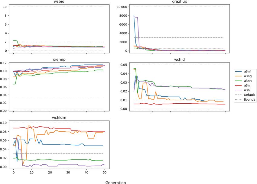
M. Falls et al.: Use of genetic algorithms for ocean model parameter optimisation                                          5719

Figure 2. An example of the Autosubmit workflow.

how the method behaves when different sizes of vectors of          3     Results
parameters are used.
   Experiment set O5_LAB1 uses the BRKGA as intended,              3.1     Default data
where the reference data are observed data from LAB1, and
the outputs are analysed. This is further compared with ex-        3.1.1    The nine parameters (D9)
periment sets O5_LAB2 and O5_LAB3, which are run in
LAB2 and LAB3, respectively. This is to investigate how the        The evolution of the optimal sets of parameters in experi-
results obtained reflect the wider region.                         ment set D9 is presented in Fig. 3. Figures 4 and 5 present
   Finally, cross-simulations are run, whereby a representa-       the cost function of each optimal set per iteration and their
tive vector of parameters from each of the experiment sets         corresponding statistics of the SPOC and LPOC. In all cases,
O5_LAB1, O5_LAB2, and O5_LAB3 is selected to run a                 most of the evolution occurs within the first 10 to 20 gener-
single simulation in the other two locations. This is to further   ations. This is evident from all figures, as the cost function
check how robust the BRKGA is and if the vectors produced          decreases rapidly towards zero, and the optimal sets of pa-
are representative of the region. In fact, a certain homogene-     rameters in all experiments initially fluctuate greatly before
ity is expected across the three locations because of their sim-   remaining at similar values for the remainder of the experi-
ilar physical and biogeochemical properties. The BRKGA             ment. The spread of the values to which the parameters tend
not capturing this homogeneity would suggest that the tool is      to converge varies strongly from one parameter to another.
compensating for other errors in the attempt to minimise the       When a parameter evolves towards its corresponding default
cost function resulting in an overfitting of the optimal vector    value in a consistent manner across the five replicate exper-
of parameters.                                                     iments, this suggests that it can be constrained from SPOC
                                                                   and LPOC variables with greater confidence and should be
                                                                   considered when trying to optimise the model against ob-
                                                                   served data. This is evident with wsbio and xremip, which
                                                                   return rapidly to the default value in most experiments. Other
                                                                   parameters, like wsbio2, wchld, wchldm, grazflux, and sol-
                                                                   goc, show larger optimisation uncertainty but converge to

https://doi.org/10.5194/gmd-15-5713-2022                                             Geosci. Model Dev., 15, 5713–5737, 2022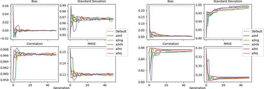
5720                                      M. Falls et al.: Use of genetic algorithms for ocean model parameter optimisation

within ±50 % of the default value in most experiments. On           BRKGA requires a larger population and a larger number of
the other hand, if the optimal values for a parameter in each       generations to be effective. However, given the difference in
of the five experiments differ from each other and the default,     the results of sets D9 and D5, there is reason to believe that
then this suggests that they cannot be constrained from POC         increasing the number of parameters in the BRKGA does not
variables in the 0–1000 m domain. This can be seen with ws-         increase the dimensionality of the problem in the way that a
bio2max and caco3r. Differences between experiments are             brute-force approach would have. Finally, increasing the vec-
also indicative of tradeoffs between parameter changes and          tor size, i.e. the number of parameters, increases the proba-
their impact on the cost function. For example, in experiment       bility of the BRKGA becoming stuck in local minima while
a274, its distinctly lower xremip value, along with its lower       searching for the optimal set.
skill of LPOC (Fig. 5), suggests that it had optimised SPOC            Experiment set D5 was additionally compared with a sim-
quickly at the expense of LPOC, causing the BRKGA to be-            ilarly structured experiment set that used a random search
come trapped in a local minimum, as indicated by the higher         algorithm to verify the better efficacy of the BRKGA. The
overall cost.                                                       results of this comparison are in Appendix C.
   The results of experiment D9, plus additional analyses
that we report in Appendix A, provided the criteria to se-          3.2     Observed data
lect the five parameters that were used in subsequent PO ex-
periments. Quite obviously, the POC sinking speed, wsbio,
and the specific remineralisation rate of both POC and GOC,         3.2.1    Labrador Sea
xremip, were selected owing to their rapid and robust con-
vergence to the expected values. In addition, wchld, wchldm,        Figure 9 shows the evolution of the optimal set of parame-
and grazflux, which showed vacillating convergence be-              ters in each generation of experiment set O5_LAB1. There
haviour in D9, were selected owing to their important role          are the following two types of behaviour observed: the pa-
in POC budgets. In particular, flux feeding (grazflux) can          rameters wchld and wchldm converge to a range that brack-
greatly attenuate the gravitational GOC flux in the upper           ets the default values, whereas wsbio, grazflux, and xremip
mesopelagic while fragmenting a fraction of GOC to POC.             clearly deviate from the default values. Still, the latter three
The parameters wchld and wchldm control detrital POC for-           parameters behave consistently across the five replicate ex-
mation through phytoplankton mortality and aggregation, es-         periments, which is in line with how they behave in D5. The
pecially during phytoplankton bloom collapse. Hence, their          parameters grazflux and xremip move beyond the extreme
inclusion is further justified by the need to optimise parame-      bounds of the initial range. This is due to the slight pertur-
ters that control POC and GOC sources and not only sinks.           bation of parameters after the crossover stage (Sect. 2.3.1).
   Figures A1 and A2 show the contribution of individual            The results also illustrate the interdependence between the
source and sink terms to the POC and GOC rates of change            parameters, such that a decrease in wsbio leads to an in-
with the default vector of parameters, demonstrating the im-        crease in certain others (see Sect. 4). The rapid evolution at
portant role of the five selected parameters. Additional ex-        the beginning is evident in the large drop in the cost func-
periments (not shown) were run with solgoc and other pa-            tion that happens during the first 10 generations (Fig. 10).
rameters not included in Table 1, supporting the choice of          As expected, the cost function is higher overall than those
the previous five parameters.                                       of the experiments against the default outputs. From Fig. 11,
                                                                    we can see that most of the statistics improve very quickly
3.1.2   The five parameters (D5)                                    at the start and that it is noticeable that the statistics for the
                                                                    LPOC are generally worse than the SPOC and hence make
The following plots analyse the results of experiment set D5.       the larger contribution to the overall ST score. Figures 12
The evolution of the optimal vector of parameters from each         and 13 are Hovmöller plots of the POC concentration profiles
generation is presented in Fig. 6. Figures 7 and 8 show the         over the annual cycle for experiment O5_LAB1 (observed,
evolution of these experiments’ statistics. When comparing          default model, and optimised model). Also included are the
these results to those of experiment set D9, an all-round im-       deviations in the default and optimised outputs with respect
provement is visible. In all cases, the parameters are more         to the observed data. With the SPOC, the improvement is
consistent and are more likely to return to the default – and       particularly noticeable in the reduction of the SPOC sinking
quicker. There is less indication of the experiments becom-         plumes in the upper mesopelagic. Whereas mean biases are
ing stuck in a local minimum, while there exists a lower cost       generally reduced, patches with positive/negative biases re-
function elsewhere within the wider space. In all cases, the        main at different times and depths after optimisation, which
cost functions are lower, and the rest of the statistics are also   is also reflected in the small improvements in correlation. It
better. Preliminary experiments where only wsbio, xremip,           must be noted that the correlation coefficients for the sim-
and grazflux were optimised (not shown) yielded even faster         ulations with default parameters were already high (0.96 for
and more robust convergence to the expected parameter val-          SPOC and 0.85 for LPOC) and thus difficult to improve. Fur-
ues. These results suggest that, with larger parameter sets, the    ther reduction in the LPOC misfit could have been impeded

Geosci. Model Dev., 15, 5713–5737, 2022                                              https://doi.org/10.5194/gmd-15-5713-2022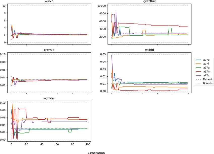
M. Falls et al.: Use of genetic algorithms for ocean model parameter optimisation                                               5721

Figure 3. Evolution of each generation’s optimal set of parameters in experiment set D9.

                                                                        by the noisier nature of the observed LPOC data (Galí et al.,
                                                                        2022).

                                                                        3.2.2   Experiments in other locations and cross-testing

                                                                        The experiments producing the median cost function for each
                                                                        set of O5_LAB1, O5_LAB2, and O5_LAB3 are presented
                                                                        in Table 3. We can see that the results are fairly consistent
                                                                        with each other, albeit some minor differences (for exam-
                                                                        ple wsbio in O5_LAB1 and grazflux in O5_LAB2), indicat-
                                                                        ing that the genetic algorithm behaves consistently from a
                                                                        regional perspective. This consistency is further confirmed
                                                                        when cross-simulations are performed on the results. These
                                                                        cross-simulations are performed by using the parameter set
                                                                        produced for one location to run single simulations at the
                                                                        other two locations. The bias and correlation of SPOC and
                                                                        LPOC between the outputs of these simulations and the re-
Figure 4. Evolution of each generation’s lowest ST score for exper-     spective observed data are calculated. These statistics, along
iment set D9.                                                           with the bias and correlation of the simulations with default
                                                                        parameters, are presented in Tables 4 (SPOC) and 5 (LPOC).
                                                                        In all cases, when a parameter set obtained from one location
                                                                        is applied to another, the outputs show reasonable consis-

https://doi.org/10.5194/gmd-15-5713-2022                                                   Geosci. Model Dev., 15, 5713–5737, 2022
5722                                       M. Falls et al.: Use of genetic algorithms for ocean model parameter optimisation

Figure 5. Evolution of each optimal generation’s bias, normalised standard deviation, correlation, and RMSE of experiment set D9.

Figure 6. Evolution of each generation’s optimal set of parameters for experiment set D5.

tency. For LPOC, all cross-tests show a substantial improve-            ing an improvement with correlation, but it is less clear. This
ment in the bias with respect to the default outputs and very           could be due to the default outputs’ biases already being very
little improvement – if any – with correlation, which is con-           low and their correlation being very high.
sistent with the outputs from the original location. There are
indications of consistency with SPOC, with nearly all show-

Geosci. Model Dev., 15, 5713–5737, 2022                                                     https://doi.org/10.5194/gmd-15-5713-2022
M. Falls et al.: Use of genetic algorithms for ocean model parameter optimisation                                                    5723

Table 3. The final parameter sets of three genetic algorithm experiments run in three locations, along with the default.

                                      Parameter      Default   Labrador 1    Labrador 2     Labrador 3
                                      wchld           0.010        0.0217         0.0392         0.0203
                                      wchldm          0.030        0.0042         0.0358         0.0757
                                      wsbio               2         0.795          0.179          0.008
                                      xremip          0.035         0.114          0.094          0.078
                                      grazflux         3000          77.3            9.8           72.2

Table 4. Comparison of SPOC absolute bias and correlation of 12 single simulations run by crossing the four parameter sets (the default
and three optimised sets produced by the BRKGA at three locations) with three locations. Values in italics mark the diagonals with equal
locations and parameter sets.

                                                                      Parameter set
                          Location               Default        Labrador 1          Labrador 2            Labrador 3
                          LAB1          0.0602, 0.958      –0.00200, 0.966    0.07737, 0.9641        0.128, 0.963
                          LAB2         −0.0194, 0.914      −0.0820, 0.931     –0.00244, 0.931       0.0506, 0.931
                          LAB3         −0.0557, 0.930       −0.127, 0.943     −0.0255, 0.929      0.00446, 0.9362

                                                                          ters selected from the initial nine-parameter vector. This par-
                                                                          ticular set of experiments produced results that were closer
                                                                          to the result of the default parameter vector with less compu-
                                                                          tation. This leads us to believe that the size of the experiment
                                                                          required is dependent on the size of the parameter vector.
                                                                          One of the main contributions of this work is to use a state-
                                                                          of-the-art ocean model as a prior step to the calculation of
                                                                          the fitness function, with all the complexity that this option
                                                                          entails. This is only possible because of the aforementioned
                                                                          availability of computing power, and it is also highly facili-
                                                                          tated by the usage of advanced scientific workflow solutions
                                                                          that allow the integration of the model executions in the evo-
                                                                          lutionary workflow (Oana and Spataru, 2016; Dueben and
                                                                          Bauer, 2018; Rueda-Bayona et al., 2020).
Figure 7. Evolution of each generation’s lowest ST score in exper-
                                                                             After the experiments against default data, the BRKGA
iment set D5.                                                             was then tested by using observed data from ocean floats in
                                                                          the North Atlantic as the reference data. A set of five experi-
                                                                          ments was run for each BGC–Argo float annual time series,
                                                                          using the same settings as in the previous set. From Fig. 9,
4   Discussion                                                            we can see that the results show a similar level of consistency
                                                                          to those with the default data. There is a visible improvement
A set of experiments was designed to test the potential of                in the outputs of the simulations that use a set of parameters
a newly developed BRKGA. As a validation, the BRKGA                       that have been optimised by the BRKGA compared to the
was first tested against the output of a simulation produced              outputs with the default parameter simulations (Figs. 12 and
with known default parameter settings. For the first set of ex-           13). However, most of the optimised parameter values tended
periments, we chose nine parameters, expressed as a vector,               rapidly towards the optimisation bounds (Table 1), and some
insuring a broad selection. This guided our choosing of pa-               even exceeded them thereafter because parameters were al-
rameters that could be constrained with confidence from the               lowed to exceed the bounds by a small percentage in each
evaluated variables (in this case, SPOC and LPOC). In ad-                 generation. This behaviour makes us question whether the
dition, in this set (and all others in the paper) five identical          optimised values are realistic, although it is also possible that
experiments were run at a time, and all results were similar              we imposed too-strict bounds in some cases, given the wide
to each other; this indicates that this method behaves consis-            range of plausible ranges that characterises some parameters
tently and reliably. The next set of experiments was identical            (see below). The problem of obtaining a right answer for the
to the previous set, except that there were only five parame-

https://doi.org/10.5194/gmd-15-5713-2022                                                      Geosci. Model Dev., 15, 5713–5737, 2022
5724 M. Falls et al.: Use of genetic algorithms for ocean model parameter optimisation Figure 8. Evolution of each generation’s optimal bias, normalised standard deviation, correlation, and RMSE in experiment set D5. Figure 9. Evolution of each generation’s optimal set of parameters for experiment set O5_LAB1. wrong reasons is common to all PO methods when applied the value of other parameters, this may indicate that a process to complex and heavily parameterised systems (Löptien and is poorly represented by the model equations. In such cases, Dietze, 2019; Kriest et al., 2020). Therefore, PO must always PO can prompt further model development. be followed by a critical evaluation of the results. If a param- Another concern that arises from the results is the need to eter converges repeatedly to unrealistic values, regardless of carefully evaluate the behaviour of the cost function. This is Geosci. Model Dev., 15, 5713–5737, 2022 https://doi.org/10.5194/gmd-15-5713-2022
M. Falls et al.: Use of genetic algorithms for ocean model parameter optimisation                                                   5725

Table 5. Comparison of LPOC absolute bias and correlation of 12 single simulations run by crossing the four parameter sets (the default
and three optimised sets produced by the BRKGA at three locations) with three locations. Values in italics mark the diagonals with equal
locations and parameter sets.

                                                                      Parameter set
                           Location          Default         Labrador 1           Labrador 2        Labrador 3
                           LAB1         0.235, 0.853    0.00172, 0.854      −0.00755, 0.830      0.0510, 0.850
                           LAB2         0.247, 0.822   −0.00710, 0.819       0.00939, 0.808      0.0574, 0.812
                           LAB3         0.194, 0.850    −0.0782, 0.854       −0.0886, 0.813     –0.0325, 0.836

                                                                         reference variables exhibit very different variability ranges
                                                                         (Friedrichs et al., 2007; Ayata et al., 2013).
                                                                            Further work quantifying the effectiveness of the cost
                                                                         functions across different situations would probably improve
                                                                         the efficacy of the BRKGA. Yet, it must be highlighted that
                                                                         the test case chosen to evaluate the BRKGA is an exigent one
                                                                         because model skill was already very good with the default
                                                                         parameters, even though PISCES was not originally tuned to
                                                                         fit these particular observations. Ongoing work with a dif-
                                                                         ferent optimisation case indicates that the BRKGA can pro-
                                                                         duce larger and simultaneous improvements in all skill met-
                                                                         rics when starting from a state of very poor model perfor-
                                                                         mance, which is, in this case, the seasonal cycle of sea sur-
                                                                         face chlorophyll a in the Tasman Sea ( Joan Llort„ personal
                                                                         communication, 2022; data not shown). Therefore, the trade-
Figure 10. Evolution of each generation’s lowest ST score of exper-
                                                                         offs between skill metrics observed here during the evolution
iment set O5_LAB1. The label of default refers to the cost function
                                                                         of the experiments may indicate that the optimisation was
of the default simulation.
                                                                         operating close to the best skill attainable with a given set of
                                                                         model equations and considering observational uncertainty.
well illustrated by Figs. 4 and 5, which show that, on occa-                As a further test of our approach, two more sets of experi-
sion, some statistics were improved at the expense of others,            ments were carried out in different locations in the Labrador
for example, bias at the expense of correlation. Correctly bal-          Sea, resulting in a reasonable consistency of the optimal pa-
ancing bias, variability, and pattern (correlation) statistics in        rameter set across the region. To confirm this, the optimal
the cost function is critical to obtain meaningful PO results.           parameter sets for the three locations were cross-referenced
Traditional cost functions based solely on the RMSE tend to              by using each parameter set in each of the other two loca-
reward solutions with too-low variability, whereby the posi-             tions in single simulations. Results from this cross-testing
tive biases cancel out the negatives (Jolliff et al., 2009, and          suggest that the parameters produced have the potential to
references therein). Cost functions such as the ST score used            be representative of the region or even exchangeable among
here (Jolliff et al., 2009) were designed to avoid this problem.         multiple locations (Table 3), meaning that the BRKGA is
However, their behaviour is also sensitive to the overall vari-          not compensating for other biases (e.g. physics) by overfit-
ability and the signal-to-noise ratio in the data. Our prelimi-          ting (Löptien and Dietze, 2019; Kriest et al., 2020). This is
nary tests suggested slightly better BRKGA performance af-               an important aspect because it means the BRKGA could be
ter the logtransformation of the data. This procedure reduced            used to investigate the large-scale spatial variability in key
the weight of the very high POC concentrations present only              biogeochemical parameters. In particular, in the past decade,
in the surface layer in spring–summer, favouring the repre-              several authors have investigated the spatial variability in the
sentation of the portions of the water column with lower                 transfer efficiency of POC from the surface ocean to its in-
POC (i.e. the mesopelagic). Unlike the model outputs used                terior using different approaches and arriving at contrasting
to test the BRKGA in the first set of experiments, the BGC–              conclusions (Henson et al., 2011; Marsay et al., 2015; Guidi
Argo POC estimates are noisy. Therefore, the cost function               et al., 2015; Weber et al., 2016; Schlitzer, 2004; Wilson et al.,
may have been less effective when faced with the observed                2015). Such spatial variability would be very difficult to es-
data. The performance of the cost function could also be im-             tablish in a three-dimensional framework because of the high
proved by applying different weights to each variable, in this           computational cost required. This is an example of the still-
case SPOC and LPOC, which is common practice when the

https://doi.org/10.5194/gmd-15-5713-2022                                                   Geosci. Model Dev., 15, 5713–5737, 2022
5726 M. Falls et al.: Use of genetic algorithms for ocean model parameter optimisation Figure 11. Evolution of each generation’s optimal bias, normalised standard deviation, correlation, and RMSE of experiment set O5_LAB1. Figure 12. The top row shows data plots of SPOC in log scale, for (left–right) observed data, the default parameter set’s model output, and the optimised parameter set’s model output. The bottom row shows the biases between the model outputs and observed data for the default parameter set (left) and optimised parameter set (right). Mean biases of the default and the optimised parameter sets are shown in Fig. 11. open scientific questions that could be tackled with our ap- Full exploitation of the results, with thousands of alternative proach. model realisations, could yield further insights on how pa- The optimisation of PISCES parameters against BGC– rameters interact in a space constrained by optimal model Argo presented in our study illustrates how PO can help us performance. understand a dynamical system better. Here we will briefly In the three O5 experiments, wsbio converged to values discuss the lessons learnt from the O5 experiments, while between 0 and 1 m d−1 . The decrease in the POC sink- keeping in mind that a detailed review of PISCES parame- ing speed improved the fit to observations by reducing the ter values and their biogeochemical implications is beyond plumes of sinking POC that formed below intense phyto- the scope of this paper. It is also noteworthy that the inter- plankton blooms in the simulations (Fig. 12). Galí et al. pretation provided here draws only from the analysis of the (2022) identified these plumes as being the main reason for best-performing parameter set in each BRKGA experiment. SPOC model–data misfit in the upper mesopelagic in sev- Geosci. Model Dev., 15, 5713–5737, 2022 https://doi.org/10.5194/gmd-15-5713-2022
M. Falls et al.: Use of genetic algorithms for ocean model parameter optimisation                                                    5727

Figure 13. The top row shows data plots of LPOC in log scale, for (left–right) observed data, the default parameter set’s model output, and
the optimised parameter set’s model output. The bottom row shows the biases between the model outputs and observed data for the default
parameter set (left) and optimised parameter set (right). Mean biases of the default and the optimised parameter sets are shown in Fig. 11.

eral subpolar locations in the Northern and Southern hemi-              uct of mesozooplankton biomass, grazflux, and particle sink-
spheres. The decrease in wsbio effectively turned the SPOC              ing speed. In PISCES, a fraction of the intercepted GOC
fraction into suspended POC, which is plausible accord-                 is fragmented into POC. Therefore, flux feeding acts to re-
ing to field studies that sorted POC fractions according to             move POC and GOC (preferentially the fast-sinking GOC)
their sinking speed (Riley et al., 2012; Baker et al., 2017).           and simultaneously produce POC; this process is becoming
The evolution of the remaining parameters acted to adjust               an important POC source in the lower mesopelagic (Figs. A1
the magnitude and shape of POC vertical profiles. Increased             and A2). Although a decrease in grazflux provided the best
xremip implies a steeper vertical decrease in both POC and              fit to observations, an increase in grazflux could also im-
GOC, with a stronger effect on POC given its much longer                prove model skill, as shown by the relatively good skill of
residence time in the mesopelagic. The xremip parameter                 experiment a3nj during the first few generations (Figs. 9 and
represents the maximal specific remineralisation rate attain-           10). This dual behaviour is confirmed by sensitivity analy-
able in the model, corresponding to freshly produced detritus,          ses (Fig. B3) which show that, for a given xremip, a de-
normalised to a temperature of 0 ◦ C with a power law tem-              crease in POC (which improves the model–data fit in the
perature dependence (Aumont et al., 2015). Our optimised                upper mesopelagic) can be achieved by either increasing or
xremip range, 0.078–0.114 d−1 , is consistent with the median           decreasing grazflux. Overall, these findings provide further
of the highest values found across six field and laboratory             evidence for the difficulty of constraining this important pa-
studies when normalised to 0◦ in the same way, i.e. 0.10 d−1            rameter (Jackson, 1993; Stemmann et al., 2004; Gehlen et al.,
(Belcher et al., 2016, and references therein), with an abso-           2006; Stukel et al., 2019).
lute maximum of 0.135 d−1 (Iversen and Ploug, 2010). De-                   The selection of a subset of model parameters is a com-
creased POC sinking speed and increased remineralisation                mon limitation of PO experiments, and although we based it
would deplete mesopelagic POC during the productive sea-                on objective criteria, we acknowledge that it remains some-
son (central panel of Fig. B1) and, hence, SPOC if they were            what arbitrary. The stepwise reduction in the number of pa-
not compensated by other processes. In our PO experiments,              rameters from nine to five obeys the need to assess the GA
this deficit was compensated by slightly increased surface              performance with a varying number of parameters and also to
microphytoplankton mortality and aggregation (wchld and                 reduce the degrees of freedom, given that only two variables
wchldm), which supply SPOC and LPOC.                                    were used as reference observations. Among the excluded
   Interpretation of the evolution of the grazflux parameter is         parameters, wsbio2 certainly deserves examination in future
more complex. The flux-feeding rate depends on the prod-                experiments, given its primary control on the fate of GOC

https://doi.org/10.5194/gmd-15-5713-2022                                                   Geosci. Model Dev., 15, 5713–5737, 2022
You can also read