Contributions of natural and anthropogenic sources to ambient ammonia in the Athabasca Oil Sands and north-western Canada
←
→
Page content transcription
If your browser does not render page correctly, please read the page content below
Atmos. Chem. Phys., 18, 2011–2034, 2018
https://doi.org/10.5194/acp-18-2011-2018
© Author(s) 2018. This work is distributed under
the Creative Commons Attribution 4.0 License.

Contributions of natural and anthropogenic sources to ambient
ammonia in the Athabasca Oil Sands and north-western Canada
Cynthia H. Whaley1,2 , Paul A. Makar1 , Mark W. Shephard1 , Leiming Zhang1 , Junhua Zhang1 , Qiong Zheng1 ,
Ayodeji Akingunola1 , Gregory R. Wentworth3,4 , Jennifer G. Murphy3 , Shailesh K. Kharol1 , and
Karen E. Cady-Pereira5
1 AirQuality Research Division, Environment and Climate Change Canada, 4905 Dufferin Street,
Toronto, Ontario, Canada
2 Climate Research Division, Environment and Climate Change Canada, 4905 Dufferin Street, Toronto, Ontario, Canada
3 Department of Chemistry, University of Toronto, 80 St George Street, Toronto, Ontario, Canada
4 Environmental Monitoring and Science Division, Alberta Environment and Parks, 9888 Jasper Ave NW,

Edmonton, Alberta, Canada
5 Atmospheric and Environmental Research, Lexington, Massachusetts, USA

Correspondence: Cynthia H. Whaley (cynthia.whaley@canada.ca)

Received: 4 July 2017 – Discussion started: 17 October 2017
Revised: 25 January 2018 – Accepted: 26 January 2018 – Published: 13 February 2018

Abstract. Atmospheric ammonia (NH3 ) is a short-lived pol-      cients relative to ground, aircraft, and satellite NH3 measure-
lutant that plays an important role in aerosol chemistry and    ments significantly.
nitrogen deposition. Dominant NH3 emissions are from agri-         By running the GEM-MACH-Bidi model in three config-
culture and forest fires, both of which are increasing glob-    urations and calculating their differences, we find that av-
ally. Even remote regions with relatively low ambient NH3       eraged over Alberta and Saskatchewan during this time pe-
concentrations, such as northern Alberta and Saskatchewan       riod an average of 23.1 % of surface NH3 came from direct
in northern Canada, may be of interest because of indus-        anthropogenic sources, 56.6 % (or 1.24 ppbv) from bidirec-
trial oil sands emissions and a sensitive ecological system.    tional flux (re-emission from plants and soils), and 20.3 %
A previous attempt to model NH3 in the region showed a          (or 0.42 ppbv) from forest fires. In the NH3 total column, an
substantial negative bias compared to satellite and aircraft    average of 19.5 % came from direct anthropogenic sources,
observations. Known missing sources of NH3 in the model         50.0 % from bidirectional flux, and 30.5 % from forest fires.
were re-emission of NH3 from plants and soils (bidirectional    The addition of bidirectional flux and fire emissions caused
flux) and forest fire emissions, but the relative impact of     the overall average net deposition of NHx across the domain
these sources on NH3 concentrations was unknown. Here we        to be increased by 24.5 %. Note that forest fires are very
have used a research version of the high-resolution air qual-   episodic and their contributions will vary significantly for
ity forecasting model, GEM-MACH, to quantify the relative       different time periods and regions.
impacts of semi-natural (bidirectional flux of NH3 and for-        This study is the first use of the bidirectional flux scheme
est fire emissions) and direct anthropogenic (oil sand oper-    in GEM-MACH, which could be generalized for other
ations, combustion of fossil fuels, and agriculture) sources    volatile or semi-volatile species. It is also the first time CrIS
on ammonia volume mixing ratios, both at the surface and        (Cross-track Infrared Sounder) satellite observations of NH3
aloft, with a focus on the Athabasca Oil Sands region during    have been used for model evaluation, and the first use of fire
a measurement-intensive campaign in the summer of 2013.         emissions in GEM-MACH at 2.5 km resolution.
The addition of fires and bidirectional flux to GEM-MACH
has improved the model bias, slope, and correlation coeffi-

Published by Copernicus Publications on behalf of the European Geosciences Union.
2012                                         C. H. Whaley et al.: Sources of atmospheric NH3 in Alberta and Saskatchewan

1   Introduction                                                    of greenhouse gases (Charpentier et al., 2009) due to min-
                                                                    ing and processing by the oil industry. While NH3 volume
Ammonia (NH3 ) is a short-lived pollutant that is receiv-           mixing ratios (VMRs) surrounding the AOSR in northern
ing global attention because of its increasing concentrations.      Alberta and Saskatchewan remain relatively low – around
Emissions of NH3 – which are in large part from agricul-            0.6 to 1.2 ppbv background (this study and Shephard et al.,
tural fertilizer, livestock (Behera et al., 2013; Environment       2015) – due to low population and lack of agriculture, the
and Climate Change Canada, 2016), and biomass burning               northern Alberta and Saskatchewan ecosystems are sensitive
(Olivier et al., 1998; Krupa, 2003) – have not been regu-           to nitrogen deposition (Clair and Percy, 2015; Wieder et al.,
lated to the same extent as other nitrogen species. NH3 is          2016a, b; Vitt, 2016; Makar et al., 2018), and the modelled
the only aerosol precursor whose global emissions are pro-          background NH3 must be correct in order to understand the
jected to rise throughout the next century (Moss et al., 2010;      relative impacts of the oil sand operations. It is important
Lamarque et al., 2010; Ciais et al., 2013).                         to understand if the AOSR facilities or other sources (e.g.,
   NH3 has an atmospheric lifetime of hours to a day (Sein-         fires, re-emissions) are causing NH3 to reach levels that cause
feld and Pandis, 1998; Aneja et al., 2001). It is a base that re-   ecosystem damage. A monitoring study from 2005 to 2008
acts in the atmosphere with sulphuric acid (H2 SO4 ) and nitric     found NH3 VMRs near Fort McMurray and Fort McKay
acid (HNO3 ) to form crystalline sulphate, nitrate salts (e.g.,     (population centers in the vicinity of the oil sand facilities)
(NH4 )2 SO4 , NH4 HSO4 , NH4 NO3 ) and aqueous ions (SO2−     4 ,   to be highly variable in space and time with a range of 1.1
HSO−         −
      4 , NO3 ) (Nenes et al., 1998; Makar et al., 2003), which     to 8.8 ppbv (where the upper end corresponds to NH3 lev-
are significant components of fine particulate matter (PM2.5 ;      els found in agricultural regions of Canada and the U.S.),
e.g., Jimenez et al., 2009; Environment Canada, 2001), thus         with NH3 concentrations 1.5–3 times higher than HNO3 con-
having health (Pope III et al., 2002; Lee et al., 2015) and cli-    centrations (Bytnerowicz et al., 2010). Hsu and Clair (2015)
mate impacts (IPCC, 2013). A large portion of NH3 is read-          also found NH3 concentrations in the AOSR to be much
ily deposited in the first 4–5 km from its source, but when in      higher than HNO3 , NO−              +
                                                                                              3 , and NH4 concentrations (by 5, 23,
fine particulate form (as NH+   4 ), its lifetime is days to sev-   and 1.8 times, respectively). Thus, NH3 may contribute the
eral weeks (Galperin and Sofiev, 1998; Park et al., 2004;           largest fraction of deposited nitrogen in the AOSR compared
Behera et al., 2013; Paulot et al., 2014), and it can be trans-     to other nitrogen species. Estimates of deposition of nitro-
ported hundreds of kilometres (Krupa, 2003; Galloway et al.,        gen compounds in the AOSR are described in Makar et al.
2008; Makar et al., 2009). Deposition of NH3 and these              (2018); however, they did not include NH3 bidirectional flux
aerosols can lead to nitrogen eutrophication and soil acidifi-      or forest fires in their model simulations.
cation (Fangmeier et al., 1994; Sutton et al., 1998; Dragosits         In a previous study by Shephard et al. (2015), it was
et al., 2002; Carfrae et al., 2004). NH3 is listed as a “criteria   found that the GEM-MACH air quality forecasting model
air contaminant” (Environment and Climate Change Canada,            (Moran et al., 2010; Moran et al., 2013; Makar et al., 2015a,
2017) in order to help address air quality issues such as smog      b; Gong et al., 2015), using a domain covering the Cana-
and acid rain.                                                      dian provinces of Alberta and Saskatchewan at 2.5 km res-
   Modelling can be used to better understand NH3 pro-              olution, under-predicted summertime tropospheric ammonia
cesses. Recent NH3 models have focused on improving bidi-           VMRs by 0.4–0.6 ppbv (which is 36–100 % depending on al-
rectional flux processes and impacts of livestock. Measure-         titude – see Fig. 16 in Shephard et al., 2015) in the AOSR
ments of NH3 bidirectional flux include those in Farquhar           when compared to the Tropospheric Emission Spectrome-
et al. (1980); Sutton et al. (1993, 1995); Asman et al. (1998);     ter (TES) satellite measurements and aircraft measurements.
and Nemitz et al. (2001), with indirect support for bidirec-        Having too much modelled NHx deposition is a cause that
tional flux also in Ellis et al. (2011). Thus, these studies        was ruled out when Makar et al. (2018) showed that GEM-
were the motivation for the recent design of parameteriza-          MACH actually underestimates NHx deposition. Underes-
tions to describe this important process (Wu et al., 2009;          timating anthropogenic and agricultural emissions was also
Wichink Kruit et al., 2010; Massad et al., 2010; Zhang et al.,      ruled out as a cause since the GEM-MACH model performs
2010; Zhu et al., 2015; Fu et al., 2015; Hansen et al., 2017).      well in southern Canada and the U.S. when compared to
Additionally, satellite observations are providing valuable in-     the U.S. Ambient Ammonia Monitoring Network (AMoN).
sight into ammonia concentrations and emissions both on re-         NH3 sources known to be missing from the GEM-MACH
gional and global scales (Beer et al., 2008; Clarisse et al.,       model were forest fire emissions and re-emission of de-
2009; Shephard et al., 2011; Shephard and Cady-Pereira,             posited NH3 from soils and plants (the latter referred to as
2015; Van Damme et al., 2014; Zhu et al., 2013).                    bidirectional flux, hereafter), which would have the greatest
   The Athabasca Oil Sands region (AOSR), located in the            impact in background areas, such as northern Alberta and
north-eastern part of the province of Alberta, Canada, is a         Saskatchewan. Therefore, these two sources were added to
large source of pollution to air (Gordon et al., 2015; Liggio       an updated version of GEM-MACH and model simulations
et al., 2016; Li et al., 2017) and ecosystems (Kelly et al.,        were repeated for a 2013 summer period (12 August to 7
2009; Kirk et al., 2014; Hsu et al., 2016), as well as a source     September 2013), during which an intensive measurement

Atmos. Chem. Phys., 18, 2011–2034, 2018                                              www.atmos-chem-phys.net/18/2011/2018/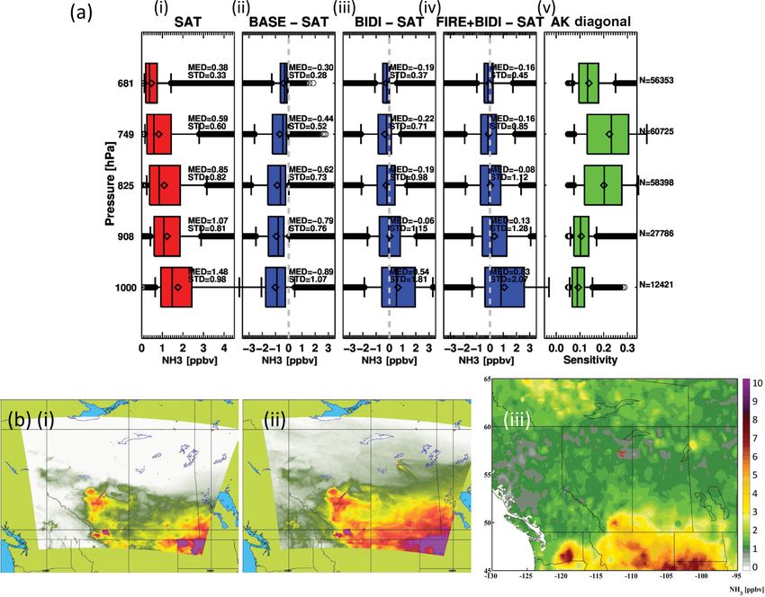
C. H. Whaley et al.: Sources of atmospheric NH3 in Alberta and Saskatchewan                                               2013

campaign occurred. We utilize ground, aircraft, and satel-        2.1   Emissions
lite measurements of NH3 and related species to evaluate the
model and to quantify the impacts of the different sources on     The emissions of 25 species (SO2 , SO4 gas, sulphate, nitrate,
atmospheric NH3 and its deposition.                               NH+ 4 , NO, NO2 , NH3 , CO, nitrous acid, benzene, propane,
   Section 2 provides the model description. Section 3 pro-       higher alkanes, higher alkenes, ethene, toluene, aromatics,
vides a brief description of ammonia measurements during          formaldehyde, aldehydes, methyl ethyl ketone, creosol, iso-
the campaign. Section 4 presents the evaluation of three          prene, crustal material, elemental carbon, and primary car-
model scenarios against three different types of measure-         bon) used in GEM-MACH (base case) come from Cana-
ments (surface, aircraft, and satellite), and Sect. 5 presents    dian and U.S. emissions inventories: the 2011 National Emis-
our quantitative assessment on the impacts of different           sions Inventory (known as NEI) version 1 for U.S. emissions
sources of NH3 to ambient VMRs and NHx fluxes in the re-          and the Air Pollutant Emission Inventory (APEI) 2013 for
gion. Our conclusions appear in Sect. 6.                          Canadian emissions (2010 for on-road and off-road emis-
                                                                  sions). Emissions were processed with SMOKE (Sparse Ma-
                                                                  trix Operator Kernel Emissions, https://www.cmascenter.org/
2   GEM-MACH model description                                    smoke/) to convert the inventories into model-ready gridded
                                                                  hourly emissions files for modelling, separated into major
GEM-MACH (Global Environment Multiscale-Modelling                 point emissions (typically industrial emissions from stacks,
Air quality and CHemistry) is an online chemical transport        emitted into the model layers that correspond to the stack
model, which is embedded in GEM, Environment and Cli-             height at the reported temperature and velocity in the inven-
mate Change Canada’s (ECCC) numerical weather predic-             tory’s stack parameters), and area emissions (emissions from
tion model (Moran et al., 2010). This means that the chemi-       spread-out sources, such as transportation and agriculture,
cal processes of the model (gas-phase chemistry, plume rise       emitted into the first model layer). For more details about
emissions distribution, vertical diffusion and surface fluxes     these emissions, see Moran et al. (2015) and Zhang et al.
of tracers, and a particle chemistry package including particle   (2018).
microphysics, cloud processes, and inorganic heterogeneous           The emissions data for NH3 from oil sand sources are
chemistry) are imbedded within GEM’s physics package,             reported to the Canadian National Pollutant Release Inven-
which in turn is imbedded within GEM’s dynamics package,          tory (NPRI) on a “total annual emissions per facility” basis.
the latter handling chemical tracer advection. A detailed de-     NH3 emissions are generally more uncertain than SO2 and
scription of the process representation of GEM-MACH, and          NOx emissions because NH3 emissions are not measured to
an evaluation of its performance for pollutants such as ozone     the same extent as those two. The oil sands represent only
and particulate matter (PM) appears in Moran et al. (2013);       1 % of total Alberta NH3 emissions, at approximately 1438 t
Makar et al. (2015a, b); and Gong et al. (2015).                  in 2013. For comparison, about 18 times more NOx and
   GEM-MACHv2 is used operationally to issue twice-daily,         57 times more SO2 was emitted from the oil sand facilities
48 h public forecasts of criteria air pollutants (ozone, nitro-   that year (http://www.ec.gc.ca/inrp-npri/donnees-data/index.
gen oxides, PM), as well as the Air Quality Health Index          cfm?lang=En). However, we found an issue with NH3 in this
(https://ec.gc.ca/cas-aqhi/). Any improvements to NH3 in the      inventory that impacted our model evaluation in the region,
model may result in better Air Quality Health Index predic-       which we describe below.
tions, since NH3 is a major precursor of PM2.5 , as mentioned        If stack parameters (e.g., stack height and diameter, vol-
in the introduction. We start with a similar research version     ume flow rates, temperatures, etc.) are included as part of
of GEM-MACHv2 (rev2285) to make the bidirectional flux            those NPRI data, then the emissions are allocated to large
modifications. The key differences between this and older         stacks in our configuration of the SMOKE emissions pro-
versions are the use of a more recent meteorological package      cessing system. In the absence of this information, SMOKE
(GEMv4.8), the capability to nest in the vertical dimension       will assign default stack parameters based on its source cat-
as well as the horizontal dimension, and improvements to the      egory code. For the Syncrude Canada Ltd. – Mildred Lake
treatment of fluxes, vertical diffusion, and advection.           plant site, NPRI ID 2274 (a facility in the AOSR), the de-
   GEM-MACH can be run for many different spatial do-             fault stack parameters were the following: 18.90 m for the
mains, at various spatial resolutions, and in 2-bin or 12-bin     stack height (which is within the first model layer), 0.24 m
aerosol-size-distribution modes. For this study, we run the       for the stack diameter, 320.0 K for the exhaust temperature,
model in the 2-bin mode (for computational efficiency), us-       and 0.58 m s−1 for the exhaust velocity. However, when these
ing a nested set of domains. The outer domain at 10 km reso-      defaults were applied to NH3 emissions in initial model sim-
lution covers North America and the inner domain at 2.5 km        ulations, they were found to result in erroneous short-term
resolution covers the provinces of Alberta and Saskatchewan.      plume events with simulated surface NH3 levels up to 2
The latter is referred to as the 2.5 km oil sands domain. This    orders of magnitude higher than ground observations, and
setup, along with the emissions described in the next section,    modelled VMRs aloft too low compared to aircraft mea-
is hereafter called our “base” simulation.                        surements. Conversely, for species such as SO2 , for which

www.atmos-chem-phys.net/18/2011/2018/                                               Atmos. Chem. Phys., 18, 2011–2034, 2018
2014                                               C. H. Whaley et al.: Sources of atmospheric NH3 in Alberta and Saskatchewan

stack parameters were reported, the model was able to cor-             the water contained in the apoplast within the leaf and in the
rectly place the SO2 enhancements in space and time, rela-             soil where NH3 (g) in the soil pore air space is in equilib-
tive to observations. When we applied those same stack pa-             rium with the NH+             −
                                                                                          4 and OH dissolved in soil water (Pleim
rameters for NH3 emissions as well (stack height = 183 m,              et al., 2013). A = 16 1500 mol K L−1 (Nemitz et al., 2000),
stack diameter = 7.9 m, exit temperature = 513 K, exit veloc-          or 2.7457 × 10¹⁵ µg K m−3 (Pleim et al., 2013) for NH3 for
ity = 23.9 m s−1 , from the NPRI website), the simulation of           both stomata and soil. B = 10 380 K (Nemitz et al., 2000).
surface NH3 was greatly improved. All subsequent simula-               0st,g is the emission potential of the stomata and ground, re-
tions reported here make use of this correction, and we advise         spectively and, in theory, is equal to the NH+4 concentration
the reporting of stack parameters for all species for future in-       over the H+ concentration in the apoplast water of the canopy
ventories in order to avoid this kind of error for models.             leaves or soil water:

2.2    Ammonia bidirectional flux parameterization                               [NH+4 ]st,g
                                                                       0st,g =      +
                                                                                             .                                    (4)
                                                                                  [H ]st,g
NH3 can be both deposited from the atmosphere to the
ground and re-emitted from soils and plants back to the atmo-          However, since there are no modelled NH+            +
                                                                                                                   4 and H apoplast
sphere. The two taken together are called bidirectional flux,          water concentrations to use, we use 0st,g from Wen et al.
since the flux of NH3 can go both up and down. The sources             (2014), which is based on long-term empirical averages. Wen
of NH3 available for re-emissions are from the accumulated             et al. (2014) gives a range of values for emission potentials
NHx in the soil and stomatal water, which can arise from               for 26 land use categories (LUCs), and we use the low end
increased deposition from anthropogenic sources, as well as            of the values in our model with the following exceptions: we
from organic nitrogen decomposition (Booth et al., 2005),              further lower the 0g for agriculture LUCs to 800, and in-
N2 -fixation (Vile et al., 2014), and natural microbial action         crease 0st of boreal forest LUCs to 3000, all of which were
(McCalley and Sparks, 2008).                                           necessary in order to achieve realistic NH3 concentrations
   The bidirectional flux scheme of Zhang et al. (2010)                (e.g., compared to reported AMoN values), while staying
was applied within the GEM-MACHv2 model, replacing the                 consistent with 0 findings from the literature.
original deposition velocity for NH3 only (deposition veloc-              This version of the model, which we call GEM-MACH-
ity of other gas species follows a scheme based on a multiple          Bidi (or just “bidi” hereafter) was quite sensitive to the se-
resistance approach and a single-layer “big leaf” approach;            lection of these emission potentials, which are themselves
Wesely, 1989; Zhang et al., 2002; Robichaud and Lin, 1991;             highly uncertain (Wen et al., 2014). GEM-MACH-Bidi uses
Robichaud, 1994). The bidirectional flux scheme is described           the exact same emissions as in the base case, described in the
in detail in Zhang et al. (2010), but we summarize it here.            previous section. However, when the sign of Ft in Eq. (1) be-
   Bidirectional exchange occurs between air–soil and air–             comes positive (that is, when Ca < Cc ), the bidirectional flux
stomata interfaces. The bidirectional flux (Ft ) equation is           acts effectively as an additional source of NH3 gas, releasing
          Ca − Cc                                                      stored NH3 until and unless the ambient concentration rises
Ft = −            ,                                             (1)
          Ra + Rb                                                      to the compensation point concentration. When the flux is
                                                                       negative, net deposition of NH3 occurs.
where Ra and Rb are the aerodynamic and quasi-laminar re-
                                                                          It is important to note that Cst,g values are exponentially
sistances, respectively. Ca is the NH3 concentration in the
                                                                       dependent on temperature (Fig. 1 shows an example of this
air, and Cc is the canopy compensation point concentration,
                                                                       relationship for the dominant LUCs in the northern part of the
given by Eq. (2).
                                                                       domain), and the higher the compensation point, the greater
                          Ca      Cst      C g                         the likelihood there will be upward flux. The lower the Cst,g ,
                        Ra +Rb   +R st
                                       + Rac +Rg
Cc =                                                          , (2)    the more likely there will be deposition. Since our simulation
       (Ra + Rb )−1 + (Rst )−1 + (Rac + Rg )−1 + (Rcut )−1
                                                                       period was August and September 2013, when the average
where Cst and Cg are the stomatal and ground compensation              temperature in the AOSR was about 18 ◦ C (http://agriculture.
points, respectively, and Ri are the resistances in s m−1 of the       alberta.ca/acis/alberta-weather-data-viewer.jsp), we expect
ground/soil (Rg ), stomata (Rst ), cuticle (Rcut ), and in-canopy      to have more NH3 re-emission than at other times of the
aerodynamic (Rac ). All resistance formulas can be found in            year. During the rest of the year (e.g., the preceding winter
Zhang et al. (2003).                                                   and spring), the compensation point would be much lower,
  Stomata (st) and ground (g) compensation points are both             greatly increasing the likelihood to have net deposition, even
calculated using Eq. (3):                                              in northern Alberta and Saskatchewan where ambient NH3
           A         −B                                                concentrations are low. Other meteorological factors affect
Cst,g =         exp(       )0st,g .                             (3)    the magnitude of bidirectional flux via the resistance terms.
          Tst,g      Tst,g
                                                                       For example, canopy compensation points have been ob-
A and B are constants derived from the equilibria constants            served to decrease with decreasing wind velocity and in-
for NH3 (g) in leaves’ stomatal cavities to NH+        −
                                              4 and OH in              creased precipitation (Flechard and Fowler, 1998; Fowler

Atmos. Chem. Phys., 18, 2011–2034, 2018                                                    www.atmos-chem-phys.net/18/2011/2018/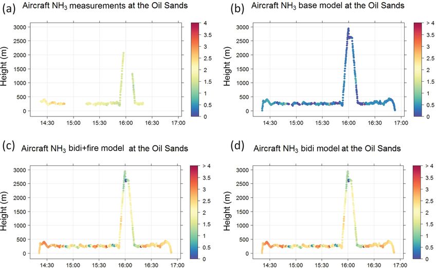
C. H. Whaley et al.: Sources of atmospheric NH3 in Alberta and Saskatchewan                                                                    2015

                                      40                                             major point emissions. The forest fire emissions system for
                                      35                                             GEM-MACH (called “FireWork is described in detail in
      Compensation point (ug m -3 )

                                      30
                                                                                     Pavlovic et al. (2016). Briefly, to calculate the fire emissions
                                                                                     for input to FireWork, biomass burning areas are first identi-
                                      25
                                                                                     fied in near-real-time by the Canadian Wildland Fire Infor-
                                      20                                             mation System (CWFIS), which is operated by the Cana-
                                      15                                             dian Forest Service (http://cwfis.cfs.nrcan.gc.ca/home). CW-
                                      10                                             FIS uses fire hotspots detected by NASA’s Moderate Res-
                                      5
                                                                                     olution Imaging Spectroradiometer (MODIS) and NOAA’s
                                                                                     Advanced Very High Resolution Radiometer and Visible In-
                                      0
                                           250   260    270      280     290   300
                                                                                     frared Imaging Radiometer Suite imagery as inputs. Daily to-
                                                       Temperature (K)               tal emissions per hotspot are then estimated by the Fire Emis-
                                                                                     sion Production Simulator module of the BlueSky modelling
Figure 1. Compensation point (Cg ) relationship to temperature; Cg                   framework (Larkin et al., 2009). SMOKE was then used to
for evergreen needleleaf LUC shown as example.                                       prepare model-ready hourly emissions of several species (in-
                                                                                     cluding NH3 ) in a point-source format for model input.
                                                                                        In ECCC’s operational forest fire forecasts, these emis-
et al., 1998; Biswas et al., 2005; Zhang et al., 2010). In other                     sions are used at 10 km resolution for the domain encompass-
words, we expect more re-emission during higher winds and                            ing North America, with forest fires being treated as point
drier conditions.                                                                    sources with specific plume rise (Pavlovic et al., 2016). We
   Other chemical transport models, such as GEOS-Chem                                have added 2013 forest fire emissions which were originally
and CMAQ, use a similar method as Zhang et al. (2010);                               created for the 2013 FireWork forecasts to the anthropogenic
however, instead of the constant average soil emission poten-                        point-source emissions used in the base case simulation, and
tials used here, they utilize a CMAQ–agroecosystem coupled                           have modified the GEM-MACH model to be able to accom-
simulation to calculate a soil pool from which to estimate 0g                        modate the changing number of major point sources each
(Bash et al., 2013; Pleim et al., 2013; Zhu et al., 2015). In this                   day (as the number of fires changes daily). Fire plume rise is
case, the emission potential will vary and can go to zero if the                     an ongoing area of investigation (e.g., Heilman et al., 2014;
NH+ 4 in the pool is depleted. However, it was shown in Wen
                                                                                     Paugam et al., 2016); smoldering emissions tend to be emit-
et al. (2014) that their 0st,g worked well during the same time                      ted directly at the surface, whereas flaming emissions can
of year as this investigation (August and September). This                           inject plumes to the upper troposphere. Here, we have set all
time of year was also shown in Zhu et al. (2015) to not have                         fire emissions to be distributed evenly throughout the bound-
a large effect on emissions from the NH+   4 pool. Additionally,
                                                                                     ary layer, which is a simplification but one that averages out
Wentworth et al. (2014) calculated the approximate relative                          smouldering and flaming plume heights. Different parame-
abundances of NHx in the boundary layer versus NH+      4 in the
                                                                                     terizations of fire plume rise are currently under development
soil pool to assess whether surface-to-air fluxes were sustain-                      in GEM-MACH. The FireWork fire emissions are described
able. They found that soil NH+    4 concentrations were much
                                                                                     in detail in Zhang et al. (2018), and this study represents the
greater than boundary layer NHx (by over 2 orders of magni-                          first time they have been used at a 2.5 km horizontal resolu-
tude), further supporting the assumption made here. In addi-                         tion.
tion, the turnover time for soil NH+ 4 is on the order of 1 day,
hence it is unlikely that NH3 bidirectional fluxes would sig-                        2.4   Model setup for three scenarios
nificantly deplete or enhance soil NH+   4 pools. Finally, given
that GEM-MACH is used for real-time air quality forecasts at                         The base, bidi, and fire + bidi models were all run in the
ECCC, it is not desirable for our bidirectional flux scheme to                       following way: each scenario was run from 1 August to 7
have to rely in advance on another model’s output. Therefore,                        September 2013, where the first 11 days were “spin up” in or-
we use this simplified version, and assess whether its results                       der to allow chemical concentrations to stabilize, and are not
provide an improvement (smaller biases and better correla-                           used in our evaluation. This is a sufficient amount of spinup
tions to measurements) to simulated NH3 .                                            time, given that the atmospheric lifetime of NH3 is typically
                                                                                     up to 1 day (Seinfeld and Pandis, 1998; Aneja et al., 2001),
2.3   Addition of forest fire emissions                                              and given that it is close to the transport time of air cross-
                                                                                     ing the larger North American domain. The time period from
Our third model scenario (called “fire + bidi” hereafter) uses                       12 August to 7 September was chosen to coincide with the
the GEM-MACH-Bidi model, and the exact same area emis-                               intensive measurement campaign described in Sect. 3.
sions and anthropogenic major point emissions as the base                               The model was run in a nested setup, whereby the North
and bidi scenarios. However, in addition, we add hourly                              American domain was run at 10 km resolution using “clima-
North American forest fire emissions for all species to the                          tological” chemical initial and boundary conditions from a 1-

www.atmos-chem-phys.net/18/2011/2018/                                                                 Atmos. Chem. Phys., 18, 2011–2034, 2018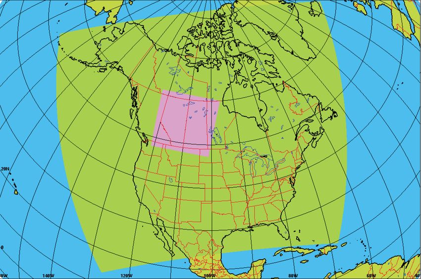
2016                                         C. H. Whaley et al.: Sources of atmospheric NH3 in Alberta and Saskatchewan

Figure 2. Map of 10 km resolution continental piloting model domain (green) and 2.5 km resolution nested model domain (purple).

year MOZART simulation for all pollutants (Giordano et al.,           3     Measurements
2015). The nested oil sands region (which covers most of
Alberta and Saskatchewan) was run at 2.5 km horizontal res-           Our three model simulations (base, bidi, and fire + bidi)
olution, using the initial and boundary conditions from the           are evaluated with surface, aircraft, and Cross-track Infrared
10 km North American model run. Figure 2 shows the two                Sounder (CrIS) satellite measurements. We briefly describe
model domains.                                                        each of these observation datasets below.
   The model simulations for the pilot and nested domains
were not run as a continuous multi-day forecast but rather            3.1    AMS13 ground measurements
following the operational air quality forecast process, where
the meteorological values are updated regularly with new              An extensive suite of instrumentation was deployed at mon-
analyses (products of meteorological data assimilation which          itoring site AMS13 (57.1492◦ N, 111.6422◦ W; 270 m a.s.l.;
provide optimized initial conditions for the 12 UTC hour of           Fig. 3) from 7 August 2013 until 12 September 2013. Min-
each day). The analyses were obtained from ECCC archives              ing operations and bitumen upgrading facilities are 5 km
(Buehner et al., 2013, 2015; Caron et al., 2015), in order to         to the south and north of the site, which is surrounded by
prevent chaotic drift of the model meteorology from obser-            boreal forest with dominant winds from the west averag-
vations. Consequently, our simulation setup comprises simu-           ing 1.9 m s−1 throughout the year. The average temperatures
lations on the North American domain in 30 h cycles starting          in the region for August are highs between 20–25 ◦ C and
at 12:00 UTC, and the oil sands domain in 24 h cycles start-          lows around 10 ◦ C, which is warm enough to make upward
ing at 18:00 UTC (the 6 h lag being required to allow mete-           NH3 flux more likely (recall Fig. 1). However, temperatures
orological spinup of the lower resolution model). The next            drop rapidly at the end of August, into September, where
cycle uses the chemical mass mixing ratios from the end of            the September highs average around 15 ◦ C and lows around
the last cycle as initial conditions for the next 24–30 h. This       5 ◦ C. The skies are the clearest during August, with at least
system of staggered meteorological driving forecasts with a           partly clear skies 50 % of the time. That said, the warm sea-
continuous chemical record continues until the full time pe-          son (May through September) is the wetter season (average
riod completes.                                                       of 20 % chance of precipitation daily), with more precipi-
   We run GEM-MACH in the 2-bin particle mode, which                  tation than during the cold season (when there is an aver-
means that particles fall in either fine mode (diameter 0–            age of 7 % chance of precipitation daily). However, year-
2.5 µm) or coarse mode (diameter 2.5–10 µm), for computa-             round precipitation, as well as relative humidity, are both rel-
tional efficiency (although sub-binning is used in some par-          atively low in the AOSR. During the cold season (November
ticle microphysics processes in order to ensure an accurate           through February), the average temperatures range from −21
representation of particle microphysics; Moran et al., 2010),         to −5 ◦ C, when the forest and soils are more likely to be a de-
and in order to follow the setup used for the operational             position sink for NH3 . During November to April, it is also
10 km resolution GEM-MACH forecast.                                   much cloudier, with February having cloudy conditions 77 %
                                                                      of the time. (All weather data cited here are from the annual

Atmos. Chem. Phys., 18, 2011–2034, 2018                                                 www.atmos-chem-phys.net/18/2011/2018/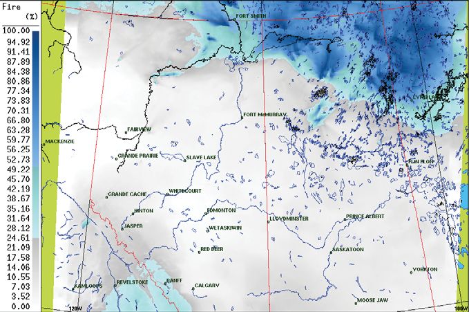
C. H. Whaley et al.: Sources of atmospheric NH3 in Alberta and Saskatchewan                                                        2017

                                                                          inlet from which the HR-ToF-AMS sub-sampled. The total
                                                                          residence time in the inlet and associated tubing was approx-
                                                                          imately 1 s. The error on these measurements is ±9 %. (Lig-
       57.4
                                                                          gio et al., 2016)
                                                                             Figure 3 shows a sample flight path from the campaign
                                                                          from 13 August 2013 – one of the 13 flights with valid NH3
                                                             Elev
       57.2                                                               measurements. The others took place on 15–17, 19 (two this
                                                                    750   day), 22–24, 26, 28 August, and 5–6 September 2013. NH3
 Lat

                                                                    500   data on the other nine flights were invalidated due to instru-
       57.0                                                         250   ment issues (those on 14, 20–21, 29, 31 August, and 2–4
                                                                          September 2013), but were successful for the NH+  4 measure-
                                                                          ments.
       56.8
                                                                          3.3    CrIS satellite measurements

               −112.0      −111.5         −111.0
                                                                          CrIS was launched in late October 2011 on board the Suomi
                                Long                                      NPP platform. CrIS follows a sun-synchronous orbit with a
                                                                          daytime overpass time at 13:30 LT (local time, ascending)
Figure 3. Flight path on 13 August 2013, where elevation (in me-
                                                                          and a night time equator overpass at 01:30 LT (descending).
tres) is denoted by the colour scale and the AMS13 site is indicated
by a black circle.
                                                                          The instrument scans along a 2200 km swath using a 3 × 3
                                                                          array of circular pixels with a diameter of 14 km at nadir for
                                                                          each pixel. The CrIS “fast physical retrieval” described by
report at Fort McMurray: https://weatherspark.com/y/2795/                 Shephard and Cady-Pereira (2015) is used to perform satel-
Average-Weather-in-Fort-McMurray-Canada-Year-Round).                      lite profile retrievals of NH3 VMR given the infrared emis-
   NH3 , fine particulate ammonium and nitrate, and other                 sion spectrum from the atmosphere. This retrieval uses an op-
species were measured by an ambient ion monitor ion chro-                 timal estimation approach (Rogers, 2000) that provides the
matograph via an inlet 4.55 m off the ground. The uncertainty             satellite vertical sensitivity (averaging kernels) and an esti-
of these measurements is ±15 %. These measurements are                    mate of the total errors (error covariance matrix).
described in more detail in Markovic et al. (2012).                          We take the CrIS retrieved profile and match it up with
   Data gaps sometimes appeared in the surface NH3 time                   the closest model profile in both distance and time, compute
series for the following reasons: instrument zero (14–15 and              the distance between the CrIS pixel and model field for each
17–18 August), instrument maintenance (19 August), and a                  time step, and then select the time step that best matches the
power outage (27–28 August).                                              satellite overpass time. Since the model time steps are every
                                                                          hour with a 10 km spatial resolution they are always matched
3.2       Aircraft measurements                                           up to better than half an hour, and within 5 km.

During the oil sands monitoring intensive campaign, there
were a total of 22 flights spanning 13 August to 7 September
2013. These measurements are described in detail in Shep-                 4     Model evaluation
hard et al. (2015); Gordon et al. (2015); Liggio et al. (2016);
and Li et al. (2017), and are summarized here. Aircraft NH3               An older version of GEM-MACH (v1.5.1) has been com-
measurements were conducted with a dual quantum cas-                      pared to TES satellite and aircraft measurements of ammo-
cade laser (QCL) trace gas monitor (Aerodyne Inc., Biller-                nia over the AOSR (Shephard et al., 2015). Simulations with
ica, MA, USA; McManus et al., 2008), collecting data ev-                  that version of the model were shown to be biased low, by
ery 1 s. Outside air was sampled through a heated Teflon in-              about −0.5 ppbv throughout the lower-tropospheric vertical
let tube shared with a high-resolution time-of-flight chemical            profile. This represented a substantial deficit in the model
ionization mass spectrometer (HR-ToF-CIMS); the flow rate                 predicted sources of NH3 , prompting the current work. We
through the QCL was 10.8 L min−1 . The 1σ uncertainty for                 now compare our three GEM-MACHv2 simulations (base,
each measurement was estimated to be ±0.3 ppbv (±35 %;                    bidi, and fire + bidi) against surface point measurements at
Shephard et al., 2015).                                                   the measurement site near an oil sands facility (AMS13),
   Particulate NH+4 (0 to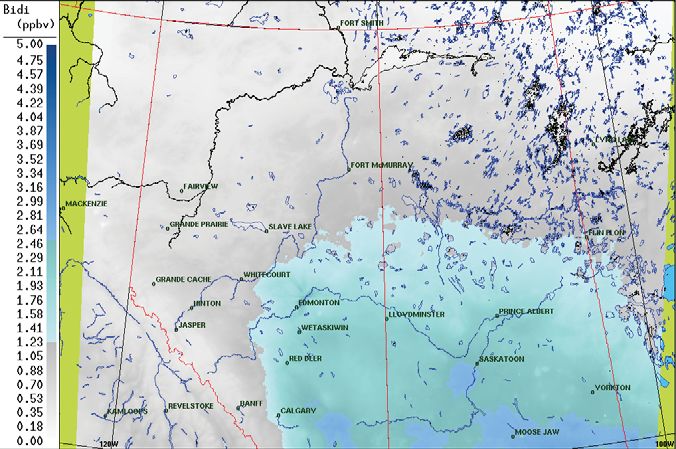
2018 C. H. Whaley et al.: Sources of atmospheric NH3 in Alberta and Saskatchewan
Surface concentrations at Oil Sands AMS13 site
Aug 12 Aug 19 Aug 26 Sep 02
(a) NH3 (ppbv) (b) NH4 (ug m-3)
3.0 − 1.0 −
−
2.5 0.8
− o
−
o − −
−
−
2.0 − −
−
−
−
−
− 0.6 o
o − o
1.5 o −
o− − − −
−
−
−
o − − − 0.4 o− − −
1.0
−
−
−
−
−
− − o −
o−
−
o − −
−
o o − o − −
−
− −
o− o o o −
− o− o −
− o o o
−
o 0.2 − − o−− −
o o−
−
0.5 o − − o o − −
− − − o−
−
o
−
o o o −
− −
− o
−
− − −
− − − − −
o o− o− o− o− o−−
− − − −
o o
− −
o −
o− − − − − − − − o−
−
− − −
− − − − − − − − − − − − o o o o o o o−
0.0 − − − − − − 0.0
(c) NO3 (ug m-3) (d) SO4 (ug m-3)
−
− −
−
−
2.5
−
0.6 o
−
2.0 o o −
−
−
0.4 − 1.5 o − −
− − − −
−
−
− − 1.0 o − −
−
o−
− −
− −
0.2 −
−
− o − −
−
o − −
− − − − −
− − − o−− o
o − −
−
o o
0.5 − o
− − − o
−
− − − −
o− o o o−− − − − o− − − −
− − −
−
−
− − − −
o o − − − − − − − o−
o− o− o−− o−−
− − − − − − −
− o− o−− o− o− o− o− o− o− o− o− o−− o−− o
− o − −
− o o o o o o o o
0.0 − −
− − − − 0.0 o o o o o o− o
Aug 12 Aug 19 Aug 26 Sep 02
o Meas − Base − Bidi − Fire
2−
Figure 4. Surface daily average VMR of (a) NH3 , and concentrations of (b) fine particulate NH+ −
4 , (c) NO3 , and (d) SO4 at the AMS13
ground site in the AOSR. Measurements (Meas) in orange, base model in green, bidirectional flux model (Bidi) in blue, and fire + bidi model
(Fire) in red.
4.1 At the AMS13 ground site Unfortunately, during some time periods, these two versions
of the model overestimate NH3 : during 13 August, the model
adds a significant level of NH3 due to fire emissions; how-
Figure 4 shows the time series of the daily average (for clar- ever, the surface in situ observations show no evidence of
ity) VMRs of NH3 and concentrations of fine-particulate fire impact. During other time periods (e.g., 30 August to 3
2−
NH+ −
4 , NO3 , and SO4 at the AMS13 oil sands ground site September, and 4–7 September), the bidi model appears to
for the observations and three model simulations. The hourly have put too much NH3 into the system. Therefore, the bidi
data were also studied, but are not shown in the time series. model bias (Fig. 5a) is now 0.30 ppbv too high (median), and
We first note that the NH3 VMRs in the measured time se- the fire + bidi bias is 0.32 ppbv high (median) over the time
ries are relatively low with mean, median, and maximum of period of the campaign, resulting in an overall improvement
0.6, 0.426, and 2.98 ppbv, respectively, in the hourly data, of only 0.03 ppbv in the model bias.
which are lower than the 1–8 ppbv range in Bytnerowicz While the bias improvement is small, the bidi and
et al. (2010) and the 2.7 ppbv summertime mean given in Hsu fire + bidi both have greatly improved correlation coeffi-
and Clair (2015). However, this may be due to the different cients (from R = 0.1 to 0.4) and slopes much closer to 1
time periods and locations measured. Our mean measured (from 0.1 to 0.7), showing that those added sources are im-
values at the AMS13 site are similar to the VMRs found portant to improve model results (Fig. 6a). Additionally, the
at U.S. AMoN background sites (http://nadp.sws.uiuc.edu/ diurnal cycle (not shown) was improved in the bidi simula-
amon/). tion, with both it and the measurements shaped like a sine
Figure 4a shows that the base model (green) background curve with a minimum at 03:00–04:00 LT, and a maximum
VMRs of NH3 are very low (nearly 0 ppbv when there is at noon local time, although the amplitude of the cycle was
no plume influence) compared to the measurements (or- underestimated. Whereas, the base model diurnal cycle was
ange). Only during the spike on 3–4 September does the base flat from midnight to noon local time, and spiky from noon
model exceed the measured values, probably indicating a lo- to midnight.
cal plume event fumigating to a lesser extent in the observa- While Figs. 4a to 6a show that the addition of bidirectional
tions than was predicted by the model. The NH3 VMRs of the flux improves the model correlation coefficient, slope, and
base case are biased low compared to the surface measure- bias, there is still room for further improvement. Paired t-
ments by a median of −0.35 ppbv (Fig. 5a) over the time pe- test results indicate that the fire + bidi and measurements are
riod of the campaign. In Fig. 4, the bidi model (blue line) and still significantly different (see Table 2 for comparison statis-
fire + bidi model (red line) show a significant improvement tics of all three simulations). While inherent limitations from
to the NH3 VMRs compared to the base model (green line).
Atmos. Chem. Phys., 18, 2011–2034, 2018 www.atmos-chem-phys.net/18/2011/2018/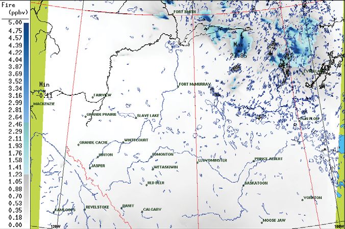
C. H. Whaley et al.: Sources of atmospheric NH3 in Alberta and Saskatchewan 2019
(a) NH3 model bias at AMS13 site (b) Fine−mode NH4 model bias
8
0.4
Med diff = 0.04 +/− 0.47 0.05 +/− 0.48 0.07 +/− 0.52
Model bias (ug m -3)
6
Model bias (ppbv)
Med diff = −0.35 +/− 0.82 0.3 +/− 0.85 0.32 +/− 0.91
4
0.0
2
−0.4
−2
Base Bidi Fire+bidi Base Bidi Fire+bidi
(c) Fine−mode NO3 model bias (d) Fine−mode SO4 model bias
0.2
Med diff = 0.23 +/− 1.7 0.16 +/− 1.68 0.21 +/− 1.73
Model bias (ug m -3 )
Model bias (ug m -3 )
Med diff = −0.01 +/− 0.31
1.0
0 +/− 0.38 0 +/− 0.45
0.0
0.0
−0.2
−1.5
Base Bidi Fire+bidi Base Bidi Fire+bidi
2−
Figure 5. Hourly model–measurement bias in surface (a) NH3 VMR, and (b) NH+ −
4 , (c) NO3 , and (d) SO4 concentrations at the AMS13
ground site in the AOSR.
(a) NH3 (b) NH4
0 1 2 3 4 5 6 7
6
Rbase= 0.103 , slope= 0.116
Rbidi = 0.413 , slope= 0.652 Rbase= 0.294 , slope= 0.346
5
Rfire+bidi= 0.403 , slope= 0.691
Model (ug m-3)
Rbidi = 0.321 , slope= 0.4
Model (ppbv)
Rfire+bidi= 0.285 , slope= 0.389
4
Base
3
Bidi
2
Fire
1
One−to−one line
0
0 1 2 3 4 5 6 7 0 1 2 3 4 5 6
Measurements (ppbv) Measurements (ug m-3 )
(c) NO3 (d) SO4
Rbase= 0.257 , slope= 0.209
6
15
Rbase= 0.121 , slope= 0.474 Rbidi = 0.254 , slope= 0.198
2 3 4 5
Rfire+bidi= 0.236 , slope= 0.194
Model (ug m-3 )
Model (ug m-3)
Rbidi = 0.277 , slope= 1.399
Rfire+bidi= 0.259 , slope= 1.518
10
5
1
0
0
0 1 2 3 4 5 6 0 5 10 15
Measurements (ug m-3) Measurements (ug m-3)
2−
Figure 6. Hourly modelled vs. measured surface (a) NH3 VMR, and (b) NH+ −
4 , (c) NO3 , and (d) SO4 concentrations at the AMS13 ground
site in the AOSR. Base model is in grey, bidirectional flux model in blue, and fire + bidi model in red.
model resolution and uncertainties may be responsible for the leaf trees, deciduous broadleaf trees, inland lake, mixed
remaining bias, it is likely that (a) the emission potentials for shrubs, and mixed forests (and none of the region to swamp).
the LUCs in the region may be causing too much re-emission This would lead to an overestimation of re-emission given
of NH3 , and need refinement, and (b) the fire emissions of that bogs are fairly acidic and our swamp emission potential
NH3 are not properly distributed in the vertical, placing too is lower than the aforementioned LUCs. Other evidence for
much NH3 near the surface and/or the fire emission factors these two explanations will be presented below in Sect. 4.3.
2−
for NH3 are too high. For NH+ −
4 , NO3 and SO4 the time series, model biases,
Refinement needed for the emission potentials and LUCs and model-vs.-measured correlations are shown in Figs. 4,
may be a significant cause of the bidi and fire + bidi model 5, and 6, respectively. There is very little change in NH+ 4
biases. Rooney et al. (2012) have shown that about 64 % of (Figs. 4b, 5b, and 6b) and SO2− 4 (Figs. 4d, 5d, and 6d) despite
the AOSR are wetlands (fens, bogs, and marshes), which the increase in NH3 that the bidirectional flux yields. The
should be mapped to the swamp LUC. However, our model bias is very small for all three model scenarios, and the corre-
currently assigns the AOSR landscape to evergreen needle- lation coefficients are all relatively poor. So while there is an
www.atmos-chem-phys.net/18/2011/2018/ Atmos. Chem. Phys., 18, 2011–2034, 2018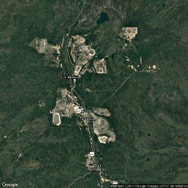
2020                                         C. H. Whaley et al.: Sources of atmospheric NH3 in Alberta and Saskatchewan

improvement to modelled NH3 with bidirectional flux, there          4.3   In the vertical profiles across the region
is a neutral affect on fine particulate NH+   4 . This may be be-
cause the charge of NH+   4 in the particles is already enough in   The CrIS satellite has many observations over North America
the base model to balance the charge of 2 × SO2−             −      during the 2013 oil sands campaign. We have evaluated the
                                                     4 + NO3 in
the aerosols, thus causing any additional NH3 (from bidi and        model with these observations in two ways:
fires) to remain in the gas phase. Alternatively, the minimal        1. All daytime data from 12 August–7 September 2013,
change in NH+   4 could be due to additional wet scavenging             with model–measurement comparisons over a large re-
of the additional NH3 , which will be discussed in Sect. 5.2.           gion encompassing Alberta and Saskatchewan (latitude
The change in NH3 VMR has no effect on SO2−          4 since par-       range: 48–60◦ N, longitude range: 100–122◦ W), which
            2−
ticulate SO4 is not sensitive to the amount of NH3 /NH+        4        contains agricultural areas, a number of cities, the north-
available, and is dominated by anthropogenic and fire emis-             ern boreal forest, and oil sand facilities.
sions. For NO− 3 (Fig. 5c), the base model bias was quite small
at 0.01 µg m−3 ; however, the addition of bidi and fire + bidi       2. Case studies where we attempt to isolate fire emissions
further reduced that bias to 0.0011 and 0.0004 µg m−3 , re-             and non-fire conditions to evaluate both new compo-
spectively, which is a significant improvement. The correla-            nents (fires and bidi) of the model.
tion coefficient for NO− 3 also improved from about 0.1 to 0.3
(Fig. 6c).                                                          The latitude and longitude ranges of our model–
                                                                    measurement pairs are given in Table 1. The satellite
                                                                    passes over these regions at approximately 13:00 LT and
4.2    Along the oil sands campaign flight paths                    01:00 LT.
                                                                       There were over 60 000 model–measurement pairs be-
There were 13 flights during the oil sands campaign that had        tween the model and the CrIS satellite over the model domain
valid (above detection limit, and no instrument error) NH3          during 12 August to 7 September 2013. Figure 9a presents
measurements, and 22 flights that had valid NH+       4 (0–1 µm     model biases for the entire dataset in a box and whiskers
diameter) measurements. The flight path of the first flight,        plot of the vertical NH3 profiles at five vertical levels. The
which occurred on 13 August 2013, is shown in Fig. 3; cho-          left-most panel (panel i) shows the NH3 VMRs measured
sen as an example because this flight sampled mainly back-          by CrIS, and the right-most panel (v) shows the diagonal
ground NH3 (rather than facility plumes).                           elements of the CrIS averaging kernels, illustrating the sen-
   Figure 7 shows the NH3 VMRs along this flight path over          sitivity of the satellite measurements to each vertical level.
time. Here the hourly model output is interpolated to the           The NH3 VMRs over Alberta and Saskatchewan measured
same time frequency as the measurements. The model output           by CrIS are very similar to those found by TES in the Shep-
also has spatial resolution limits when comparing to the air-       hard et al. (2015) study for the AOSR region.
craft. However, we clearly see that for this flight, the bidirec-      The middle panels (Fig. 9a, ii–iv) show the model biases
tional flux has increased NH3 VMRs, bringing them closer to         from the three simulations. The base model has a very simi-
the measured values (median biases for this flight are −1.38,       lar bias to CrIS as the older version of GEM-MACH (v.1.5.1)
0.68, and 0.69 ppbv in the base, bidi, and fire + bidi simu-        had compared to TES observations in the Shephard et al.
lations, respectively). There is little change when fires are       (2015) study – thus showing that the negative NH3 biases
added (Fig. 7d vs. c) because this flight did not pass through      were not improved with the use of the newer GEM-MACH
a fire plume.                                                       version (v2) itself. The fire + bidi model has the smallest bias
   Figure 8 shows the model–measurement differences and             in the highest three layers, but the bidi model has the small-
the model vs. measurement scatter plots for the combined set        est bias in the two lowest layers. In those lower layers, the
of all flight paths for hourly average NH3 and NH+   4 . For NH3    fire + bidi model increases NH3 VMRs too far (though still
the median base model bias is −0.75 ppbv, comparable to the         a smaller absolute bias compared to the base case; Fig. 9a).
bias observed in Shephard et al., 2015, with the bidi model         The fire + bidi positive bias could be due to an overestimate
bias improving to −0.24 ppbv and the fire + bidi bias im-           of the bidirectional flux re-emissions or of the fire emissions,
proving to −0.23 ppbv. Also, the best correlation coefficient       or to an underestimate of the altitude of the fire emissions,
and slope is achieved by the fire + bidi scenario. The use of       or a combination of all three factors. In order to distinguish
the bidirectional flux has thus reduced the model bias relative     between these possibilities, two case studies were examined
to the aircraft observations by a factor of 3. The fire + bidi      further in the next section. The statistics from the model–
simulation has the best statistics compared to measurements,        CrIS comparison can be found in Table 2. That summary
as summarized in Table 2.                                           shows that the fire + bidi simulation performs better than the
   Again, the NH+   4 results show little change despite the in-    base and the bidi simulations.
crease in NH3 . The small bias from the base case gets in-             The spatial distribution of modelled NH3 can also be eval-
significantly smaller, and the slope and correlation coeffi-        uated with CrIS measurements, as shown in Fig. 9b. These
cients are all negligibly changed.                                  are maps of the average surface NH3 from the base model,

Atmos. Chem. Phys., 18, 2011–2034, 2018                                              www.atmos-chem-phys.net/18/2011/2018/
C. H. Whaley et al.: Sources of atmospheric NH3 in Alberta and Saskatchewan 2021
Figure 7. NH3 VMRs aloft (colour scale) over the oil sands region during the 13 August 2013 flight. (a) Measurements, (b) base model,
(c) fire + bidi model, and (d) bidi model.
(a) NH3 model bias along flight paths (b) NH4 model bias along flight paths
0.2
Med diff = −0.751 −0.244 −0.233
1
Model bias (ug m-3)
Model bias (ppbv)
−0.2
0
−1
−0.6
−2
Med diff = −0.07 −0.065 −0.062
−1.0
Base Bidi Fire+Bidi Base Bidi Fire+Bidi
(c) Hourly average NH3 concentrations on all flight paths (d) Hourly average NH4 concentrations on all flight paths
2.0
4
Rbase= 0.368 , slope= 0.114
Rbidi = 0.549 , slope= 0.503 Rbase= 0.719 , slope= 0.364 Base
Rfire+bidi= 0.56 , slope= 0.519 Rbidi = 0.688 , slope= 0.39
1.5
Model (ug m-3)
Rfire+bidi= 0.674 , slope= 0.383 Bidi
3
Model (ppbv)
Fire
1.0
2
One−to−one line
0.5
1
0.0
0
0 1 2 3 4 0.0 0.5 1.0 1.5 2.0
Measurements (ppbv) Measurements (ug m-3)
Figure 8. Hourly averages along all flight paths over the oil sands region during the summer 2013 campaign: model–measurement bias in
(a) NH3 and (b) NH+ +
4 . Modelled vs. measured (c) NH3 VMR and (d) NH4 concentrations aloft. Base model is in grey, bidirectional flux
model in blue, and fire + bidi model in red.
the fire + bidi model, and the CrIS satellite. The fire + bidi from the spatial distribution that CrIS measures. For exam-
model over-predicts the effect of fires in the middle of north- ple, the model predicts much higher NH3 near the city of
ern Saskatchewan, but appears to be missing fires in north- Edmonton than CrIS shows. That said, the addition of bidi-
western Manitoba. Other than fire influence, the spatial dis- rectional flux has greatly improved the NH3 simulation in the
tribution in the fire + bidi model is the same as that of the northern part of the province, where it was almost zero in the
base model, but with significant increases in overall VMR. base model.
The spatial distribution of the model simulations is different
www.atmos-chem-phys.net/18/2011/2018/ Atmos. Chem. Phys., 18, 2011–2034, 20182022 C. H. Whaley et al.: Sources of atmospheric NH3 in Alberta and Saskatchewan
Table 1. Latitude and longitude ranges that the model was evaluated over with the CrIS satellite measurements.
Domain Date (in 2013) Lat. range Long. range
Alberta and Saskatchewan large domain 12 Aug to 7 Sep 48 to 60◦ N −122.0 to −100.0◦ W
Northern, no-fire case study 03 Sep 55 to 60◦ N −120.0 to −110.0◦ W
Southern, no-fire case study 01 Sep 49 to 53.5◦ N −117.0 to −106.0◦ W
Northern, fire case study 12 Aug 56.5 to 60◦ N −110.0 to −104.4◦ W
Figure 9. (a) (i) NH3 vertical profiles as measured by CrIS satellite from 12 August to 7 September 2013; difference between measurement
and (ii) base model, (iii) bidi model, and (iv) fire + bidi model; and (v) averaging kernel (labelled AK) of CrIS satellite for NH3 retrieval.
(b) Average (12 August–7 September 2013) surface NH3 VMRs given by the (i) base model, (ii) fire + bidi model, and (iii) CrIS satellite.
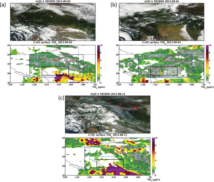
We selected three sample days (12 August and 1 and 3 we analysed for the full time period simulated (12 August–7
September 2013) that we use for the case studies. The mea- September 2013; Fig. 9a).
sured surface NH3 and sample Aqua MODIS true colour
composite maps for those days are shown (Fig. 10). The 4.3.1 Case study 1: clear-sky days with little fire
four boxed regions on those maps indicate where model– influence – evaluating bidi
measurement pairs were sampled for this study. The cyan
and black boxes (in Fig. 10a and b) are the regions where we In order to evaluate the bidirectional flux component sep-
sample clear-sky and no-fire conditions on 3 and 1 Septem- arately from the fire component, we selected 3 September
ber 2013, respectively. The magenta box in Fig. 10c is the (northern, boreal forest and AOSR region – cyan box in
region where we isolated our fire case study on 12 August Fig. 10a) and 1 September (southern, agricultural region
2013. The blue box is the region we discussed above, which – black box in Fig. 10b), where the MODIS maps (EOS-
DIS NASA Worldview map; https://worldview.earthdata.
nasa.gov/) showed very little hotspots from fires and condi-
Atmos. Chem. Phys., 18, 2011–2034, 2018 www.atmos-chem-phys.net/18/2011/2018/C. H. Whaley et al.: Sources of atmospheric NH3 in Alberta and Saskatchewan 2023
Table 2. Model–measurement NH3 comparison statistics from 12 August to 7 September 2013: R is correlation coefficient; slope is of the
line-of-best-fit between model vs. measurement; p and t are from a paired t test between model and measurement data pairs (p > 0.05 and
|t| < 1 means that the model is statistically indistinguishable from measurements); the median model bias; RMSE is the root mean square
error; and FE is the fractional error of the models. CrIS (troposphere) results are for the entire model domain at all tropospheric levels shown
in Fig. 9(top), and CrIS (surface) results are for the lowest retrieval level (both are during mid-day satellite overpass times); aircraft results
are from the 12 flight paths over the oil sand facilities, hourly averages during the daytime; and AMS13 results are from hourly data (day and
night) at the one ground station.
R Slope p t Bias (ppbv) RMSE (ppbv) FE
CrIS (troposphere)
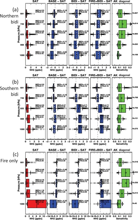
base 0.248 0.0762024 C. H. Whaley et al.: Sources of atmospheric NH3 in Alberta and Saskatchewan Figure 10. Images of the Alberta and Saskatchewan region with clouds and fire hotspots from MODIS (upper panels). Maps of CrIS-measured surface NH3 VMRs, with coloured boxes showing the regions where model and satellite measurements were sampled (lower panels). These three examples are for (a) northern bidi case study (cyan), (b) southern bidi case study (black), and (c) fire case study (magenta), discussed in Sect. 4.3, and the blue box is the region of our overall comparison. model’s oxidation rate of NO2 and SO2 in the fire may be of the Fort McMurray fires of 2016 reached only up to 3– underestimated, resulting in less sulfate and nitrate to con- 4 km altitude range based on the NASA Cloud-Aerosol Li- vert NH3 to NH+ 4 . It is potentially a combination of all three dar and Infrared Pathfinder Satellite Observation (CALIPSO) explanations, as both fire-plume rise and fire emission factors and Multi-angle Imaging Spectroradiometer (MISR) satellite are ongoing areas of study, and we further elaborate below. observations. Therefore, the fire plumes are not located above Shinozuka et al. (2011) suggest that fire plumes are the altitudes we studied. Gaussian-distributed in a thin layer aloft, which is not Unfortunately, there were no flights that captured the fine how our current fire-emissions module distributes the fire structure of the fire plumes during the 2013 monitoring in- plume. In our simulation, the fire emissions are distributed tensive campaign that can be used to further corroborate the evenly throughout the boundary layer (the first 3–4 layers vertical distribution of the fire plumes. There will, however, in Fig. 11c). However, we do not believe our parameteriza- be flight observations of fires during the planned 2018 AOSR tion of plume distribution causes the fire + bidi bias since the measurement campaign. positive bias extends throughout the first three vertical layers Explanation (b) seems the most likely, as the uncertainty and does not go negative in any layer (Fig. 11c), as would be in emission factors for NH3 from wildfires is very large (e.g., expected if mass redistribution of the plume was the cause ±50–100 % depending on the fuel type; Urbanski, 2014), of the biases. We also know that the plume heights for most and could easily be overestimated. The NOx and SO2 fire Atmos. Chem. Phys., 18, 2011–2034, 2018 www.atmos-chem-phys.net/18/2011/2018/
You can also read


