SLOW-FAST AUDITORY STREAMS FOR AUDIO RECOGNITION
←
→
Page content transcription
If your browser does not render page correctly, please read the page content below
SLOW-FAST AUDITORY STREAMS FOR AUDIO RECOGNITION
Evangelos Kazakos? Arsha Nagrani†‡ Andrew Zisserman† Dima Damen?
?
Department of Computer Science, University of Bristol
†
Visual Geometry Group, University of Oxford
ABSTRACT Slow and a Fast stream, that realise some of the properties
arXiv:2103.03516v1 [cs.SD] 5 Mar 2021
We propose a two-stream convolutional network for audio of the ventral and dorsal auditory pathways respectively. Our
recognition, that operates on time-frequency spectrogram streams are variants of residual networks and use 2D separa-
inputs. Following similar success in visual recognition, we ble convolutions that operate on frequency and time indepen-
learn Slow-Fast auditory streams with separable convolutions dently. The streams are fused in multiple representation lev-
and multi-level lateral connections. The Slow pathway has els with lateral connections from the Fast to the Slow stream,
high channel capacity while the Fast pathway operates at a and the final representation is obtained by concatenating the
fine-grained temporal resolution. We showcase the impor- global average pooled representations for action recognition.
tance of our two-stream proposal on two diverse datasets: The contributions of this paper are the following: i) we
VGG-Sound and EPIC-KITCHENS-100, and achieve state- propose a novel two-stream architecture for auditory recog-
of-the-art results on both. nition that respects evidence in neuroscience; ii) we achieve
state-of-the-art results on both EPIC-KITCHENS and VGG-
Index Terms— audio recognition, action recognition, fu- Sound; and finally iii) we showcase the importance of fusing
sion, multi-stream networks our specialised streams through an ablation analysis. Our pre-
trained models and code is available at https://github.
1. INTRODUCTION com/ekazakos/auditory-slow-fast.
Recognising objects, interactions and activities from audio is
2. RELATED WORK
distinct from prior efforts for scene audio recognition, due to
the need for recognising sound-emitting objects (e.g. alarm Single-stream architectures. A common approach in audio
clock, coffee-machine), sounds generated from interactions recognition for both scene and activity recognition, is to use
with objects (e.g. put down a glass, close drawer), and activ- a single-stream convolutional architecture [6, 7, 8]. Sound-
ities (e.g. wash, fry). This introduces challenges related to Net [8] uses 1D ConvNet trained in a teacher-student manner,
variable-length audio associated with these activities. Some and fine-tuned for acoustic scene classification. Single-stream
can be momentary (e.g. close) while others are repetitive 2D ConvNets have been extensively used by high-ranked en-
over a longer period (e.g. fry), and many exhibit intra-class tries of DCASE challenges [9, 10, 11, 12, 13, 14], for acous-
variations (e.g. cut onion vs cut cheese). Background or ir- tic scene classification. These consider spectograms as input
relevant sounds are often captured with these activities. We and utilise 2D convolutions with square k × k filters, process-
focus on two activity-based datasets, VGG-Sound [1] and ing frequency and time together [6, 7, 9, 10, 11, 12, 13, 14],
EPIC-KITCHENS [2], captured from YouTube and egocen- similarly to image ConvNets. However, symmetric filtering
tric videos respectively, and target activity recognition solely in frequency and time might not be optimal as the statistics
from the audio signal associated with these videos. of spectrograms are not homogeneous. One alternative is to
There is strong evidence in neuroscience for the existence utilise rectangular k × m filters as in [15, 16]. Another is sep-
of two streams in the human auditory system, the ventral arable convolutions with 1 × k and k × 1 filters, which have
stream for identifying sound-emitting objects and the dorsal recently been used in audio [17, 18].
streams for locating these objects. Studies [3, 4] suggest the
Multi-stream architectures. Late fusion of multiple streams
ventral stream accordingly exhibits high spectral resolution
for audio recognition was used in [19, 20, 21, 22, 23, 24, 25].
for object identification, while the dorsal stream has a high
Most approaches utilise modality-specific streams [19, 20, 21,
temporal resolution and operates at a higher sampling rate.
22]. In addition to late fusion, [20, 21] integrate multi-level
Using this evidence as the driving force for designing our
fusion in their architecture in the form of attention.
architecture, and inspired by a similar vision-based architec-
In [23, 24, 25], all streams digest the same input. In [23],
ture [5], we propose two streams for auditory recognition: a
one stream takes as input low frequencies and the second in-
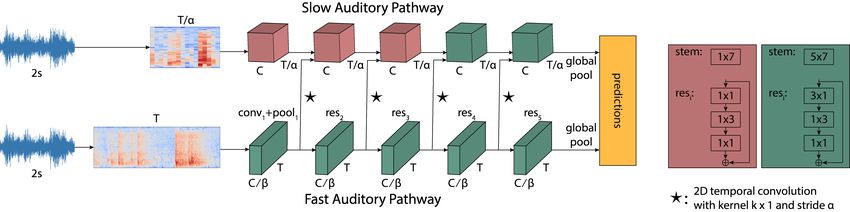
‡ Now at Google Research. puts high frequencies. [24] applies median filtering with dif-Fig. 1: Proposed Slow-Fast architecture. Strided input (by α) to the Slow pathway, along with increased channels. The Fast
pathway has less channels (by β). Right: two types of residual blocks with separable convolutions (brown vs green).
stage Slow pathway Fast pathway output sizes T ×F
ferent kernels at the input of each stream to model long dura- spectrogram - - 400×128
tion sound events, medium, and short duration impulses sep- data layer stride 4, 1 stride 1, 1
Slow : 100×128
Fast : 400×128
arately. In [25] , 1D convolutions are used with different dila- 1×7, 64 5×7, 8 Slow : 50×64
conv1
tion rates at each stream to model convolutional streams that stride 2, 2 stride 2, 2 Fast : 200×64
3×3 max 3×3 max Slow : 25×32
operate on different temporal resolutions. The architectures pool1
stride 2, 2 stride 2, 2 Fast : 100×32
of these multiple streams remain identical.
" # " #
1×1, 64 3×1, 8
Slow : 25×32
res2 1×3, 64 ×3 1×3, 8 ×3
Similar to these works, we propose to utilise two-streams Fast : 100×32
1×1, 256 1×1, 32
that consider the same input. Different from these, we design
" # " #
1×1, 128 3×1, 16
Slow : 25×16
res3 1×3, 128 ×4 1×3, 16 ×4
Fast : 100×16
each stream with varying number of channels and temporal "
1×1, 512
# "
1×1, 64
#
resolution, in addition to convolutional separation. Further- 3×1, 256 3×1, 32
Slow : 25×8
res4 1×3, 256 ×6 1×3, 32 ×6
Fast : 100×8
more, we integrate the streams through multi-level fusion. "
1×1, 1024
# "
1×1, 128
#
3×1, 512 3×1, 64
Slow : 25×4
res5 1×3, 512 ×3 1×3, 64 ×3
Fast : 100×4
1×1, 2048 1×1, 256
3. NETWORK ARCHITECTURE global average pool, concatenate, fc # classes
Next, we describe in detail the design principles of our ar- Table 1: Architecture details for Fig. 1
chitecture, depicted in Figure 1. The Slow stream operates
on a low sampling rate with high channel capacity to cap- in Fig. 1 right). By restricting the temporal resolution and
ture frequency semantics, while the Fast stream operates on a the temporal kernels of the Slow stream while keeping a high
high sampling rate with more temporal convolutions and less channel capacity, this stream can focus on learning frequency
channels to capture temporal patterns. semantics.
Input. Both streams operate on the same audio length, from The Fast stream on the other hand uses no temporal strid-
which a log-mel-spectrogram is extracted. The Fast stream ing in the input. Therefore, the intermediate feature maps
takes as input the whole log-mel-spectrogram without any have a higher temporal resolution, with temporal convolutions
striding, while the Slow stream uses a temporal stride of α throughout the stream. With a high temporal resolution and
on the input log-mel-spectrogram, where a ≥ 1. more temporal kernels while having less channels, it is easier
Slow and Fast streams. The two streams are variants of for the Fast stream to focus on learning temporal patterns.
ResNet50 [26]. Each stream is comprised of an initial con- Separable convolutions. We use separable convolutions in
volutional block with a pooling layer followed by 4 residual frequency and time as can be seen in the green block in Fig. 1
stages, where each stage contains multiple residual blocks. right. We break a 3 × 3 kernel in two kernels, 3 × 1 followed
The two streams differ in their ability to capture frequency se- by 1×3. Separable convolutions have proven useful for video
mantics and temporal patterns. The details of each stream in- recognition [27]. We utilise them with the motivation to sep-
cluding the number of blocks per stage and numbers of chan- arately attend to time and frequency of the input signal. We
nels can be seen in Table 1. contrast separable convolutions to two-dimensional filters that
The Slow stream has a high channel capacity, with β times convolve across both frequency and time.
more channels than the Fast stream, while operating on a low Multi-level fusion. Following the approach in [5], we fuse
sampling rate. As the input spectrogram is strided temporally the information from the Fast to the Slow stream with lateral
by α, the intermediate feature maps have a lower temporal connections, at multiple levels. We first apply a 2D temporal
resolution. Moreover, the Slow stream has temporal convo- convolution with a kernel 7 × 1 and a stride of α to the output
lutions only in res4 and res5 (see the brown and green blocks of the Fast stream to match the Slow stream sampling rate,and then we concatenate the downsampled feature map with Actions are mainly short-term (average action length is 2.6s
the Slow stream feature map. Fusion is applied after pool1 with minimum length 0.25s). Audio is sampled at 24kHz.
and each residual stage.
The final representation fed to the classifier is obtained
by applying time-frequency global average pooling after the 4.2. Experimental protocol
last convolutional layer of both Slow and Fast streams and
Feature extraction. We extract log-mel-spectrograms with
concantenating the pooled representations. We set α = 4 and
128 Mel bands using the Librosa library. For VGG-Sound,
β = 8 in all our experiments.
we use 5.12s of audio with a window of 20ms and a hop of
Differences compared to visual Slow-Fast [5]. Our two-
10ms, resulting in spectrograms of size 512 × 128. For EPIC-
stream architecture is inspired by its visual counterpart [5]
KITCHENS-100, we use 2s of audio with a 10ms window
which produces state of the art results for visual action recog-
and a 5ms hop, resulting in spectrograms of size 400 × 128.
nition. However, key differences are introduced: Our input
For clips < 2s in EPIC-KITCHENS-100, we duplicate the last
is 2D rather than 3D, as we operate on time-frequency while
time-frame of the log-mel-spectrogram.
the visual Slow-Fast operates on time-space. Hence, we use
2D separable convolutions decomposed as 3 × 1 and 1 × 3 Train / Val details. All models are trained using SGD with
filters, whereas [5] uses 3D separable convolutions decom- momentum set to 0.9 and cross-entropy loss. We train on
posed as 3 × 1 × 1 and 1 × 3 × 3 filters. Additionally, the EPIC-KITCHENS-100 as a multitask learning problem, as
sampling rate for audio is naturally significantly higher than in [2], using two prediction heads, one for verbs and one for
that of video, e.g. 24kHz vs 50fps in EPIC-KITCHENS-100, nouns. We train on VGG-Sound from random initialisation
and the dimensionality in video is significantly higher. Ac- for 50 epochs and fine-tune on EPIC-KITCHENS-100 using
cordingly, the approach in [5] only considers a few temporal the VGG-Sound pretrained models for 30 epochs. We drop
samples (8 and 32 frames in the Slow and Fast streams respec- the learning rate by 0.1 at epochs 30 and 40 for VGG-Sound,
tively). In contrast, our audio spectogram (see Sec 4.2) con- and at epochs 20 and 25 for EPIC-KITCHENS-100. For fine-
tains 100 and 400 temporal dimensions in the Slow and Fast tuning, we freeze Batch-Normalisation layers except the first
streams respectively. To compensate for the high sampling one, as done in [28]. For regularisation, we use dropout on
rate of audio, we temporally downsample the representations the concatenation of Slow and Fast streams with probability
of both streams by a factor of 4, using a temporal stride=2 in 0.5, plus weight decay in all trainable layers using the value
conv1 and pool1 of both streams. The remaining stages do not of 10−4 . For data augmentation during training, we use the
perform any temporal downsampling1 . implementation of SpecAugment [29] from [30] and set its
parameters as follows: 2 frequency masks with F=27, 2 time
masks with T=25, and time warp with W=5. During training
4. EXPERIMENTS we randomly extract one audio segment from each clip. Dur-
ing testing we average the predictions of 2 equally distanced
4.1. Datasets segments for VGG-Sound, and 10 for EPIC-KITCHENS-100.
VGG-Sound. VGG-Sound [1] is a large-scale audio dataset Evaluation metrics. For VGG-Sound, we follow the evalu-
obtained from YouTube. It contains over 200k clips of 10s ation protocol of [1, 7] and report mAP, AUC, and d-prime,
for 309 classes capturing human actions, sound-emitting ob- as defined in [7]. Additionally we report top-1/5% accuracy.
jects as well as interactions. These are visually-grounded For EPIC-KITCHENS-100, we follow the evaluation proto-
where sound emitting objects are visible in the corresponding col of [2] and report top-1 and top-5 % accuracy for the val-
video clip, utilising image classifiers to find correspondence idation and test sets separately, as well as for the subset of
between sound and image labels. Audio is sampled at 16kHz. unseen participants within val/test.
EPIC-KITCHENS-100. EPIC-KITCHENS-100 [2] is the Baselines and ablation study. We compare to published
largest egocentric audio-visual dataset, containing unscripted state-of-the-art results in each dataset. For VGG-Sound, we
daily activities in kitchen environments. The data are recorded also compare against [23] using their publicly available code,
in 45 different kitchens. It contains 100 hours of data, split which is the closest work to ours in motivation, as it uses two
across 700 untrimmed videos, and 90K trimmed action clips. audio streams separating input into low/high frequencies.
These capture hand-object interactions as well as activities, We also perform an ablation study investigating the im-
formed as the combination of a verb and a noun (e.g. “cut portance of the two streams as follows:
onion” and “wash plate”), where there are 97 verb classes, • Slow, Fast: We compare to each single stream individually.
300 noun classes, and 4025 action classes (many verbs and • Enriched Slow stream: We combine two Slow streams with
nouns do not co-occur). The classes are highly unbalanced. late fusion of predictions, as well as a deeper Slow stream
1 In preliminary experiments, we tried different downsampling schemes, (ResNet101 instead of ResNet50).
such as strided convolutions throughout the whole network but they resulted • Slow-Fast without multi-level fusion: Streams are fused by
in inferior performance. averaging their predictions, without lateral connections.Overall Unseen Participants
Top-1 Accuracy (%) Top-5 Accuracy (%) Top-1 Accuracy (%)
Split Model Verb Noun Action Verb Noun Action Verb Noun Action # Param.
Damen et al. [2] 42.63 22.35 14.48 75.84 44.60 28.23 35.40 16.34 9.20 10.67M
Slow 41.17 18.64 11.37 77.52 42.34 24.20 34.93 14.65 7.79 24.89M
Fast 39.84 17.07 8.76 76.94 41.31 22.01 33.33 15.21 6.57 00.49M
Val
Two Slow Streams 41.41 19.06 11.41 77.87 43.05 24.73 34.37 14.27 6.85 49.78M
Slow ResNet101 42.24 19.35 12.12 78.14 42.83 25.30 37.37 13.90 7.61 46.11M
Slow-Fast (late fusion) 42.28 19.23 11.27 78.40 44.17 25.36 34.65 15.68 7.70 25.38M
Slow-Fast (Proposed) 46.05 22.95 15.22 80.01 47.98 30.24 37.56 16.34 8.83 26.88M
Test
Damen et al. [2] 42.12 21.51 14.76 75.06 41.12 25.86 37.45 17.74 11.63 10.67M
Slow-Fast (Proposed) 46.47 22.77 15.44 78.30 44.91 28.56 42.48 20.12 12.92 26.88M
Table 2: Results on EPIC-KITCHENS-100. We provide an ablation study over the Val set, as well as report results on the Test
set showing improvement over the published state-of-the-art in audio recognition. # Parameters per model is also shown.
Model Top-1 Top-5 mAP AUC d-prime VGG-Sound. We report results in Table 3 comparing to state-
Chen et al. [1] 51.00 76.40 0.532 0.973 2.735 of-the-art from [12], which uses a single-stream ResNet50 ar-
McDonnell & Gao [23] 39.74 71.65 0.403 0.963 2.532 chitecture, [23] which uses a ResNet variant with 19 layers as
Slow 45.20 72.53 0.472 0.967 2.607 backbone for their two-stream architecture with significantly
Fast 41.44 70.68 0.442 0.966 2.576 less parameters than our model at 3.2M parameters, as well
Two Slow Streams 45.80 72.78 0.482 0.969 2.633 as ablations of our model. We report the best performing
Slow ResNet101 45.60 72.27 0.476 0.968 2.615
model on the test set in each case. Our proposed Slow-Fast
Slow-Fast (late fusion) 46.75 73.90 0.498 0.971 2.671
Slow-Fast (Proposed) 52.46 78.12 0.544 0.974 2.761 architecture outperforms [1] and [23]. The rest of our ob-
servations on the ablations from EPIC-KITCHENS-100 hold
Table 3: Results on VGG-Sound. We compare to published for VGG-Sound as well, with a key difference: the gap in
results and show ablations. performance between single streams and our proposed two-
stream architecture is even bigger for VGG-Sound, indicating
4.3. Results more complementary information in the two streams. The fact
that Slow-Fast outperforms Slow by such a large accuracy gap
EPIC-KITCHENS-100 Our proposed network achieves with an insignificant increase in parameters indicates the effi-
state-of-the-art results as can be seen in Table 2 for both cient interaction between Slow and Fast streams.
Val and Test. Our previous results [2] use a TSN with BN-
Inception architecture [28], initialised from ImageNet, while
here we utilise pre-training from VGG-Sound. Our proposed 5. CONCLUSION
architecture outperforms [2] by a good margin. We report
the ablation comparison using the published Val split. The We propose a two-stream architecture for audio recognition,
significant improvement in our proposed Slow-Fast architec- inspired by the two pathways in the human auditory system,
ture when compared to Slow and Fast streams independently fusing Slow and Fast streams with multi-level lateral connec-
shows that there is complementary information in the two tions. We showcase the importance of our fusion architec-
streams that benefit audio recognition. The Slow stream per- ture through ablations on two activity-based datasets, EPIC-
forms better than Fast, due to the increased number of chan- KITCHENS-100 and VGG-Sound, achieving state-of-the-art
nels. When comparing to the enriched Slow architectures performance. For future work, we will explore learning the
(see the last column of Table 2 for number of parameters), stride parameter and assessing the impact of the number of
our proposed model still significantly outperforms these base- channels. We hope that this work will pave the path for effi-
lines, showcasing the need for the two different pathways. We cient multi-stream training in audio.
conclude that the synergy of Slow and Fast streams is more Acknowledgements. Publicly-available datasets were used
important than simply increasing the number of parameters for this work. Kazakos is supported by EPSRC DTP, Damen
of the stronger Slow stream. Finally, our proposed archi- by EPSRC Fellowship UMPIRE (EP/T004991/1) and Na-
tecture consistently outperforms late fusion, indicating the grani by Google PhD fellowship. Research is also supported
importance of multi-level fusion with lateral connections. by Seebibyte (EP/M013774/1).6. REFERENCES classification using multi-scale features,” Tech. Rep.,
DCASE2018 Challenge, 2018.
[1] H. Chen, W. Xie, A. Vedaldi, and A. Zisserman, “VG- [15] J. Pons, O. Slizovskaia, R. Gong, E. Gómez, and
Gsound: A Large-Scale Audio-Visual Dataset,” in X. Serra, “Timbre analysis of music audio signals with
ICASSP, 2020. convolutional neural networks,” in EUSIPCO, 2017, pp.
[2] D. Damen, H. Doughty, G. M. Farinella, , A. Furnari, 2744–2748.
J. Ma, E. Kazakos, D. Moltisanti, J. Munro, T. Perrett, [16] M. Huzaifah, “Comparison of time-frequency repre-
W. Price, and M Wray, “Rescaling egocentric vision,” sentations for environmental sound classification us-
CoRR, vol. abs/2006.13256, 2020. ing convolutional neural networks,” CoRR, vol.
[3] R. Santoro, M. Moerel, F. D. Martino, R. Goebel, abs/1706.07156, 2017.
K. Ugurbil, E. Yacoub, and E. Formisano, “Encoding [17] Fanyi Xiao, Yong Jae Lee, Kristen Grauman, Jitendra
of natural sounds at multiple spectral and temporal res- Malik, and Christoph Feichtenhofer, “Audiovisual slow-
olutions in the human auditory cortex,” PLOS Compu- fast networks for video recognition,” 2020.
tational Biology, vol. 10, no. 1, pp. 1–14, 2014. [18] Z. Zhang, Y. Wang, C. Gan, J. Wu, J. B. Tenenbaum,
[4] I. Zulfiqar, M. Moerel, and E. Formisano, “Spectro- A. Torralba, and W. T. Freeman, “Deep audio pri-
temporal processing in a two-stream computational ors emerge from harmonic convolutional networks,” in
model of auditory cortex,” Frontiers in Computational ICLR, 2020.
Neuroscience, vol. 13, pp. 95, 2020. [19] Y. Su, K. Zhang, J. Wang, and K. Madani, “Environment
[5] C. Feichtenhofer, H. Fan, J. Malik, and K. He, “Slowfast sound classification using a two-stream CNN based on
networks for video recognition,” in ICCV, 2019. decision-level fusion,” Sensors, 2019.
[6] J. Salamon and J. P. Bello, “Deep convolutional neu- [20] X. Li, V. Chebiyyam, and K. Kirchhoff, “Multi-Stream
ral networks and data augmentation for environmental Network with Temporal Attention for Environmental
sound classification,” IEEE Signal Processing Letters, Sound Classification,” in Interspeech 2019, 2019.
vol. 24, no. 3, pp. 279–283, 2017. [21] G. Bhatt, A. Gupta, A. Arora, and B. Raman, “Acoustic
[7] S. Hershey, S. Chaudhuri, D. P. W. Ellis, J. F. Gem- features fusion using attentive multi-channel deep archi-
meke, A. Jansen, R. C. Moore, M. Plakal, D. Platt, tecture ,” in CHiME 2018 Workshop on Speech Process-
R. A. Saurous, B. Seybold, M. Slaney, R. J. Weiss, and ing in Everyday Environments, 2018.
K. Wilson, “Cnn architectures for large-scale audio clas- [22] H. Wang, D. Chong, and Y. Zou, “Acoustic scene clas-
sification,” in ICASSP, 2017. sification with multiple decision schemes,” Tech. Rep.,
[8] Y. Aytar, C. Vondrick, and A. Torralba, “Soundnet: DCASE2020 Challenge, June 2020.
Learning sound representations from unlabeled video,” [23] M. McDonnell and W. Gao, “Acoustic scene classifi-
in NIPS. 2016. cation using deep residual networks with late fusion of
[9] S. Suh, S. Park, Y. Jeong, and T. Lee, “Designing separated high and low frequency paths,” in ICASSP,
acoustic scene classification models with CNN vari- 2020.
ants,” Tech. Rep., DCASE2020 Challenge, 2020. [24] Y. Wu and T. Lee, “Time-frequency feature decomposi-
[10] H. Hu, C. H. Yang, X. Xia, X. Bai, X. Tang, Y. Wang, tion based on sound duration for acoustic scene classifi-
S. Niu, L. Chai, J. Li, H. Zhu, F. Bao, Y. Zhao, S. M. cation,” in ICASSP, 2020.
Siniscalchi, Y. Wang, J. Du, and C. Lee, “Device- [25] K. J. Han, R. Prieto, and T. Ma, “State-of-the-art speech
robust acoustic scene classification based on two-stage recognition using multi-stream self-attention with di-
categorization and data augmentation,” Tech. Rep., lated 1d convolutions,” in ASRU, 2019, pp. 54–61.
DCASE2020 Challenge, 2020. [26] K. He, X. Zhang, S. Ren, and J. Sun, “Deep residual
[11] K. Koutini, H. Eghbal-zadeh, M. Dorfer, and G. Wid- learning for image recognition,” in CVPR, 2016.
mer, “The receptive field as a regularizer in deep con- [27] D. Tran, H. Wang, L. Torresani, J. Ray, Y. LeCun, and
volutional neural networks for acoustic scene classifica- M. Paluri, “A closer look at spatiotemporal convolutions
tion,” in EUSIPCO, 2019. for action recognition,” in CVPR, 2018.
[12] H. Chen, Z. Liu, Z. Liu, P. Zhang, and Y. Yan, “In- [28] L. Wang, Y. Xiong, Z. Wang, Y. Qiao, D. Lin, X. Tang,
tegrating the data augmentation scheme with various and L. V. Gool, “Temporal segment networks: Towards
classifiers for acoustic scene modeling,” Tech. Rep., good practices for deep action recognition,” in ECCV,
DCASE2019 Challenge, 2019. 2016.
[13] M. Dorfer, B. Lehner, H. Eghbal-zadeh, H. Christop, [29] D. S. Park, W. Chan, Y. Zhang, C.-C. Chiu, B. Zoph,
P. Fabian, and W. Gerhard, “Acoustic scene classifi- E. D. Cubuk, and Q. V. Le, “SpecAugment: A Sim-
cation with fully convolutional neural networks and I- ple Data Augmentation Method for Automatic Speech
vectors,” Tech. Rep., DCASE2018 Challenge, 2018. Recognition,” in Interspeech, 2019.
[14] Y. Liping, C. Xinxing, and T. Lianjie, “Acoustic scene [30] “SpecAugment,” https://github.com/zcaceres/spec augment.Appendix Model Top-1 Top-5 mAP AUC d-prime
Chen et al. [1] 51.00 76.40 0.532 0.973 2.735
In this additional material, we provide further insight into ResNet50 52.23 78.08 0.542 0.974 2.747
what each of the Slow and Fast streams learn, through class ResNet50-separable 52.38 77.81 0.544 0.975 2.777
analysis and visualising feature maps from each stream. We Slow-Fast (Proposed) 52.46 78.12 0.544 0.974 2.761
also offer an ablation on separable convolutions. Finally, we
detail the hyperparameters used to train [23] on VGG-Sound. Table 4: Ablation of separable convolutions on VGG-Sound.
A. CLASS PERFORMANCE OF TWO STREAMS
on the vibraphone, while Slow extracts frequency patterns
In Figure 2, we distinguish between VGG-Sound classes that do not seem to be useful for discriminating these classes
that are better predicted from the Slow stream to the left, that contain temporally localised sounds. For sea waves
and classes that are better predicted from the Fast stream and mosquito buzzing, Slow extracts frequency patterns over
to the right. To obtain these, we calculated per-class accu- time, while Fast aims to temporally localise events, which
racy and retrieved classes for which the accuracy difference does not assist the discrimination of these classes.
is above a threshold. Particularly, we used accuracySlow −
accuracyFast > 20% to retrieve classes best predicted from C. ABLATION OF SEPARABLE CONVOLUTIONS
Slow and accuracyFast − accuracySlow > 10% to retrieve
classes best predicted from Fast. We used a higher threshold We provide an ablation of separable convolutions in Table 4.
for the Slow stream as it more frequently outperforms the We trained the ResNet50 architecture as proposed in [26]
Fast stream, as shown in our earlier results. without separable convolutions, as well as a variant with sep-
As can be seen in Figure 2, Slow predicts better animals arable convolutions. We compare this to the published results
and scenes. This matches our intuition that Slow focuses on by Chen et al. [1] that also uses a ResNet50 architecture.
learning frequency patterns as different animals make distinct Our reproduced results already outperform [1]. ResNet50-
sounds at different frequencies, e.g. mosquito buzzing vs separable has separable convolutions as used in our Slow-Fast
whale calling, requiring a network with fine spectral resolu- network (see Figure 1 and Table 1).
tion to distinguish between those. In Scenes, there are classes Results show that ResNet50-separable achieves slightly
such as sea waves, airplane and wind chime, that contain slow better results than ResNet50 in all metrics except Top-5.
evolving sounds. Although accuracy is not significantly increased in this ab-
The Fast stream, in contrast, can better predict classes lation, we employ separable convolutions in our proposed
with percussive sounds like playing drum kit, tap dancing, architecture, following our motivation to attend differently
woodpecker pecking tree, and popping popcorn. This also to frequency and time. These results also show that a single
matches our design motivation that the Fast stream learns bet- stream ResNet50 has comparable performance to our two
ter temporal patterns as these classes contain temporally lo- stream proposal, however ours performs better in accuracy
calised sounds that require a model with fine temporal reso- and the two streams accommodate different characteristics of
lution. Interestingly, Fast is better at human speech, laughter, audio classes as shown previously.
singing, and other human voices, where we speculate that it
can better capture articulation. D. HYPERPARAMETER DETAILS
Training the publicly available code of McDonnell & Gao
B. VISUALISING FEATURE MAPS
[23] with the default hyperparameters on VGG-Sound pro-
We show examples of feature maps from Slow and Fast vided poor results. We tuned the hyperparameters as fol-
streams, when trained independently (Fig 3). In each case, lows: We set the maximum learning rate to 0.01, train the
we show two samples from classes that are better predicted network for 62 epochs, with alpha = 0.1 for mixup. Lastly,
from the corresponding stream. For Slow, these are sea waves we adjusted the number of FFT points to 682 for log-mel-
and mosquito buzzing, compared to woodpecker pecking spectrogram extraction, to apply a window and hop length
tree and playing vibraphone for Fast. In each case, we show similar to the ones in [23] (their datasets are sampled at 48kHz
the input spectogram as well as feature maps from residual and 44.1kHz, while VGG-Sound is sampled at 16kHz).
stages 3 and 5. In each plot, the horizontal axis represents
time while the vertical axis corresponds to frequency. We
visualise a single channel from each feature map, manually
chosen.
In Figure 3, we demonstrate that Fast is capable of detect-
ing the hits of the woodpecker on the tree as well as the hitsFig. 2: Classes from VGG-Sound that are better predicted from Slow (left) versus Fast (right) streams. Fig. 3: Feature maps from classes that are better predicted from Slow (left) and Fast (right) streams.
You can also read