BALANCING DOMAIN EXPERTS FOR LONG-TAILED CAMERA-TRAP RECOGNITION
←
→
Page content transcription
If your browser does not render page correctly, please read the page content below
BALANCING DOMAIN EXPERTS FOR LONG-TAILED CAMERA-TRAP RECOGNITION
Byeongjun Park, Jeongsoo Kim, Seungju Cho, Heeseon Kim, Changick Kim
School of Electrical Engineering, KAIST, Daejeon, Republic of Korea
{pbj3810, jngsoo711, joyga, hskim98, changick}@kaist.ac.kr
ABSTRACT
arXiv:2202.07215v2 [cs.CV] 16 Feb 2022
Label distributions in camera-trap images are highly imbal-
anced and long-tailed, resulting in neural networks tending
to be biased towards head-classes that appear frequently. Al-
though long-tail learning has been extremely explored to ad-
dress data imbalances, few studies have been conducted to
consider camera-trap characteristics, such as multi-domain
and multi-frame setup. Here, we propose a unified frame-
work and introduce two datasets for long-tailed camera-trap
recognition. We first design domain experts, where each ex-
pert learns to balance imperfect decision boundaries caused
by data imbalances and complement each other to generate
domain-balanced decision boundaries. Also, we propose a
flow consistency loss to focus on moving objects, expecting
class activation maps of multi-frame matches the flow with
optical flow maps for input images. Moreover, two long-tailed
camera-trap datasets, WCS-LT and DMZ-LT, are introduced
to validate our methods. Experimental results show the effec-
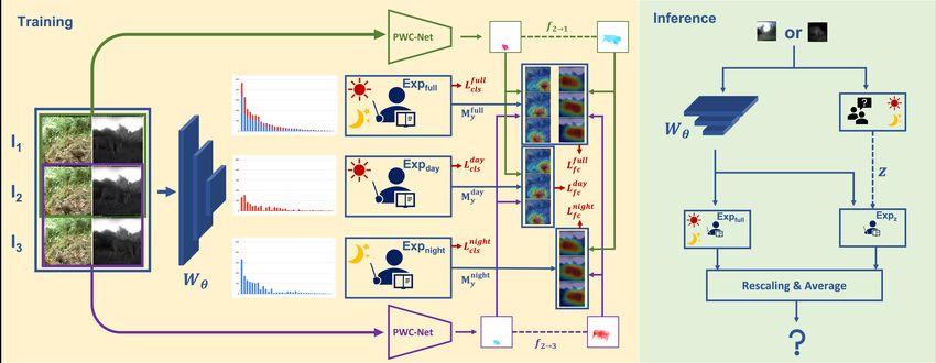
Fig. 1. Two classes are highly imbalanced between two do-
tiveness of our framework, and proposed methods outperform
mains. Existing long-tailed recognition methods resolve the
previous methods on recessive domain samples.
imbalanced label distribution (black dotted line). However,
Index Terms— Long-tailed recognition, Multi-domain the discriminability of recessive domain features is not suffi-
and multi-frame camera-trap dataset, Flow consistency ciently improved due to data imbalances, resulting in samples
being located near the boundary. Consequently, IR bound-
1. INTRODUCTION aries (blue dotted line) and RGB boundaries (RGB dotted
line) are still biased towards the head-class of each domain.
Biologists and ethologists often use camera-traps to cap- Thus, we propose that domain experts balanced by a simple
ture animals inconspicuously to study the population biol- re-weighting method give a margin for tail-classes of each do-
ogy and dynamics [1]. While these cameras automatically main, and experts complement each other to generate domain-
collect massive data, identifying species by humans is time- balanced decision boundaries (blue-black-red solid line).
consuming and labor-intensive, limiting research productiv-
ity. Therefore, deep neural networks [2, 3] have recently re- recognition by forcing experts to learn each classifier for dif-
ceived attention for their ability to automate the identification ferent sub-groups in parallel [10, 11].
process, making camera-trap studies scalable [4, 5]. Never- Despite these efforts to prefer tail-classes, limited efforts
theless, neural networks tend to be biased towards the species have been made to address the data imbalance between do-
that frequently appear, limiting studies that require diverse an- mains when images are acquired from multiple domains with
imal species, specifically on endangered species. different label distributions. Especially in camera-trap im-
Early camera-trap recognition methods focus on long- ages, the samples of diurnal (e.g., marten) and nocturnal (e.g.,
tailed recognition to make the neural network more tail- raccoon) animals are biased in the corresponding domain, re-
sensitive, and prevailing methods are summarized as follows: spectively, resulting in the previous methods being often bi-
Re-weighting the loss [6, 7]; Re-sampling the data for mi- ased towards the dominant domain. Therefore, the boundary
nor classes [8]; Transfer learning [9]. Recently, multi-expert of the samples in the recessive domain may have the potential
networks have achieved considerable successes in long-tailed to shrink, degrading the classification performance.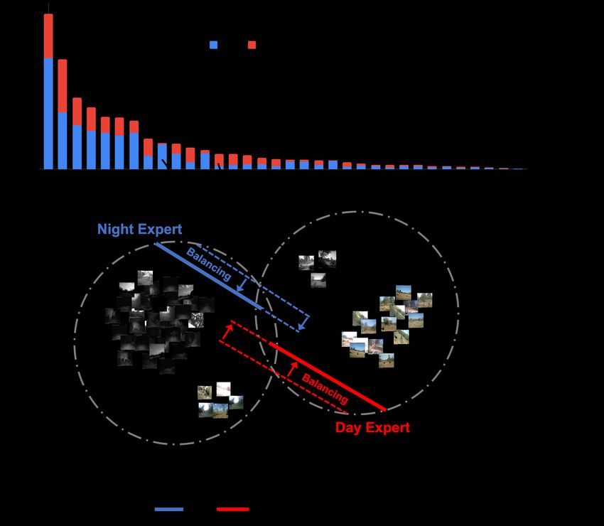
Fig. 2. Network architecture for training and inference. In the training scheme, batches are processed to estimate the past flow
f2→1 and the future flow f2→3 , and also processed to feature extractor Wθ . The output feature is then processed into each
expert EXPi (i.e., ψi ) and generate class activation map Myi . The classification loss Licls is applied for each expert, and the flow
consistency loss Lif c is applied on each expert with f2→1 and f2→3 . In the inference time, a single input image is processed
into Wθ , and the full-domain expert and the corresponding expert complement each other to output the label.

     In this paper, we propose domain experts that mitigate          bone. We use three consecutive frames as an input sequence,
the bias by combining decision boundaries, where domain ex-          and details are described in Section 3. Existing classifiers tend
perts are separately learned from each domain. There are two         to perform better on the dominant domain samples than on the
types of experts, the sub-domain expert and the full-domain          recessive domain samples; however, domain experts can miti-
expert. Exclusive sub-domain experts, one is for the night           gate the bias. Therefore, we design domain experts consisting
(i.e., IR) and the other is for the day (i.e., RGB), are indi-       of the full-domain expert and the K sub-domain experts. We
vidually specialized in that domain, and the focal loss [12]         fix K = 2 to treat day and night domain in the camera-trap
is applied to balance the imperfect decision boundary caused         setup. These two types of experts are complemented each
by the data imbalance. The full-domain expert learns from            other from two aspects: (1) The full-domain expert learns
all input images since IR and RGB images are essential for           valuable information from both domains and makes robust
learning object boundaries and contextual information, re-           predictions but is biased towards dominant domain samples;
spectively. The full-domain expert and two sub-domain ex-            (2) Sub-domain experts support the full-domain expert to pre-
perts complement each other to create better domain-balanced         dict without prejudices and give confidence to the prediction.
decision boundaries, and details are shown in Fig. 1.
     While previous methods treat successive images taken by         2.2. Training Scheme
the camera-trap as independent images, we further propose a
flow consistency loss for each expert to leverage the multi-         In this section, we briefly illustrate the training scheme
frame information. We regulate the class activation map of           for a input sequence S = {I1 , I2 , I3 } and experts Ψ =
multi-frames following the optical flow map estimated from           {ψf ull , ψday , ψnight }. Here, the domain set and the class set
pre-trained PWC-Net [13]. Thus, the flow consistency loss            are defined as D = {day, night} and C = {1, 2, · · · , C}, re-
enhances experts to pay more attention to moving objects.            spectively. The domain z ∈ D of S is determined by ensuring
     To validate our method, we introduce two camera-trap            that the input values of each channel are identical, as IR im-
datasets, WCS-LT and DMZ-LT, which are multi-domain and              ages are gray-scale. We denote y ∈ C as the class label of S,
multi-frame with long-tailed distributions. In addition, we          and determine whether the inputs are majority samples (MJs)
evaluate the accuracy on these datasets and show that our            or minority samples (MNs) depending on whether z is the
method outperforms the previous methods for samples from             dominant domain of y.
the recessive domain as well as the dominant domain.                     While ψf ull uses all input sequences, each sub-domain
                                                                     expert uses the sequences of the corresponding domain. With
                                                                     this data split mechanism, ψday and ψnight learn the domain-
                        2. METHOD
                                                                     specific decision boundaries without being hindered by data
2.1. Network Architecture                                            imbalances between domains. Following [11, 14], we use
                                                                     ResNet-50 [3] as a backbone and define each expert ψi ∈ Ψ
The architecture of the proposed network is shown in Fig. 2,         as a residual block followed by a global average pooling layer
and multiple experts are trained in parallel with a shared back-     and a learnable weight scaling classifier. Consequently, out-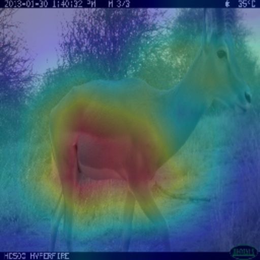
put logits before SoftMax operation of ψi are xi,1 , xi,2 , xi,3 ∈     full-domain expert ψf ull and a sub-domain expert ψz . Simi-
R1×C . To avoid interfering with each other’s learning, loss           lar to [11], the output logit xz ∈ R1×C of ψz is modified to be
functions are applied to the experts separately. First, we use         x̃z by the l2-norm of the fully-connected layer’s weights as
the focal loss [12] for ψi as the classification loss as                                     qP P
                                                                                                                z    2
                     3                                                                             k     c∈C (wk,c )
                     X                                                                 x̃z = qP P                      · xz .      (6)
         Licls = −         (1 − σ(xi,j )y )γ log(σ(xi,j )y ),    (1)                                        (w f ull 2
                                                                                                                    )
                                                                                                  k     c∈C    k,c
                     j=1
                                                                       Then, the modified output logit is averaged over two experts
where σ(xi,j )y ∈ R is the output logit of the class y after the       as
SoftMax operation for the input logit xi,j , and we fix γ = 5.                                    xf ull + x̃z
                                                                                             x=                ,                (7)
    To further increase the discriminability of each expert, a                                          2
flow consistency loss is proposed to make flow-consistent ex-          and the estimated category is defined as
perts expect to pay more attention to moving objects. We
apply the flow consistency loss for the class activation map of                           ypred = argmax (σ(x)c ).                (8)
each expert, where the class activation map of multiple frames                                      c∈C
to have a flow-consistent with the optical flow map estimated
in the pre-trained PWC-Net [13].                                                    3. CAMERA-TRAP DATASETS
    We first extract the class activation map Myij for the class
label y with the j-th frame and ψi as
                              X
                      Myij =        i
                                   wk,y Aij
                                         k,                  (2)
                                  k

         i
where wk,y   ∈ R is the fully-connected layer’s weight of ψi at
the k-th row and the y-th column, and Aij  k is the k-th chan-
nel of the feature map at the last convolution layer of ψi for                      (a)                              (b)
the j-th frame. In the context of [14], we freeze the feature
map to allow the gradient back-propagates only to the fully-
connected layer.
    With two flow maps estimated from the pre-trained PWC-
Net, a past flow map f2→1 and a future flow map f2→3 , we
generate warped maps M̂yi,1 and M̂yi,3 from Myi,1 and Myi,3 ,
respectively. Then, the flow consistency loss is applied for ψi
to match the warped maps with Myi,2 as
                                                                                                   (c)
        Lif c = Lph (Myi,2 , M̂yi,1 ) + Lph (Myi,2 , M̂yi,3 ),   (3)
                                                                       Fig. 3. iWildCAM2020 [18] statistics of (a) The number of
where Lph is a photometric consistency loss which is com-              frames per a sequence, (b) Accuracy according to the number
monly used for self-supervised optical flow and depth estima-          of frames used. (c) Long-tailed label distributions of WCS-LT
tion tasks [15, 16] as                                                 (left) and DMZ-LT (right).
                  α
   Lph (a, b) =     (1 − SSIMa,b ) + (1 − α)||a − b||1 .         (4)   We explore the relationship between the number of frames
                  2
                                                                       in a sequence and the classification accuracy since iWild-
Here, we fix α = 0.85, and SSIMa,b is the structure similar-           CAM2020 [18] provides the frame information. Given that
ity [17] between a and b. With a weight for the flow consis-           camera-traps capture images during the object moves, Fig.
tency loss β = 0.02, the overall loss function for ψi is defined       3(a) shows that most sequences consisting of up to three
as                                                                     frames capture dynamic objects, and the rest of the sequences
                     Li = Licls + βLif c .                    (5)      capture barely moving objects. Also, we observe that neu-
                                                                       ral networks overfit to these redundant frames. Figure 3(b)
2.3. Inference Scheme                                                  shows the classification performance increases as more im-
                                                                       ages are used rather than one image per sequence, and the
Different from the training phase, inferences are made on one          best performance is when the first three frames are used for
image, considering the camera-trap only captures a single im-          training while the performance deteriorates when all frames
age. Depending on the domain z of the input data, we use a             are used.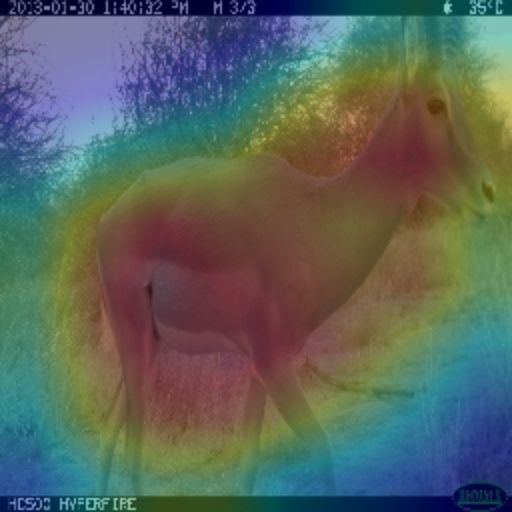
Top-1 Accuracy (%)
  Dataset            Method                                                    Major                           Minor
                                      Many    Medium      Few                                                                       All
                                                                    Balance   Imbalance Total Balance         Imbalance    Total
              baseline (ResNet-50)    88.0      60.6     36.9        79.3        66.5     77.9   81.3           59.8       78.8     78.4
                 Focal loss [12]      89.7      62.2     39.9        82.2        67.9     80.6   82.4           57.6       79.6     80.1
                   CB loss [6]        89.2      58.9     36.9        80.0        70.5     79.0   81.0           58.9       78.5     78.7
  WCS-LT
               LDAM+DRW [7]           88.9      62.1     44.4        80.1        67.9     78.7   83.1           61.2       80.7     79.7
              ACE (3 experts) [11]    80.4      59.9     62.6        74.8        69.6     74.2   77.0           52.7       74.2     74.2
                      Ours            89.8      66.6     52.0        82.2        75.5     81.4   84.6           64.7       82.4     81.9
              baseline (ResNet-50)    50.0      59.6      -          50.6        89.9     51.7   51.8           37.7       51.4     51.5
                 Focal loss [12]      48.8      59.8      -          49.4        88.4     50.4   51.1           39.1       50.7     50.6
                   CB loss [6]        51.1      45.1      -          51.0        78.3     51.7   49.7           14.5       48.8     50.2
  DMZ-LT
               LDAM+DRW [7]           52.2      65.1      -          57.1        91.3     58.0   50.6           46.4       50.5     54.2
              ACE (3 experts) [11]    64.9      42.7      -          54.9        87.0     55.7   50.5           31.9       50.0     52.9
                      Ours            56.6      62.9      -          61.4        81.2     61.9   53.0           65.2       53.3     57.6

Table 1. Comparison on long-tailed camera-trap datasets, WCS-LT and DMZ-LT. We show that our proposed method out-
performs the previous methods in most evaluation metrics. Best results in each metric are in bold. Note that we except the
accuracy for the few-shot split in the DMZ-LT dataset since there is one category that belongs to the few-shot split.

     While existing camera-trap datasets [18, 19] consider con-                             4. EXPERIMENTS
secutive frames as independent images, and also disregard
prior knowledge for each domain, we introduce two bench-               4.1. Settings
marks to cover general camera-trap settings with three char-
                                                                       Implementation Details. During training, we set the base
acteristics: (1) Training on multi-frame sequences and testing
                                                                       learning rate ηf ull of the SGD optimizer to 0.01 for WCS-LT
with a single image; (2) Multi-domain with different long-
                                                                       and 0.001 for DMZ-LT for 100 epochs, and batch size is set
tailed label distributions; (3) Domain-Balanced test dataset.
                                                                       to 48. The ψf ull uses ηf ull , while the learning rate ηi of each
WCS-LT Dataset is provided by the Wildlife Conservation                sub-domain expert ψi follows the Linear Scaling Rule [20] as
Society (WCS), and Beery et al. [18] split the data by cam-
                                                                                                                  nc
                                                                                                          P
era location, focusing on predicting unseen camera-trap im-                             ηi = ηf ull · P c∈C   P i c,                   (9)
ages. We use the annotated train split of [18], which contains                                           z∈D     c∈C nz
217,959 images from 22,111 sequences where only 8,563 se-              where ncz is the number of samples for domain z and label c.
quences include animal species. Here, we use sequences with            Input images are resized to 256 × 256, flipped horizontally
at least three frames and then select the first three frames ac-       with a probability of 12 . Moreover, Lf ull updates the back-
cording to our observation. Furthermore, we filter out dom-            bone and parameters of ψf ull , and each Li only updates ψi to
inant domain samples to fit the number of recessive domain             alleviate the learning conflict.
samples to create a domain-balanced test dataset.                      Evaluation Metrics. We first evaluate the accuracy on many-
    We use 60% of filtered sequences as the training set and           shot (more than 100 samples), medium-shot (20 ∼ 100 sam-
40% as the test set, and select only categories with at least          ples), and few-shot (less than 20 samples) splits, which are
one data in each domain and each split (i.e., train and test).         generally evaluated for long-tailed recognition tasks. To bet-
The training and test set contains 7,416 and 3,990 images,             ter understand the performance of different methods for mul-
respectively, collected from 211 locations and 34 species rep-         tiple long-tailed distributions, we calculate the accuracy for
resented in the dataset.                                               major samples (MJs) and minor samples (MNs) separately.
                                                                       We further split C into a balanced class set and an imbalanced
DMZ-LT Dataset is collected from the Korean Demilitarized              class set according to the ratio of the number of samples in the
Zone (DMZ), which is currently inaccessible due to the cease-          domain, i.e., the imbalanced class set is defined as
fire. The 4,772 sequences consisting of three consecutive
                                                                                                         maxz∈D ncz

frames contain 10 species captured in 99 locations. The two                        Cimbal = c ∈ C |                    ≥ 3   .       (10)
species (i.e., elk and wild boar) account for 70% of the en-                                             minz∈D ncz
tire dataset, resulting in the highly imbalanced label distribu-       Then, we define the remaining class set as a balanced class set
tion that makes the task challenging. We also filter out domi-         Cbal . This results in 32.3% categories of WCS-LT and 30%
nant domain samples to create a domain-balanced test dataset.          categories of DMZ-LT being in Cimbal . Taken together, we
Then, we split half of the entire sequences into the training set      evaluate the accuracy for MJs and MNs of Cbal and Cimbal .
and the other half into the test set. The training set contains        Note that the average accuracy of MJs and MNs is equal to the
7,146 images, and the test set contains 5,148 images.                  total accuracy since we use the domain-balanced test dataset.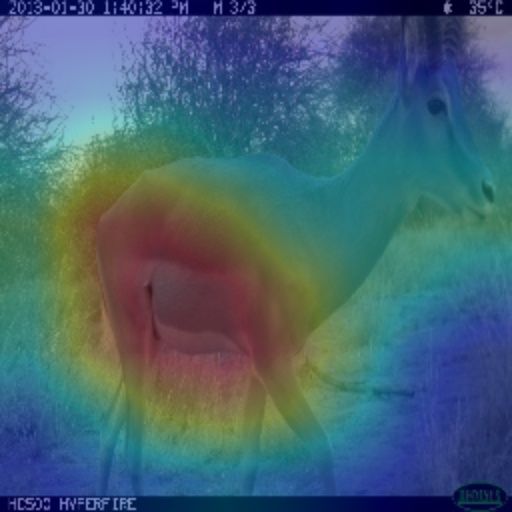
4.2. Experimental Results
In this section, we validate our proposed method with com-
parison to previous long-tailed recognition algorithms [6, 7,
11, 12], and experimental results are represented in Table 1.
For the WCS-LT dataset, our method outperforms other
methods for all evaluation metrics except for the few-shot
split. Although ACE [11] achieves the best performance on
the few-shot split, total accuracy is much lower than baseline
since the network is biased toward MJs. We achieve remark-
able improvement on MNs, exceeding the baseline by a mar-
gin of 3.3%p for Cbal and 4.9%p for Cimbal . Interestingly,
our method improves even for MJs on Cimbal by 9%p, which
means that domain experts complement each other to poten-
tiate the classification confidence for MJs.
For the DMZ-LT dataset, the difference in accuracy be-
tween MJs and MNs of Cbal is about 1%p, even MNs are
more accurate, whereas Cimbal has a difference of more than
50%p. These biases towards the dominant domain attenuate
the recessive domain prediction, leading to the shrunken deci-
sion boundary for the recessive domain. Our method exceeds
the baseline on MNs for Cimbal by a margin of 28%p, mean-
ing that the proposed framework resolves the bias even with
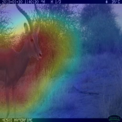
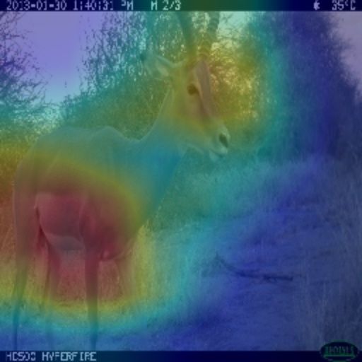
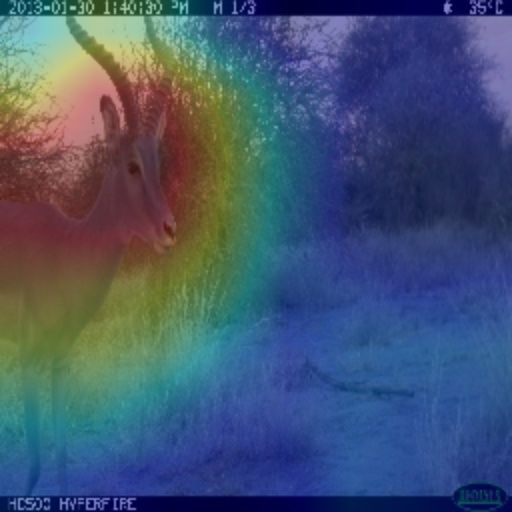
severe data imbalances. (a) Input Images (b) Focal [12] (c) Focal w/ FC (d) Ours (full) (e) Flow Maps
Fig. 4. Visualizations of class activation maps and optical
4.3. Ablation Study flow maps for ”cephalophus silvicultor”. The upper three
rows are for RGB sequences, and the lower three rows are
We also conduct an ablation study to confirm that each part
for IR sequences. Also, two consecutive flow maps for each
of our unified framework significantly improves the perfor-
domain represent f2→1 and f2→3 , respectively.
mance of camera-trap recognition.
Qualitative results in Fig. 4 indicate the flow consistency
Top-1 Accuracy (%) loss regulates the classifier to pay more attention to mov-
Baseline DE FC
Major Minor All ing objects. Specifically, our method focuses on the gen-
80.6 79.6 80.1 eral contextual information of the animal in RGB images, and
X 81.2 80.2 80.7 the class activation map of our method mainly highlights the
Focal Loss [12]
X 79.4 79.5 79.4 moving animal while the baseline focuses on the brightest ob-
X X 81.4 82.4 81.9
ject in a situation with low light conditions. In this regard,
qualitative and quantitative results strengthen the position that
Table 2. Ablation study for our proposed method on the
complementary domain experts have better discriminability
WCS-LT dataset. We use a simple long-tailed recognition
and are superior to the baseline.
method [12] as the baseline. DE means the domain-experts
and FC means the flow consistency loss. Major and Minor
metrics are the total accuracy for entire major and minor sam- 5. CONCLUSION
ples, respectively. Best results in each metric are in bold.
In this work, we have proposed a unified framework for long-
Table 2 shows the quantitative result to verify the effect tailed camera-trap recognition and introduced two bench-
of domain experts and the flow consistency loss. Domain ex- mark datasets, WCS-LT and DMZ-LT. The main contribu-
perts improve the classification performance for all evaluation tion is that domain experts are balanced through the loss re-
metrics, and further improvements are achieved when the flow weighting and complement each other to provide the domain-
consistency loss is applied to experts. Surprisingly, the flow balanced decision boundaries. We also design the flow con-
consistency loss does not address the data imbalances in base- sistency loss that experts pay more attention to moving ob-
line, but synergizes with domain experts to considerably im- jects in camera-trap images. We believe that our datasets will
prove the performance. Collectively, our unified framework contribute to camera-trap studies. In the future, we plan to
improves 1.8%p for MJs and 2.8%p for MNs compared to the extend our framework for domain generalization tasks, con-
focal loss [12]. sidering long-tailed distributions for diverse domains.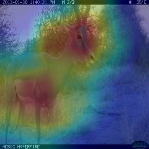
6. ACKNOWLEDGEMENT                                [10] Xudong Wang, Long Lian, Zhongqi Miao, Ziwei Liu,
                                                                     and Stella Yu, “Long-tailed recognition by routing di-
This work was supported by the National Research Founda-             verse distribution-aware experts,” in Proceedings of the
tion of Korea (NRF) grand founded by the Korea Government            International Conference on Learning Representations,
(MSIT) (NRF-2018R1A5A7025409)                                        2021.
                                                                [11] Jiarui Cai, Yizhou Wang, and Jenq-Neng Hwang,
                                                                     “Ace: Ally complementary experts for solving long-
                    7. REFERENCES                                    tailed recognition in one-shot,” in Proceedings of the
                                                                     IEEE/CVF International Conference on Computer Vi-
 [1] A Cole Burton, Eric Neilson, Dario Moreira, Andrew              sion, 2021, pp. 112–121.
     Ladle, Robin Steenweg, Jason T Fisher, Erin Bayne, and     [12] Tsung-Yi Lin, Priya Goyal, Ross Girshick, Kaiming He,
     Stan Boutin, “Wildlife camera trapping: a review and            and Piotr Dollár, “Focal loss for dense object detection,”
     recommendations for linking surveys to ecological pro-          in Proceedings of the IEEE international conference on
     cesses,” Journal of Applied Ecology, vol. 52, no. 3, pp.        computer vision, 2017, pp. 2980–2988.
     675–685, 2015.                                             [13] Deqing Sun, Xiaodong Yang, Ming-Yu Liu, and Jan
 [2] Karen Simonyan and Andrew Zisserman, “Very deep                 Kautz, “Pwc-net: Cnns for optical flow using pyramid,
     convolutional networks for large-scale image recogni-           warping, and cost volume,” in Proceedings of the IEEE
     tion,” arXiv preprint arXiv:1409.1556, 2014.                    conference on computer vision and pattern recognition,
 [3] Kaiming He, Xiangyu Zhang, Shaoqing Ren, and Jian               2018, pp. 8934–8943.
     Sun, “Deep residual learning for image recognition,” in    [14] Bingyi Kang, Saining Xie, Marcus Rohrbach, Zhicheng
     Proceedings of the IEEE conference on computer vision           Yan, Albert Gordo, Jiashi Feng, and Yannis Kalantidis,
     and pattern recognition, 2016, pp. 770–778.                     “Decoupling representation and classifier for long-tailed
 [4] Hyojun Go, Junyoung Byun, Byeongjun Park, Myung-                recognition,” in Proceedings of the Eighth International
     Ae Choi, Seunghwa Yoo, and Changick Kim, “Fine-                 Conference on Learning Representations (ICLR), 2020.
     grained multi-class object counting,” in Proceedings of    [15] Rico Jonschkowski, Austin Stone, Jonathan T Barron,
     the 2021 IEEE International Conference on Image Pro-            Ariel Gordon, Kurt Konolige, and Anelia Angelova,
     cessing (ICIP). IEEE, 2021, pp. 509–513.                        “What matters in unsupervised optical flow,” in Pro-
 [5] Mohammad Sadegh Norouzzadeh, Anh Nguyen, Mar-                   ceedings of the European Conference on Computer Vi-
     garet Kosmala, Alexandra Swanson, Meredith S Palmer,            sion. Springer, 2020, pp. 557–572.
     Craig Packer, and Jeff Clune, “Automatically identify-     [16] Clément Godard, Oisin Mac Aodha, Michael Firman,
     ing, counting, and describing wild animals in camera-           and Gabriel J Brostow, “Digging into self-supervised
     trap images with deep learning,” Proceedings of the             monocular depth estimation,” in Proceedings of the
     National Academy of Sciences, vol. 115, no. 25, pp.             IEEE/CVF International Conference on Computer Vi-
     E5716–E5725, 2018.                                              sion, 2019, pp. 3828–3838.
 [6] Yin Cui, Menglin Jia, Tsung-Yi Lin, Yang Song, and         [17] Zhou Wang, Alan C Bovik, Hamid R Sheikh, and Eero P
     Serge Belongie, “Class-balanced loss based on effective         Simoncelli, “Image quality assessment: from error vis-
     number of samples,” in Proceedings of the IEEE/CVF              ibility to structural similarity,” IEEE transactions on
     conference on computer vision and pattern recognition,          image processing, vol. 13, no. 4, pp. 600–612, 2004.
     2019, pp. 9268–9277.                                       [18] Sara Beery, Elijah Cole, and Arvi Gjoka,              “The
 [7] Kaidi Cao, Colin Wei, Adrien Gaidon, Nikos Arechiga,            iwildcam 2020 competition dataset,” arXiv preprint
     and Tengyu Ma, “Learning imbalanced datasets with               arXiv:2004.10340, 2020.
     label-distribution-aware margin loss,” in Proceedings      [19] Grant Van Horn, Oisin Mac Aodha, Yang Song, Yin Cui,
     of the Advances in Neural Information Processing Sys-           Chen Sun, Alex Shepard, Hartwig Adam, Pietro Perona,
     tems, 2019.                                                     and Serge Belongie, “The inaturalist species classifica-
 [8] Yang Zou, Zhiding Yu, BVK Kumar, and Jinsong Wang,              tion and detection dataset,” in Proceedings of the IEEE
     “Unsupervised domain adaptation for semantic segmen-            conference on computer vision and pattern recognition,
     tation via class-balanced self-training,” in Proceedings        2018, pp. 8769–8778.
     of the European conference on computer vision, 2018,       [20] Priya Goyal, Piotr Dollár, Ross Girshick, Pieter Noord-
     pp. 289–305.                                                    huis, Lukasz Wesolowski, Aapo Kyrola, Andrew Tul-
                                                                     loch, Yangqing Jia, and Kaiming He, “Accurate, large
 [9] Ziwei Liu, Zhongqi Miao, Xiaohang Zhan, Jiayun
                                                                     minibatch sgd: Training imagenet in 1 hour,” arXiv
     Wang, Boqing Gong, and Stella X Yu, “Large-scale
                                                                     preprint arXiv:1706.02677, 2017.
     long-tailed recognition in an open world,” in Proceed-
     ings of the IEEE/CVF Conference on Computer Vision
     and Pattern Recognition, 2019, pp. 2537–2546.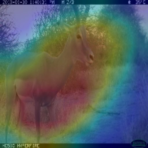
You can also read