Sensor and Sensor Fusion Technology in Autonomous Vehicles: A Review

Preprints (www.preprints.org) | NOT PEER-REVIEWED | Posted: 22 February 2021 doi:10.20944/preprints202102.0459.v1

 Review

 Sensor and Sensor Fusion Technology in
 Autonomous Vehicles: A Review
 De Jong Yeong 1,* , Gustavo Velasco-Hernandez 1 , Dr. John Barry 1 and Prof. Joseph Walsh 1
 1 IMaR Research Centre / Department of Technology, Engineering and Mathematics, Munster Technological
 University; {gustavo.velascohernandez, john.barry, joseph.walsh}@staff.ittralee.ie
 * Correspondence: de.jong.yeong@research.ittralee.ie

 Abstract: The market for autonomous vehicles (AV) is expected to experience significant growth
 over the coming decades and to revolutionize the future of transportation and mobility. The AV is
 a vehicle that is capable of perceiving its environment and perform driving tasks safely and
 efficiently with little or no human intervention and is anticipated to eventually replace conventional
 vehicles. Self-driving vehicles employ various sensors to sense and perceive their surroundings and,
 also rely on advances in 5G communication technology to achieve this objective. Sensors are
 fundamental to the perception of surroundings and the development of sensor technologies
 associated with AVs has advanced at a significant pace in recent years. Despite remarkable
 advancements, sensors can still fail to operate as required, due to for example, hardware defects,
 noise and environment conditions. Hence, it is not desirable to rely on a single sensor for any
 autonomous driving task. The practical approaches shown in recent research is to incorporate
 multiple, complementary sensors to overcome the shortcomings of individual sensors operating
 independently. This article reviews the technical performance and capabilities of sensors applicable
 to autonomous vehicles, mainly focusing on vision cameras, LiDAR and Radar sensors. The review
 also considers the compatibility of sensors with various software systems enabling the multi-sensor
 fusion approach for obstacle detection. This review article concludes by highlighting some of the
 challenges and possible future research directions.

 Keywords: autonomous vehicles; self-driving cars; perception; camera; lidar; radar; sensor fusion;
 calibration; obstacle detection;

 1. Introduction
 According to the Global Status Report published by the World Health Organization (WHO), the
 reported number of annual road traffic deaths reached 1.35 million in 2018, making it the world’s
 eighth leading cause of unnatural death among people of all ages [1]. In the context of the European
 Union (EU), while there has been a decrease in reported annual road fatalities, there is still more than
 40,000 fatalities per annum, 90% of which were caused by human error. For this reason and so as to
 improve traffic flows, global investors have invested significantly to support the development of self-
 driving vehicles. Additionally, it is expected that the autonomous vehicles (AVs) will help to reduce
 the level of carbon emissions, and hence contribute to carbon emissions reduction targets [2].
 Autonomous or driverless vehicles provide the transportation capabilities of conventional
 vehicles but are largely capable of by perceiving the environment and self-navigating with minimal
 or no human intervention. According to a report published by the Precedence Research, the global
 autonomous vehicle market size reached approximately 6,500 units in 2019 and is anticipated to
 experience a compound annual growth rate of 63.5% over the period 2020 to 2027 [3]. In 2009, Google
 secretly initiated its self-driving car project, currently known as Waymo (and presently a subsidiary
 of Google parent Alphabet). In 2014, Waymo revealed a 100% autonomous car prototype without
 pedals and steering wheel [4]. To date, Waymo has achieved a significant milestone, whereby its AVs

 © 2021 by the author(s). Distributed under a Creative Commons CC BY license.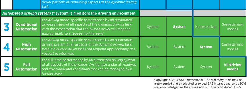

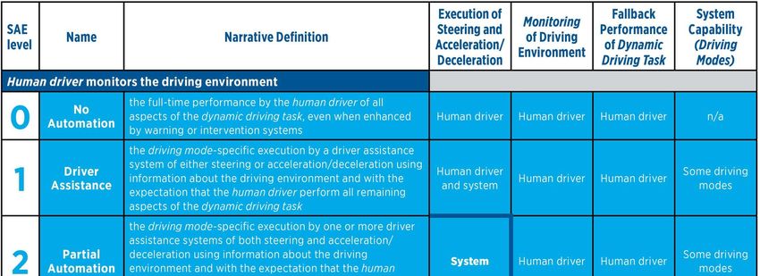
Preprints (www.preprints.org) | NOT PEER-REVIEWED | Posted: 22 February 2021 doi:10.20944/preprints202102.0459.v1

 had collectively driven over 20 million miles on public roads in 25 cities in the United States of
 America (USA) [5]. Within the Irish context, in 2020, Jaguar Land Rover (JLR) has announced its
 collaboration with autonomous car hub in Shannon, Ireland, and will use 450 km of roads to test its
 next-generation AV technology [6].
 In 2014, the SAE International, previously known as the Society of Automotive Engineers (SAE)
 introduced the J3016 “Levels of Driving Automation” standard for consumers. The J3016 standard
 defines the six distinct levels of driving automation, starting from SAE level 0 where the driver is in
 full control of the vehicle, to SAE level 5 where vehicles are capable of controlling all aspects of the
 dynamic driving tasks without human intervention. These levels are portrayed in Figure 1 and are
 often cited and referred to by industry in the safe design, development, testing, and deployment of
 highly automated vehicles (HAVs) [7]. Presently, automobile manufacturers such as Tesla and Audi
 (Volkswagen) adopted the SAE level 2 automation standards in developing its automation features,
 namely Tesla’s Autopilot [8] and Audi A8’s Traffic Jam Pilot [9,10]. Alphabet’s Waymo, on the other
 hand, has since 2016 evaluated a business model based on level 4 self-driving taxi services that could
 generate fares within a limited area in Arizona, USA [11].

 Figure 1. SAE J3016 issued in 2014 provides a common taxonomy and other definitions for automated
 driving, including full descriptions and examples for each level. Source: SAE International [7].

 While the various AV systems may vary slightly from one to the other, autonomous driving
 (AD) systems are profoundly complex systems that consists of many subcomponents. In [12], the
 architecture of an AD system is introduced from a technical perspective, which incorporates the
 hardware and software components of the AD system, and from a functional perspective, which
 describes the processing blocks required within the AV, from data collection to the control of the
 vehicle. The hardware and software are the two primary layers from the technical perspective, and
 each layer includes various subcomponents that represent different aspects of the overall system.
 Some of the subcomponents serve as a backbone within its layer for communications between the
 hardware and software layers. From the functional perspective, self-driving vehicles are composed
 of four primary functional blocks: perception, planning and decision, motion and vehicle control, and
 system supervision. These functional blocks are defined based on the processing stages and the flow

Preprints (www.preprints.org) | NOT PEER-REVIEWED | Posted: 22 February 2021 doi:10.20944/preprints202102.0459.v1

 of information from data collection to the control of the vehicle. The description of the technical and
 functional perspective of the architecture of an AV is represented in Figure 2. The detailed discussion
 of the AV architectures is beyond the scope of this paper (see [12] for a more detailed overview).

 (a) (b)
 Figure 2. Architecture of an autonomous driving (AD) system from, (a) a technical perspective that
 describes the primary hardware and software components and their implementations; (b) a functional
 perspective that describes the four main functional blocks and the flow of information based on [12].

 The sensing capabilities of an AV employing a diverse set of sensors is an essential element in
 the overall AD system; the cooperation and performance of these sensors directly determines the
 viability and safety of an AV [13]. The selection of an appropriate array of sensors and their optimal
 configurations, which will, in essence be used to imitate the human ability to perceive and formulate
 a reliable picture of the environment, is one of the primary considerations in any AD system.
 It is always essential to consider the advantages, disadvantages and limitations of the selected
 group of sensors as a whole, i.e., smart sensors and non-smart sensors. The definition of “smart sensor”
 has evolved over the past decades along with the emergence of the Internet of Things (IoT), a system
 of interrelated, internet-connected objects (devices) that can collect and transfer data over the wireless
 network without human intervention. In the IoT context, a smart sensor is a device that can condition
 the input signals, process and interpret the data, and make decisions without a separate computer
 [14]. In addition, in the AV context, range sensors for environment perception, e.g. cameras, LiDARs,
 and radars, may be considered “smart” when the sensors provide target tracking, event descriptions,
 and other information, as part of their output. In contrast, a “non-smart” sensor is a device that only
 conditions the sensor raw data or waveforms and transfers the data for remote processing. It requires
 external computing resources to process and interpret the data in order to provide additional
 information about the environment. Ultimately, a sensor is only considered “smart” when the
 computer resources is an integral part of the physical sensor design [15]. Invariably, the overall
 performance of an AV system is greatly enhanced with multiple sensors of different types
 (smart/non-smart) and modalities (visual, infrared and radio waves) operating at different range and
 bandwidth (data rate) and with the data of each being incorporated to produce a fused output
 [16,17,18]. Multi-sensor fusion is effectively now a requisite process in all AD systems, so as to
 overcome the shortcomings of individual sensor types, improving the efficiency and reliability of the
 overall AD system.
 There is currently an extensive effort invested in improving the accuracy, robustness,
 performance, and reliability of the driverless vehicle modules, not least, the operational issues related
 to cybersecurity and safety which can be crucial under real driving conditions [16]. CAVs, also known
 as Connected & Automated Vehicles, are a transformative technology that has great potential for
 reducing road accidents, improving the efficiency of transportation systems, and enhancing the
 quality of life. The connected technologies allow interactions between the automated vehicles and the
 surrounding infrastructures, for example, the on-board equipment in the CAV receives data from a
 roadside unit (RSU) and displays the appropriate alert messages to the driver. However, CAVs, along

Preprints (www.preprints.org) | NOT PEER-REVIEWED | Posted: 22 February 2021 doi:10.20944/preprints202102.0459.v1

 with other computing platforms, are susceptible to cyber-attacks and may lead to fatal crash accidents
 [19].
 This review paper will focus on the sensor modalities of an AV for environment perception, and
 an overview of the current developments and existing sensor fusion technology for object detection.
 The main purpose is to provide a comprehensive review of the technical performance and capabilities
 of sensors that are relevant to AVs and the current developments of multi-sensor fusion approaches
 for object detection in the perception subsystem. Section 2 provides an overview of the existing
 sensing modalities used in AVs, mainly focusing on vision cameras, LiDAR and radar sensors,
 including their advantages, disadvantages, and limitations in different environmental conditions.
 Section 3 discusses the necessity of sensor calibrations in AVs, an overview of an existing calibration
 package which addresses the main aspects required of any calibration system, followed by the
 current developments of sensor fusion approaches for object detection and its challenges for safe and
 reliable environment perception. Section 4 presents a summary review and outlook and
 recommendations for future research in AVs.

 2. Sensor Technology in Autonomous Vehicles
 Sensors are devices that map the detected events or changes in the surroundings to a quantitative
 measurement for further processing. In general, sensors are classified into two classes based on their
 operational principal. Proprioceptive sensors, or internal state sensors, capture the dynamical state and
 measures the internal values of a dynamic system, e.g. force, angular rate, wheel load, battery voltage,
 et cetera. Examples of the proprioceptive sensors include Inertia Measurement Units (IMU), encoders,
 inertial sensors (gyroscopes and magnetometers), and positioning sensors (Global Navigation Satellite
 System (GNSS) receivers). Conversely, the exteroceptive sensors, or external state sensors, sense and
 acquire information such as distance measurements or light intensity from the surroundings of the
 system. Cameras, Radio Detection and Ranging (Radar), Light Detection and Ranging (LiDAR), and
 ultrasonic sensors are examples of the exteroceptive sensors. Additionally, sensors can either be passive
 sensors or active sensors. Passive sensors receive energy emitting from the surroundings to produce
 outputs, e.g. vision cameras. Conversely, active sensors emit energy into the environment and measure
 the environmental ‘reaction’ to that energy to produce outputs, such as with LiDAR and radar sensors
 [20-22].
 In autonomous vehicles, sensors are critical to the perception of the surroundings and
 localization of the vehicles for path planning and decision making, essential precursors for
 controlling the motion of the vehicle. AV primarily utilizes multiple vision cameras, radar sensors,
 LiDAR sensors, and ultrasonic sensors to perceive its environment. Additionally, other sensors,
 including the Global Navigation Satellite System (GNSS), IMU, and vehicle odometry sensors are
 used to determine the relative and absolute positions of the vehicle [23]. Relative localization of an
 AV refers to the vehicles referencing of its coordinates in relation to surrounding landmarks, whereas
 absolute localization refers to the vehicle referencing its position in relation to a global reference
 frame [24]. The placement of sensors for environment perception on typical AV applications, their
 coverage, and applications are shown in Figure 3. The reader will appreciate that in a moving vehicle,
 there is a more complete coverage of the vehicles surroundings. The individual and relative
 positioning of multiple sensors are critical for precise and accurate object detection and therefore
 reliably and safely performing any subsequent actions [25]. In general, it is challenging to generate
 adequate information from a single independent source in AD. This section reviews the advantages
 and shortcomings of the three primary sensors: cameras, LiDARs and radars, for environment
 perception in AV applications.

Preprints (www.preprints.org) | NOT PEER-REVIEWED | Posted: 22 February 2021 doi:10.20944/preprints202102.0459.v1

 Figure 3. An example of the type and positioning of sensors in an automated vehicle to enable the
 vehicles perception of its surrounding. Red areas indicate the LiDAR coverage, grey areas show the
 camera coverage around the vehicle, blue areas display the coverage of short-range and medium-
 range radars, and green areas indicate the coverage of long-range radar, along with the applications
 the sensors enable; as depicted in [25] (redrawn).

 2.1. Camera
 Cameras are one of the most commonly adopted technology for perceiving the surroundings. A
 camera works on the principle of detecting lights emitted from the surroundings on a photosensitive
 surface (image plane) through a lens (mounted in front of the sensor) to produce clear images of the
 surrounding [23,26]. Cameras are relatively inexpensive and with appropriate software, are capable
 of detecting both moving and static obstacles within their field of view and provides high-resolution
 images of the surroundings. These capabilities allows the perception system of the vehicle to identify
 road signs, traffic lights, road lane markings and barriers in the case of road traffic vehicles and a host
 of other articles in the case of off-road vehicles. The camera system in an AV may employ monocular
 cameras or binocular cameras, or a combination of both. As the name implies, the monocular camera
 system utilizes a single camera to create a series of images. The conventional RGB monocular cameras
 are fundamentally more limited than binocular cameras in that they lack native depth information,
 although in some applications or more advanced monocular cameras employing the dual-pixel
 autofocus hardware, depth information may be calculated through the use of complex algorithms
 [27-29]. As a result, two cameras are often installed side-by-side to form a binocular came-ra system
 in autonomous vehicles.
 The binocular camera, also known as a stereo camera, imitates the perception of depth found in
 animals, whereby the ‘disparity’ between the slightly different images formed in each eye is (subcons-
 cisouly) employed to provide a sense of depth. Stereo cameras contain two image sensors, separated
 by a baseline. The term baseline refers to the distance between the two image sensors (and is generally
 cited in the specifications of stereo cameras), and it varies depending on the particular model of came-
 ra. For example, the Orbbec 3D cameras reviewed in [30] for Autonomous Intelligent Vehicles (AIV)
 has a baseline of 75 mm for both the Persee and Astra series cameras [31]. As in the case of animal vi-
 sion, the disparity maps calculated from stereo camera imagery permit the generation of depth maps
 using epipolar geometry and triangulation methods (detailed discussion of the disparity calculations
 algorithms is beyond the scope of this paper). Reference [32] uses the “stereo_image_proc” modules
 in Robotic Operating System (ROS), an open-source, meta-operating system for robotics [33], to perf-
 orm stereo vision processing before the implementation of SLAM (simultaneous localization and ma-
 pping) and autonomous navigation. Table 1 shows the general specifications for binocular cameras
 from different manufacturers.

Preprints (www.preprints.org) | NOT PEER-REVIEWED | Posted: 22 February 2021 doi:10.20944/preprints202102.0459.v1

 Table 1. General specifications of stereo cameras from various manufacturers that we reviewed from our initial findings. The acronyms from left to right (in second row)
 are horizontal field-of-view (HFOV); vertical field-of-view (VFOV); frames per second (FPS); image resolutions in megapixels (Img Res); depth resolutions (Res); depth
 frames per second (FPS); and reference (Ref). The ‘-‘ symbol in table below indicates that the specifications were not mentioned in product datasheet.

 Depth Information
 Baseline HFOV FPS Range Img Res Res FPS
 Model (mm) (°) VFOV (°) (Hz) (m) (MP) Range (m) (MP) (Hz) Ref
 Roboception RC Visard 160 160 61 * 48 * 25 0.5-3 1.2 0.5-3 0.03-1.2 0.8-25 [34][35]
 Carnegie
 MultiSense™ S7 1 70 80 49 / 80 30 max - 2/4 0.4 min 0.5-2 7.5-30 [34][36][37]
 Robotics®
 MultiSense™
 210 68-115 40-68 30 max - 2/4 0.4 min 0.5-2 7.5-30 [34][38]
 S21B 1
 Ensenso N35-606-16-BL 100 58 52 10 4 max 1.3 - [34][39]
 Framos D435e 55 86 57 30 0.2-10 2 0.2 min 0.9 30 [34][40]
 Nerian 0.23 / 0.45 /
 Karmin3 2 50 / 100 / 250 82 67 7 - 3 2.7 - [34][41]
 1.14 min
 Intel RealSense D455 95 86 57 30 20 max 3 0.4 min ≤1 ≤ 90
 D435 50 86 57 30 10 max 3 0.105 min ≤1 ≤ 90 [34][42]
 D415 55 65 40 30 10 max 3 0.16 min ≤1 ≤ 90
 Flir® Bumblebee2 3 120 66 - 48 / 20 - 0.3 / 0.8 [34][43]
 -
 Bumblebee XB3 3 240 66 - 16 - 1.2 [44][45]
 1HFOV, VFOV, image resolutions, image frame rates and depth information depends on the variant of focal length (optical lens geometry).
 2 Specifications stated are in full resolution and monochrome, focusing on the standard 4mm lens.

 3 Offers either 2.5mm, 3.8mm or 6mm lenses (specifications focus on 3.8mm lens) but product no longer being produced or offered (discontinued).

 * A 6mm lens has a HFOV of 43° and a VFOV of 33°.

Preprints (www.preprints.org) | NOT PEER-REVIEWED | Posted: 22 February 2021 doi:10.20944/preprints202102.0459.v1

 Other commonly employed cameras in AVs for perception of the surroundings include fisheye
 cameras [46-48]. Fisheye cameras are commonly employed in near-field sensing applications, such as
 parking and traffic jam assistance, and require only four cameras to provide a 360-degree view of the
 surroundings. Reference [46] proposed a fisheye surround-view system and the convolutional neural
 network (CNN) architecture for moving object segmentation in an autonomous driving environment,
 running at 15 frames per second at an accuracy of 40% Intersection over Union (IoU, in approximate
 terms, an evaluation metric that calculates the area of overlap between the target mask (ground truth)
 and predicted mask), and 69.5% mean IoU.
 On all practical cameras, the digital image is formed by the passage of light through the camera
 lens mounted in front of the sensor plane, which focuses and directs light rays to the sensor plane to
 form clear images of the surroundings. Deviations in lens geometry from the ideal/nominal geometry
 result in image distortion, such that in extreme cases, straight lines in the physical scene may become
 slightly curvilinear in the image. Such spatial distortion may introduce an error in the estimated
 location of detected obstacles or features in the image. Cameras are therefore usually ‘intrinsically
 calibrated’. The intrinsic calibration of all cameras is crucial so as to rectify any distortion resulting
 from the camera lens which would otherwise adversely affect the accuracy of depth perception
 measurements [49]. We present a detailed discussion of the camera intrinsic calibration and the
 commonly employed method in Section 3.1.1. Additionally, it is known that the quality (resolution)
 of images captured by the cameras may significantly affected by lighting and adverse weather
 conditions. Other disadvantages of cameras may include the requirement for large computation
 power while analyzing the image data [26].
 Given the above, cameras are a ubiquitous technology that provides high resolution videos and
 images, including color and texture information of the perceived surroundings. Common uses of the
 camera data on AVs include traffic signs recognition, traffic lights recognition, and road lane marking
 detection. As the performance of cameras and the creation of high fidelity images is highly dependent
 on the environmental conditions and illumination, image data are often fused with other sensor data
 such as radar and LiDAR data, so as to generate reliable and accurate environment perception in AD.

 2.2. LiDAR
 Light Detection and Ranging, or LiDAR, was first established in the 1960s and was widely used
 in the mapping of aeronautical and aerospace terrain. In the mid-1990s, laser scanners manufacturers
 produced and delivered the first commercial LiDARs with 2,000 to 25,000 pulses per second (PPS) for
 topographic mapping applications [50]. The development of LiDAR technologies has evolved contin-
 uously at a significant pace over the last few decades, and LiDAR is currently one of the core percepti-
 on technologies for Advanced Driver Assistance System (ADAS) and AD vehicles. LiDAR is a remote
 sensing technology that operates on principle of emitting pulses of infrared beams or laser light which
 reflect off target objects. These reflections are detected by the instrument and the interval taken betw-
 een emission and receiving of the light pulse enables the estimation of distance. As the LiDAR scans
 its surroundings, it generates a 3D representation of the scene in the form of a point cloud [26].
 The rapid growth of research and commercial enterprises relating to autonomous robots, drones,
 humanoid robots, and autonomous vehicles has created a high demand for LiDAR sensors due to its
 performance attributes such as measurement range and accuracy, robustness to surrounding changes
 and high scanning speed (or refresh rate) – for example, typical instruments in use today may register
 up to 200,000 points per second or more, covering 360° rotation and a vertical field of view of 30°. As
 a result, many LiDAR sensor companies have emerged and have been introducing new technologies
 to address these demands in recent years. Consequently, the revenue of the automotive LiDAR mark-
 et is forecasted to reach a total of 6,910 million USD by 2025 [51]. The wavelengths of the current state
 -of-the-art LiDAR sensors exploited in AVs are commonly 905nm (nanometers) – safest types of lasers
 (Class 1), which suffers lower absorption water than for example 1550nm wavelength sensors which
 were previously employed [52]. A study in reference [53] found that the 905nm systems are much ca-
 pable of providing higher resolution of point clouds in adverse weather conditions like fog and rains.
 The 905nm LiDAR systems however, are still partly sensitive to fog and precipitation: a recent study

Preprints (www.preprints.org) | NOT PEER-REVIEWED | Posted: 22 February 2021 doi:10.20944/preprints202102.0459.v1

 in [54] reported that harsh weather conditions like fogs and snows could degrade the performance of
 the sensor by 25%.
 The three primary variants of LiDAR sensors that can be applied in a wide range of applications
 include 1D, 2D and 3D LiDAR. LiDAR sensors output data as a series of points, also known as point
 cloud data (PCD) in either 1D, 2D and 3D spaces and the intensity information of the objects. For 3D
 LiDAR sensors, the PCD contains the x, y, z coordinates and the intensity information of the obstacles
 within the scene or surroundings. For AD applications, LiDAR sensors with 64- or 128- channels are
 commonly employed to generate laser images (or point cloud data) in high resolution [55,56].
  1D or one-dimensional sensors measure only the distance information (x-coordinates) of objects
 in the surroundings.
  2D or two-dimensional sensors provides additional information about the angle (y-coordinates)
 of the targeted objects.
  3D or three-dimensional sensors fire laser beams across the vertical axes to measure the elevation
 (z-coordinates) of objects around the surroundings
 LiDAR sensors can further be categorized as mechanical LiDAR or solid-State LiDAR (SSL). The
 mechanical LiDAR is the most popular long-range environment scanning solution in the field of AV
 research and development. It uses the high-grade optics and rotary lenses driven by an electric motor
 to direct the laser beams and capture the desired field of view (FoV) around the ego vehicle. The rota-
 ting lenses can achieve a 360° horizontal FoV covering the vehicle surroundings. In contrast, the SSL
 eliminate the use of rotating lenses and thereby avoid mechanical failure. SSL utilize a multiplicity of
 micro-structured waveguides to direct the laser beams to perceive the surroundings. These LiDARs
 have gained interest in recent years as an alternative to the spinning LiDARs due to their robustness,
 reliability and generally lower costs than the mechanical counterparts. However, they have a smaller
 and limited horizontal FoV, typically 120° or less, than the traditional mechanical LiDARs [23,57].
 Reference [58] compares and analyzes 12 spinning LiDAR sensors that are currently available in
 the market from various manufacturers. In [58], different models and laser configurations are evalua-
 ted in three different scenarios and environments, including dynamic traffic, adverse weather created
 in a weather simulation chamber, and static targets. The findings demonstrated that the Ouster OS1-
 16 LiDAR model had the lowest average number of points on reflective targets and the performance
 of spinning LiDARs are strong affected by intense illumination and adverse weather, notable where
 precipitation is high and there is non-uniform or heavy fog. Table 2 shows the general specifications
 of each tested LiDAR sensor in the study of [58] (comprehensive device specifications are presented
 as well in [59]). In addition, we extended the summarized general specifications in the study of [58,59]
 with other LiDARs, including Hokuyo 210° spinning LiDAR and SSLs from Cepton, SICK, and IBEO,
 and the commonly employed ROS sensor drivers for data acquisition from our initial findings.
 Laser returns are discrete observations that are recorded when a laser pulse is intercepted and
 reflected by the targets. LiDARs can collect multiple returns from the same laser pulse and modern
 sensors can record up to five returns from each laser pulse. For instance, the Velodyne VLP-32C LiDAR
 analyzes multiple returns and reports either the strongest return, the last return, or dual returns,
 depending on the laser return mode configurations. In single laser return mode (strongest return or
 last return), the sensor analyzes lights received from the laser beam in one direction to determine the
 distance and intensity information and; subsequently employs this information to determine the last
 return or strongest return. Contrarily, a sensor in dual return mode will return both the strongest and
 last return measurements. However, the second-strongest measurements will return as the strongest
 if the strongest return measurements are similar to the last return measure-ments. Not to mention
 that points with insufficient intensity will be disregarded [60].
 In general, at present, 3D spinning LiDARs are more commonly applied in self-driving vehicles
 to provide a reliable and precise perception of in day and night due to its broader field of view, farther
 detection range and depth perception. The acquired data in point cloud format provides a dense 3D
 spatial representation (or ‘laser image’) of the AVs’ surroundings. LiDAR sensors do not provide
 color information of the surroundings compared to the camera systems and this is one reason that
 the point cloud data is often fused with data from different sensors using sensor fusion algorithms.

Preprints (www.preprints.org) | NOT PEER-REVIEWED | Posted: 22 February 2021 doi:10.20944/preprints202102.0459.v1

 Table 2. General specifications of the tested LiDARs from [58,59] and other LiDARs that were reviewed in the current work. The acronyms from left to right (first row) are
 frames per second (FPS); accuracy (Acc.); detection range (RNG); vertical FoV (VFOV); horizontal FoV (HFOV); horizontal resolution (HR); vertical resolution (VR);
 wavelength (λ); diameter (Ø); sensor drivers for Robotic Operating System (ROS Drv.); and reference for further information (Ref.). The ‘-‘ symbol in table below indicates
 that the specifications were not mentioned in product datasheet.

 Channels FPS Acc. RNG VFOV HFOV HR VR λ Ø ROS
 Company Model or Layers (Hz) (m) (m) (°) (°) (°) (°) (nm) (mm) Drv. Ref.
 VLP-16 16 5-20 ±0.03 1…100 30 360 0.1-0.4 2 903 103.3
 [45]
 VLP-32C 32 5-20 ±0.03 1…200 40 360 0.1-0.4 0.33 1 903 103
 [61] [62]
 Mechanical/Spinning LiDARs

 Velodyne HDL-32E 32 5-20 ±0.02 2…100 41.33 360 0.08-0.33 1.33 903 85.3
 [63]
 HDL-64E 64 5-20 ±0.02 3…120 26.8 360 0.09 0.33 903 223.5
 [64]
 VLS-128 Alpha Prime 128 5-20 ±0.03 max 245 40 360 0.1-0.4 0.11 1 903 165.5 -
 Pandar64 64 10,20 ±0.02 0.3…200 40 360 0.2,0.4 0.167 1 905 116 [66]
 Hesai [65]
 Pandar40P 40 10,20 ±0.02 0.3…200 40 360 0.2,0.4 0.167 1 905 116 [67]
 OS1-64 Gen 1 64 10,20 ±0.03 0.8…120 33.2 360 0.7,0.35, 0.53 850 85 [69]
 Ouster [68]
 OS1-16 Gen 1 16 10,20 ±0.03 0.8…120 33.2 360 0.17 0.53 850 85 [70]
 RoboSense RS-Lidar32 32 5,10,20 ±0.03 0.4…200 40 360 0.1-0.4 0.33 1 905 114 [71] [72]
 C32-151A 32 5,10,20 ±0.02 0.5…70 32 360 0.09, 1 905 120 [73] [74]
 LeiShen
 C16-700B 16 5,10,20 ±0.02 0.5…150 30 360 0.18,0.36 2 905 102 [75] [76]
 Hokuyo YVT-35LX-F0 - 20 3 ±0.05 3 0.3…35 3 40 210 - - 905 ◊ [77] [78]
 LUX 4L Standard 4 25 0.1 50 2 3.2 110 0.25 0.8 905 ◊ [80]
 Solid State LiDARs

 IBEO LUX HD 4 25 0.1 50 2 3.2 110 0.25 0.8 905 ◊ [79] [81]
 LUX 8L 8 25 0.1 30 2 6.4 110 0.25 0.8 905 ◊ [82]
 LD-MRS400102S01 HD 4 50 - 30 2 3.2 110 0.125…0.5 - ◊ [83]
 SICK [79]
 LD-MRS800001S01 8 50 - 50 2 6.4 110 0.125…0.5 - ◊ [84]
 Vista P60 - 10 - 200 22 60 0.25 0.25 905 ◊ [86]
 Cepton Vista P90 - 10 - 200 27 90 0.25 0.25 905 ◊ [85] [87]
 Vista X90 - 40 - 200 25 90 0.13 0.13 905 ◊ [88]
 1 Stated resolutions refer to the minimum (or finest) resolutions, as these sensors have variable angle difference between central and more apical/basal beams.
 2 The documented maximum detection range is at 10% remission rate (or reflectivity rate, is a measurement of diffuse reflection on surfaces).

 3 The indicated FPS refers to the sensor’s non-interlace mode. The detection range and accuracy stated refer to white paper detections below 15m at center of vertical scan.

 ◊ Dimension/Size of the sensors are in rectangular shape: width (W) x height (H) x depth (D) - see individual references for actual dimensions.

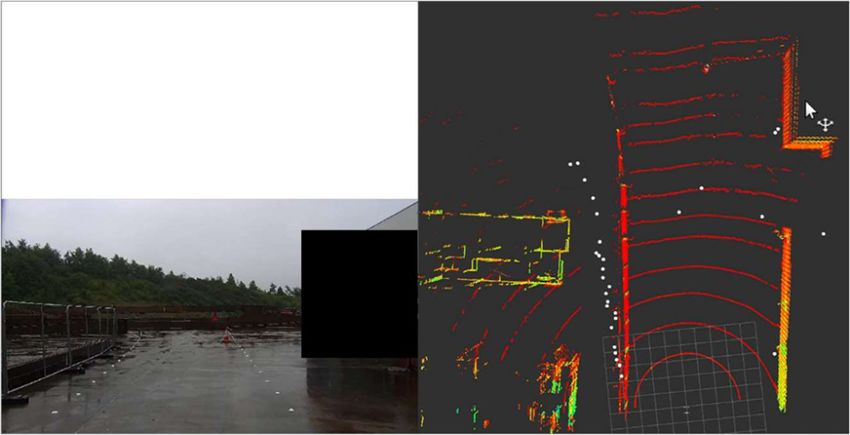
Preprints (www.preprints.org) | NOT PEER-REVIEWED | Posted: 22 February 2021 doi:10.20944/preprints202102.0459.v1

 2.3. Radar
 Radio Detection and Ranging, or Radar, was first established before World War II and operated
 on the principle of radiating electromagnetic (EM) waves within the area of interest and receiving the
 scattered waves (or reflections) of targets for further signal processing and establishing range
 information about the targets. It uses the Doppler property of EM waves to determine the relative
 speed and relative position of the detected obstacles [23], The Doppler effect, also known as Doppler
 shift, refers to the variations or shifts in wave frequency arising from relative motion between a wave
 source and its targets. For instance, the frequency of the received signal increases (shorter waves)
 when the target moves towards the direction of the radar system [89]. The general mathematical
 equation of Doppler frequency shift of a radar can be represented as [90,91]:

 2 × × 2 × 
 = = (1)
 
 where is the Doppler frequency in Hertz (Hz); is the relative speed of the target; f is the frequency
 of the transmitted signal; C is the speed of light (3 x 108 m/sec) and λ is the wavelength of the emitted
 energy. In practice, the Doppler frequency change in a radar occurs twice; firstly when the EM waves
 are emitted to the target and secondly, during the reflection of the Doppler shifted energy to the radar
 (source).
 Commercial radars available on the market currently operate at 24 GHz (Gigahertz), 60 GHz, 77
 GHz, and 79 GHz frequencies. Compared to the 79 GHz radar sensors, 24 GHz radar sensors have a
 more limited resolution of range, velocity and angle, leading to problems in identifying and reacting
 to multiple hazards and are predicted to be phased out in the future [23]. The propagation of the EM
 waves (radar) are impervious to adverse weather conditions and radar function is independent of the
 environment illumination conditions; thus, they can operate at day or night in foggy, snowy, or
 cloudy conditions. Among the drawbacks of radar sensors are the false detection of metal objects
 around the perceived surroundings like road signs or guardrails and the challenges of distinguishing
 static, stationary objects [92]. For instance, the difference between an animal carcass (static objects)
 and the road may pose a challenge for radars to resolve due to the similarity in Doppler shift [93].
 Initial findings within the present research using 79 GHz automotive radar sensor (SmartMicro [94])
 in the setup demonstrated in [94] showed a high frequency of false-positive detections in area of
 interest. Figure 4 shows an example of the false-positive detections of objects at a distance of about
 5-7 meters from the mounted sensors.

 Figure 4. Visualization (before correction for several degrees of sensor misalignment) of false-positive
 detections in current exploratory research. The colored points in the point clouds visualization repre-
 sent LiDAR point cloud data and white points represent radar point cloud data. Several false-positive
 radar detections are highlighted by the grey rectangle, located at approximately 5-7 meters from the
 radar sensor. The radar sensor in present setup is in short-range mode (maximum detection range is
 19 meters); hence, the traffic cone located at 20 meters is not detectable.

Preprints (www.preprints.org) | NOT PEER-REVIEWED | Posted: 22 February 2021 doi:10.20944/preprints202102.0459.v1

 Radar sensors in AD vehicles are commonly integrated invisibly in several locations, such as on
 the roof near the top of the windshield, behind the vehicle bumpers or brand emblems. It is essential
 to ensure the precision of mounting positions and orientations of radars in production, as any angular
 misalignment could have fatal consequences for operation of the vehicle, such errors including false
 or late detections of obstacles around the surroundings [95,96]. Medium-Range Radar (MRR), Long-
 Range Radar (LRR), and Short-Range Radar (SRR) are the three major categories of automotive radar
 systems. AV manufacturers utilize SRR for packing assistance and collision proximity warning, MRR
 for side/rear collision avoidance system and blind-spot detection and LRR for adaptive cruise control
 and early detection applications [23]. We reviewed the general specifications of several radar sensors
 from various manufacturers, such as SmartMicro, Continental, and Aptiv Delphi and an overview is
 presented in Table 3.

 Table 3. Summary of the general specifications of radar sensors from SmartMicro, Continental and
 Aptiv Delphi. The acronyms (first column from top to bottom) are frequency (Freq), horizontal FoV
 (HFOV), vertical FoV (VFOV), range accuracy (Range Acc), velocity range (Vel Range), input/output
 interfaces (IO Interfaces) and ROS (Robotic Operating System) drivers for that specific sensors. The ‘-
 ‘ symbol in table indicates that the specifications were not mentioned in product datasheet.

 Aptiv Delphi Continental SmartMicro
 ESR 2.5 SRR2 ARS 408-21 UMRR-96 T-153 1
 Freq (GHz) 76.5 76.5 76…77 79 (77…81)
 HFOV (°) ±75
 Short-Range ±9 ≥ 130
 Mid-Range ±45 ≥ 130
 Long-Range ±10 ±60 ≥ 100 (squint beam)
 VFOV (°) 4.4 10 15
 Short-Range 20
 Long-Range 14
 Range (m) 0.5-80 2
 Short-Range 0.2-70/100 0.15-19.3 3
 Mid-Range 1-60 0.4-55 3
 Long-Range 1-175 2 0.2-250 0.8-120 3
 Range Acc (m) ±0.5 noise
 Short-Range and ±0.5% < 0.15 or 1% (bigger of)
 - -
 Mid-Range bias < 0.30 or 1% (bigger of)
 Long-Range < 0.50 or 1% (bigger of)
 Vel Range (km/h) -400…+200 4
 Short-Range -400…+140 4
 - -
 Mid-Range -340…+140 4
 Long-Range -340…+140 4
 IO Interfaces CAN/Ethernet 5 PCAN CAN CAN/Automotive Ethernet
 ROS Drivers [97,98] [104] [108]
 Reference [45,99-103] [105-107] [109]
 1 It is recommended to use PCAN-USB adapter from PEAK System for connections of Controller Area
 Network (CAN) to a computer via Universal Serial Bus (USB) [110].
 2 Range indicated for ESR 2.5 (long-range mode) and SRR2 is measured at 10dB and 5dB respectively.

 3 Range may vary depending on the number of targets in the observed environment and will not achieve a

 100% true-positive detection rate.
 4 A negative velocity range indicates the object is moving away from the radar (opening range) and a positive

 value indicates the object is moving toward the radar (closing range) [111].
 5 Internet Protocol (IP) address specified on request with a sale unit and is not modifiable by user [112].

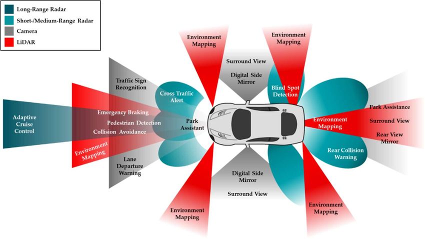
Preprints (www.preprints.org) | NOT PEER-REVIEWED | Posted: 22 February 2021 doi:10.20944/preprints202102.0459.v1

 In general, radar sensors are one of the well-known sensors in the autonomous systems, and are
 commonly employed in autonomous vehicles to provide a reliable and precise perception of obstacles
 in day and night due to its capability to function irrespective of illumination conditions and adverse
 weather conditions. It provides additional information, such as speed of the detected moving objects
 and can perform mapping in either short, medium, or long-range depending on the configuration
 mode. The radar sensor, however, is not generally suitable for object recognition applications due to
 their coarse resolutions compared to cameras. Therefore, AV researchers often fuse radar information
 with other sensory data, such as camera and LiDAR, in order to compensate for the limitations of
 radar sensors.

 3. Sensor Calibration and Sensor Fusion for Object Detection
 According to an article from Lyft Level 5, a self-driving division of Lyft in the United States [113],
 sensor calibration is one of the least discussed topics in the development of autonomous systems. It
 is the foundation block of an autonomous system and their constituent sensors, and it is a requisite
 pre-processing step before implementing sensor fusion deep learning algorithms. Sensor calibration
 informs the system about sensor position and orientation in real-world coordinates by comparing the
 relative positions of known features as detected by the radars, cameras, and LiDARs. Usually, this is
 done by adopting the intrinsic coordinate system of one of the three sensors. Precise calibrations are
 vital for further processing steps, including sensor fusion and implementation of deep learning
 algorithms for object detection, localization and mapping, and control. The term ‘object detection’
 defines the process of locating the presence of object instances (object localization) from an extensive
 number of predefined categories (image classification) in an image or a point cloud representation of
 the environment [114]. Poor calibration results may lead to the proverbial “garbage-(data)-in and
 garbage-(results)-out”; resulting in false or inaccurate estimation of the position of detected obstacles
 and may cause fatal accidents.
 Calibrations are sub-divided into intrinsic calibration, extrinsic calibration and temporal calibration.
 Intrinsic calibration addresses sensor-specific internal parameters and it is carried out first and before
 the implementation of extrinsic calibration and object detection algorithms. On the one hand, extrinsic
 calibration determines the position and orientation of sensors (rotation and translation against all the
 three orthogonal axes of 3D space) with respect to an external frame of reference. On the other hand,
 temporal calibration refers to the synchronicity of various sensor data streams with potentially different
 frequencies and latencies [115]. Section 3.1 reviews the three categories of calibrations and provides
 an overview of an existing calibration package which has been employed in the current research.
 Sensor fusion is one of the essential tasks in autonomous vehicles. Algorithms fuse information
 acquired from multiple sensors to reduce the uncertainties compared to when sensors are employed
 individually. Sensor fusion helps to build a consistent model that can perceive the surroundings
 accurately in various environment conditions [116]. The uses of sensor fusion increases the precision
 and confidence of detecting obstacles in the surroundings. In addition, it reduces the complexity and
 the overall number of components, resulting in lower overall system costs [117]. Sensor fusion
 algorithms are employed principally in the perception block of the overall architecture of an AV,
 which involves the object detections sub-processes. Reference [118] presented the Multi-Sensor Data
 Fusion (MSDF) framework for AV perceptions tasks which is depicted in Figure 5. The MSDF
 framework consists of a sensor alignment process, which involves estimating the calibration
 parameters, and several object detection processing chains (based on the number of sensors). The
 MSDF process fuses the calibration parameters and object detection information for further
 processing tasks, such as tracking, planning, and decision making. Section 3.2 reviews the three
 sensor approaches, namely high-level fusion (HLF), low-level fusion (LLF), and mid-level fusion (MLF)
 for object detection and a summary of the commonly employed algorithms, followed by the
 challenges of sensor fusion for safe and reliable environment perception.

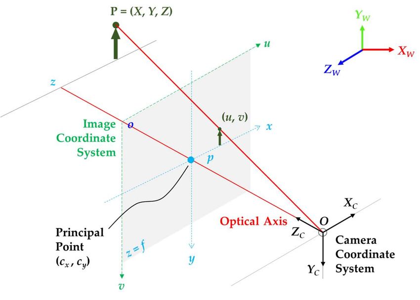
Preprints (www.preprints.org) | NOT PEER-REVIEWED | Posted: 22 February 2021 doi:10.20944/preprints202102.0459.v1

 Figure 5. The structure of Multi-Sensor Data Fusion (MSDF) framework for n given sensors. It consists
 of a sensor alignment process (estimation of calibration parameters – rotation matrix and translations
 vector) and an object detection process which contains n processing chains, each provides a list of the
 detected obstacles. Figure redrawn based on depictions in [118], but with the inclusion of an intrinsic
 calibration process.

 3.1. Sensor Calibrations

 3.1.1. Intrinsic Calibration Overview
 Intrinsic calibration is the process of determining the intrinsic parameters or internal parameters
 of a sensor which correct for systematic or deterministic aberrations or errors. These parameters are
 sensor-specific, such as focal lengths or distortion coefficients of a camera, and are expected to be con
 sistent once the intrinsic parameters are estimated. It is known through personal communication that
 Velodyne LiDARs are calibrated to 10% reflectivity (remission) of the National Institute of Standards
 and Technology (NIST) targets. Hence, the reflectance of the obstacles below the 10% reflectivity rate
 may not be detected by the LiDAR [119]. Algorithms and methods for intrinsic calibration of sensors
 have received considerable attention with significant advancement over the last number of years and
 now, are well-established in the literature. These algorithms and methodologies may vary from one
 sensor to another [120-127]. This subsection aims to provide an overview of the most commonly used
 calibration targets and the calibration methodologies for the pinhole camera model.
 The pinhole camera model is a well-known and commonly used model (inspired by the simplest
 cameras [128]) in computer vision applications, which describes the mathematical relationship of the
 projection of points in 3D space on to a 2D image plane [129]. Figure 6 visualizes the camera pinhole
 model, which consists of a closed box with a small opening (pinhole) on the front side through which
 the light rays from a target enters and produces an image on the opposing camera wall (image plane)
 [130]. From a mathematical perspective (Figure 7), the model involves a 3D camera coordinate system
 and a 2D image coordinate system to calibrate the camera using a perspective transformation method
 [132,133]. The calibration process involves utilizing the extrinsic parameters (a 3x4 matrix that consists
 of the rotation and translation [R | t] transformation) to transform the 3D points in world coordinate
 space (XW, YW, ZW) into their corresponding 3D camera coordinates (XC, YC, ZC). In addition, it involves
 employing the intrinsic parameters (also referred to as the 3x3 intrinsic matrix, K [134]), to transform
 the 3D camera coordinates into the 2D image coordinates (x, y).

Preprints (www.preprints.org) | NOT PEER-REVIEWED | Posted: 22 February 2021 doi:10.20944/preprints202102.0459.v1

 Figure 6. A graphical representation of the pinhole camera. The pinhole (aperture) restraints the light
 rays from the target from entering the pinhole; hence, affecting the brightness of the captured image
 (during image formation). A large pinhole (a wide opening) will result in a brighter image but is less
 clearer due to blurriness on both background and foreground. Figure redrawn based on depictions in
 [130,131].

 Figure 7. The pinhole camera model from a mathematical perspective. The optical axis (also referred
 to as principal axis) aligns with the Z-axis of the camera coordinate system (ZC), and the intersections
 between the image plane and the optical axis is referred to as the principal points (cx, cy). The pinhole
 opening serves as the origin (O) of the camera coordinate system (XC, YC, ZC) and the distance between
 the pinhole and the image plane is referred to as the focal length (f). Computer vision convention uses
 right-handed system with the z-axis pointing toward the target from the direction of the pinhole
 opening, while y-axis pointing downward, and x-axis rightward. Conventionally, from a viewer’s
 perspective, the origin (o) of the 2D image coordinate system (x, y) is at the top-left corner of the image
 plane with x-axis pointing rightward, and y-axis downward. The (u, v) coordinates on the image plane
 refers to the projection of points in pixels. Figure redrawn based on depictions in [123,132,133].

 The perspective transformation method outputs a 4x3 camera matrix (P), also referred to as the
 projection matrix, which comprises the intrinsic and extrinsic parameters to transform 3D world
 coordinate space into the 2D image coordinates. It should be stressed that the extrinsic calibration
 parameters in the camera calibration context differ from the extrinsic calibration process of one or
 more sensors relative to another sensor. It is known that the camera matrix does not account for any
 lens distortion – the ideal pinhole camera lacking a lens. The general mathematical equation of the
 perspective method is represented as [123,132,135,136]:

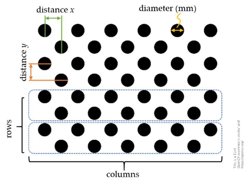
Preprints (www.preprints.org) | NOT PEER-REVIEWED | Posted: 22 February 2021 doi:10.20944/preprints202102.0459.v1

 = [R | t] or = 0 (2)
 
 0 0 1
 1

 where P is the 4x3 camera matrix; [R|t] represents the extrinsic parameters (rotation and translation)
 to transform the 3D world points (XW, YW, ZW) into camera coordinates; and K is the intrinsic matrix
 of the pinhole camera that consists of the geometry properties of a camera, such as axis skew (s),
 optical centers or principal points offset (cx, cy) and focal lengths (fx, fy). The focal length (f) of a camera
 refers to the distance between the pinhole and the image plane and it determines the projection scale
 of an image. Hence, a smaller focal length will result in a smaller image and a larger viewing angle
 [130]. A detailed discussion of the projection of 3D world points into a 2D image plane, estimation of
 camera lens distortion, and the implementations are beyond the scope of this paper (see [130,131] for
 a more comprehensive overview).
 Camera calibration (or camera re-sectioning [135]) is the process of determining the intrinsic and
 extrinsic parameters that comprise the camera matrix. Camera calibration is one of the quintessential
 issue in computer vision and photogrammetry and has received considerable attention over the last
 number of years. A variety of calibration techniques, [122-124,131,137-140] to cite a few, have been
 developed to accommodate various applications, such as AVs, Unmanned Surface Vehicle (USV) or
 underwater 3D reconstructions. Reference [139] classified these techniques into:
  Photogrammetric calibration. This approach uses the known calibration points observed from a
 calibration object (usually a planar pattern) where the geometry in the 3D world space is known
 with high precision.
  Self-calibration. This approach utilizes the correspondence between the captured images from a
 moving camera in a static scene to estimate the camera intrinsic and extrinsic parameters.
 The well-known Zhang method is one of the most used camera calibration techniques. It uses a
 combination of photogrammetric calibration and self-calibration techniques to estimate the camera
 matrix. It uses the known calibration points observed from a planar pattern (Figure 8) from multiple
 orientations (at least two) and the correspondence between the calibration points in various positions
 to estimate the camera matrix. In addition, the Zhang method for camera calibration does not require
 the motion information when either the camera or the planar pattern are moved relative to each other
 [139].

 (a) (b)
 Figure 8. The most commonly used planar patterns for camera calibration. (a) A 7 rows x 10 columns
 checkerboard pattern. The calibration uses the interior vertex points of the checkerboard pattern; thus,
 the checkerboard in (a) will utilize the 6x9 interior vertex points (some of which are circled in red)
 during calibration. (b) A 4 rows x 11 columns asymmetrical circular grid pattern. The calibration uses
 the information from circles (or “blobs” in image processing terms) detection to calibrate the camera.
 Other planar patterns include symmetrical circular grid and ChArUco patterns (a combination of
 checkerboard pattern and ArUco pattern) [126,135,139]. Figures source from OpenCV and modified.

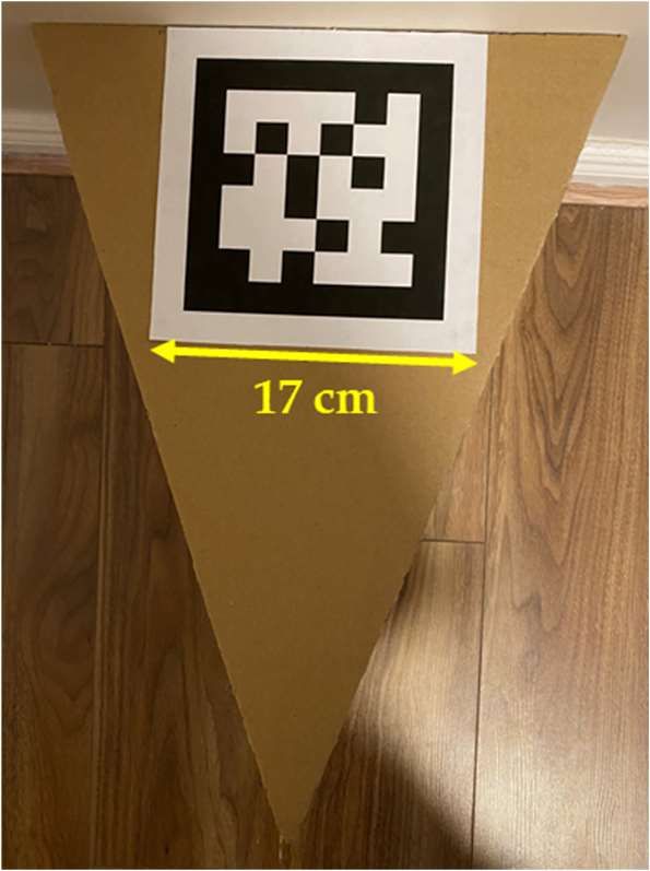
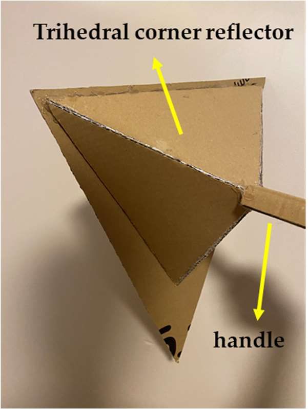
Preprints (www.preprints.org) | NOT PEER-REVIEWED | Posted: 22 February 2021 doi:10.20944/preprints202102.0459.v1

 The popular open-source “camera_calibration” package in ROS offers several pre-implemented
 scripts (executed via command line) to calibrate monocular, stereo, and fisheye cameras using the
 planar pattern as a calibration target. The calibration result includes the intrinsic matrix of a distorted
 image, distortion parameters, rectification matrix (stereo cameras only), camera matrix or projection
 matrix, and other operational parameters such as binning and region of interest (ROI). The calibration
 package was developed based on the OpenCV camera calibration and 3D reconstruction module; and
 the calibration algorithm was implemented based on the well-known Zhang method and the camera
 calibration toolbox for MATLAB by Bouguet, J.Y. [126,132].
 In general, camera calibration results are no longer applicable if the camera’s zoom (focal length)
 has changed. It should be noted that in our experience, radar and LiDAR sensors are factory intrinsic-
 calibrated.

 3.1.2. Extrinsic Calibration Overview
 Extrinsic calibration is a rigid transformation (or Euclidean transformation) that maps the points
 from one 3D coordinate system to another, for example, a rigid transformation of points from the 3D
 world or 3D LiDAR coordinate system to the 3D camera coordinate system. The extrinsic calibration
 estimates the position and orientation of the sensor relative to the orthogonal axes of 3D space (also
 known as the 6 degrees of freedoms, 6DoF) with respect to an external frame of reference [141]. The
 calibration process outputs the extrinsic parameters that consist of the rotation (R) and translation (t)
 information of the sensor and is commonly represented in a 3x4 matrix, as shown in Equation 2. This
 section aims to provide a comparative overview of the existing open-source multi-sensor extrinsic
 calibration tools and a summary of algorithms proposed in the literature for extrinsic calibration of
 camera, LiDAR, and radar sensors comprising a sensor fusion system.
 The studies of extrinsic calibration and the methodologies are well-established in the literature,
 see reference [141-149] for example. However, the extrinsic calibration of multiple sensors with
 different physical measurement principles can pose a challenge in multi-sensor systems. For instance,
 it is often challenging to match the corresponding features between camera images (dense data in
 pixels) and 3D LiDAR or radar point clouds (sparse depth data without color information) [142].
 The target-based extrinsic calibration approach employs specially designed calibration targets, such as
 marker-less planar pattern [45], checkerboard pattern [143], orthogonal and trihedral reflector
 [45,141,144-145], circular pattern to calibrate multiple sensor modalities in autonomous systems. The
 targetless extrinsic calibration approach leverages the estimated motion by individual sensors or
 utilizes the features in the perceiving environment to calibrate the sensors. However, employing the
 perceived environment features requires multimodal sensors to extract the same features within the
 environment and is sensitive to the calibration environment [142,146].
 A comparative overview of existing extrinsic calibration tools in [143] reported that the available
 tools only addressed pairwise calibrations of a maximum of two sensing modalities. For instance, the
 framework presented in [141] uses a coarse to fine extrinsic calibration approach to calibrate the RGB
 camera with a Velodyne LiDAR. The algorithm utilizes a novel 3D marker with four circular holes to
 estimate the coarse calibration parameters and further refine these parameters using the dense search
 approach to estimate a more accurate calibration in the small 6DoF calibration parameters subspace.
 Reference [147] presented an extrinsic calibration algorithm which utilizes the Planar Surface Point to
 Plane and Planar Edge to back-projected Plane geometric constraints to estimate the extrinsic parameters
 of the 3D LiDAR and a stereo camera using a marker-less planar calibration target. As highlighted in
 the previous paragraph, each sensing modality has a different physical measurement principle; thus,
 sensor setups with more modalities may duplicate the calibration efforts, especially in mobile robots
 in which sensors are frequently dismounted or repositioned. For this reason, reference [143] and [145]
 presented a novel calibration method to extrinsically calibrate all three sensing modalities, namely
 radar, LiDAR, and camera with a specially designed calibration target. Table 4 below summarizes
 the open-source extrinsic sensor calibration tools, specifically for camera, LiDAR sensor, and radar
 sensor extrinsic calibration.

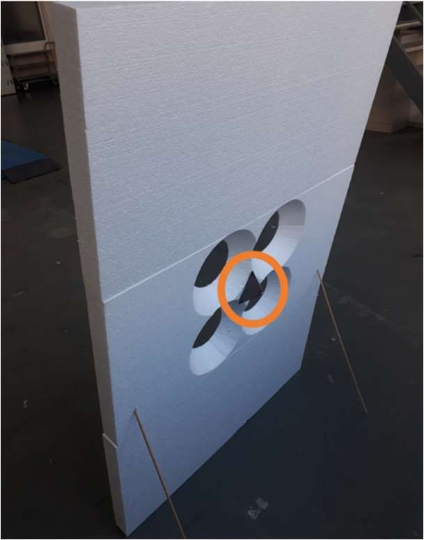
Preprints (www.preprints.org) | NOT PEER-REVIEWED | Posted: 22 February 2021 doi:10.20944/preprints202102.0459.v1

 Table 4. An overview of the available open-source extrinsic sensor calibration tools for multi-sensing
 modalities, specifically for LiDAR, radar, stereo camera and monocular camera. The acronyms of the
 columns (from left to right) are the referenced literature (Ref), stereo camera (S), monocular camera
 (M), LiDAR (L) and Radar (R). The platform and toolbox column refer to the working environment
 of the toolbox and a reference link to the open-source calibration toolbox. Further, the calibration
 target column summarizes the calibration target used for extrinsic sensor calibration. The symbols 
 and  indicate whether the proposed open-source toolbox can calibrate a particular sensor. The “*”
 symbol indicates that the proposed calibration tool claims to support monocular camera calibration.
 The “~” symbol indicates that a stereo camera could be calibrated as two separate monocular cameras,
 but in principle, it is suboptimal. The “-“ symbol indicates that the extrinsic calibration tool is not
 mentioned or openly or freely available to the research community. Based on [143] with modification.

 Ref S M L R Platform Toolbox Calibration Target
 Styrofoam planar with four circular holes and
 [143] 1  *   ROS [150]
 a copper plate trihedral corner reflector.
 Checkerboard triangular pattern with
 [145] ~    - -
 trihedral corner retroreflector.
 [149]     MATLAB [151] LiDARTag 2 and AprilTag 2.
 Planar with four circular holes and four
 [152] 3  *   ROS [153]
 ArUco markers 4 around the planar corners.
 ArUco marker on one corner of the hollow
 [155]  *   ROS [156]
 rectangular planar cardboard marker.
 [141] ~    ROS [157] 3D marker with four circular holes pattern.
 [158] ~    ROS [159] Planar checkerboard pattern.
 1 The toolbox binds with the commonly employed ROS and includes a monocular camera detector for extrinsic
 calibration, but reported results relate to stereo camera only [143].
 2 LiDARTag (point clouds) and AprilTag (images) is a visual fiducial tag (QR-code like pattern).

 3 The extrinsic calibration tool is an enhancement version of the previous work from [154].

 4 ArUco marker is a synthetic 2D square marker with a wide black border and an inner binary matrix.

 Reference [143] proposed a novel extrinsic calibration tool that utilizes a target-based calibration
 approach and a joint extrinsic calibration method to facilitate the extrinsic calibration of three sensing
 modalities. The proposed calibration target design consists of four circular, tapered holes centrally
 located within a large rectangular board and a metallic trihedral corner reflector located between the
 four circles at the rear of the board (Figure 9). The corner reflector provides a strong radar reflection
 as the Styrofoam board is largely transparent to electro-magnetic radiation. Additionally, the circular
 edges provide an accurate and robust detection for both LiDAR (especially when intersecting with
 fewer LiDAR beams) and camera. The authors of this system established three possible optimization
 configurations for joint extrinsic calibration, namely:
  Pose and Structure Estimation (PSE). It estimates the latent variables of the true board locations
 and optimizes the transformations to a precise estimate of all calibration target poses employing
 the estimated latent variables.
  Minimally Connected Pose Estimation (MCPE). It relies on a reference sensor and estimates the
 multi-sensing modalities transformations to a single reference frame.
  Fully Connected Pose Estimation (FCPE). It estimates the transformations between all sensing
 modalities “jointly” and enforces a loop closure constraint to ensure consistency.