Prequel to the Stories of Warm Conveyor Belts and Atmospheric Rivers
←
→
Page content transcription
If your browser does not render page correctly, please read the page content below
Article
Prequel to the Stories of Warm Conveyor Belts
and Atmospheric Rivers
The Moist Tongues Identified by Rossby and His Collaborators in the 1930s
Ruping Mo

                                ABSTRACT: The model of atmospheric rivers (ARs) has been around since the 1990s. A closely
                                related model is the warm conveyor belt (WCB) developed in the 1970s. Looking further back in
                                time, a phenomenon known as the “moist tongue” was intensively investigated in the late 1930s
                                and early 1940s by Rossby and his collaborators using the innovation of isentropic analysis. This
                                article aims to establish a historical perspective on the development of the moist tongue model and
                                its relevance to the current models of WCBs and ARs. As it turns out, the moist tongue was identi-
                                fied as an extension of moist air into a region of lower moisture content on the selected isentropic
                                charts. Most moist tongues are driven by large-scale cyclonic and anticyclonic eddies and are often
                                accompanied by surface cold fronts in close proximity. Ahead of the moist tongues, areas of continu-
                                ous precipitation are caused mainly by the motion of moist air up the steep isentropic slopes over
                                warm fronts or topographical features. In the warm season, the mere presence of a moist tongue
                                could be sufficient to give thunderstorms. A reanalysis dataset is used to reexamine the structures
                                and evolutions of two moist tongue events in 1936. It is shown that not all but some of the moist
                                tongues fit well with the modern conceptual models of WCB and AR. These two case studies also
                                serve to elucidate the usefulness of reanalysis data for investigating historical high-impact weather
                                events that were poorly understood due to the lack of observational data.

                                KEYWORDS: Extratropical cyclones; Atmospheric river; Jets; Synoptic-scale processes; Isotopic
                                analysis; Forecasting techniques

https://doi.org/10.1175/BAMS-D-20-0276.1
Corresponding author: Dr. R. Mo, ruping.mo@ec.gc.ca
In final form 30 December 2021
For information regarding reuse of this content and general copyright information, consult the AMS Copyright Policy.

                AMERICAN METEOROLOGICAL SOCIETY                                                                                         0 2 2 E1019
                                                                                                                           A P R I L| 2Downloaded
                                                                                                                   Unauthenticated                07/04/22 11:29 AM UTC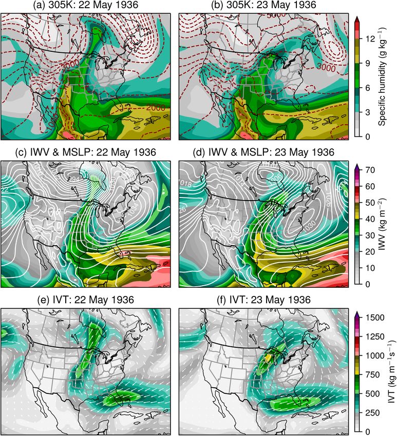
AFFILIATION: Mo—National Laboratory-West, Environment and Climate Change Canada, Vancouver,
British Columbia, Canada

T
      he atmospheric river (AR) phenomenon has been the subject of intensive research and
      applications in recent decades (Gimeno et al. 2014; Ralph et al. 2017a, 2018, 2020). This
      synoptic-scale system can be generally defined as a long (≥2,000 km), narrow (≤1,000
km), and transient corridor of strong horizontal water vapor transport concentrated in the
lower troposphere (Zhu and Newell 1998; Ralph et al. 2004). It is typically associated with
a low-level jet (LLJ) ahead of the cold front of an extratropical cyclone, and its landfall over
mountainous terrain has the potential to produce extreme precipitation and severe flooding.
The aim of this article is to build a bridge between the contemporary notion of ARs and the
concept of the moist tongue introduced by Carl-Gustaf Rossby and his colleagues in the
1930s (Rossby et al. 1937a,b). While the main motivation of Rossby’s team was to promote
isentropic analysis and show evidence of large-scale mixing in the atmosphere, their studies
also showed how isentropic charts could be used to trace the moisture from its source to the
areas of condensation and precipitation (Byers 1960).
   The terminology of AR was conceived and developed in the early 1990s. In a pilot study,
Newell et al. (1992) showed that a filamentary structure is a common feature of water vapor
transport in the troposphere. They called these filaments “tropospheric rivers” because some
may carry as much water as the Amazon. This term was soon renamed as AR by Zhu and
Newell (1994); also see Espenak and Anderson (1993, p. 12). Newell et al. (1992) noticed that
filamentary cloud bands had been documented and discussed earlier, but the associated
moisture fluxes had not been calculated (e.g., McGuirk et al. 1987; Kuhnel 1989). These cloud
bands were known as “tropical plumes” (TP) in the 1990s (McGuirk et al. 1988; McGuirk
and Ulsh 1990; Iskenderian 1995). It was also in the 1990s when “pineapple express” (PE)
emerged as a popular term in both media and academia to describe an LLJ in the northeastern
Pacific that brings warm, moist air from the area around Hawaii to the west coast of North
America (Pryne and Long 1991; Waters 1993; Davis 1995; Loukas and Quick 1996; Wood
1998; Lackmann and Gyakum 1999). The combined effect of the moist LLJ and orographic
uplift can cause some extremely heavy rainstorms in western North America (Dettinger
2004; Conrad 2009; Mo 2016). A typical example is the landfall of a PE storm during 13–15
November 2021 that triggered one of the most destructive and expensive weather disasters
in Canadian history. For just over two days, massive amounts of rain (200–300 mm in some
places with melting snow in high terrain) swamped the already soggy south coast and interior
of British Columbia, leading to widespread floods, mudslides, debris flows, and highway
washouts; this perfect storm caused the loss of at least 6 lives and close to 15,000 evacu-
ations (Environment and Climate Change Canada 2021). Note that both PE and TP storms
were referred to as “tropical moisture export” (TME) events by Knippertz and Wernli (2010).
   The first milestone for the AR theory was set by Zhu and Newell (1998), who published an
algorithm for AR identification and showed that ARs are responsible for most of the meridi-
onal moisture transport in the extratropical atmosphere. Their result indicates that ARs can
play a critical role in shaping global water and energy cycles, and their algorithm can be
used to track ARs on a daily basis in operational forecasting. Up to this time the river anal-
ogy had not been widely recognized (Davis et al. 1993; Eerme 1996; Katzfey and McInnes
1996; Iselin and Gutowski 1997; Wernli and Davies 1997), and there was concern that the

AMERICAN METEOROLOGICAL SOCIETY                                                             0 2 2 E1020
                                                                               A P R I L| 2Downloaded
                                                                       Unauthenticated                07/04/22 11:29 AM UTC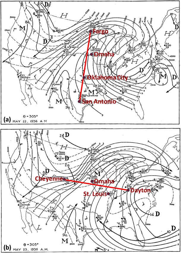
definition of “rivers” is based purely upon an Eulerian analysis, while the term implies a
Lagrangian character (Wernli 1997). It was not until the publications of Ralph et al. (2004)
that the AR notion was widely accepted and appreciated in the scientific communities (e.g.,
Smirnov and Moore 1999, 2001; Gyakum 2000; James and Houze 2005; Ralph et al. 2005,
2006; Kerr 2006; Jankov et al. 2007; Neiman et al. 2008a,b; Kaplan et al. 2009; Guan et al.
2010; Lavers et al. 2011, 2012; Sodemann and Stohl 2013; Gorodetskaya et al. 2014; Dacre
et al. 2015; Gimeno et al. 2016; Paltan et al. 2017; Zhou et al. 2018; Mo et al. 2019, 2021;
Tan et al. 2020; Ye et al. 2020; Black et al. 2021; Fu et al. 2021). The conceptual model in Ralph
et al. (2004) not only portrays the AR as a pre-cold-frontal moisture conveyor belt, but also
emphasizes its capability to produce extreme precipitation and form a critical link between
weather and climate (also see Ralph et al. 2017b).
The location of the AR along an LLJ within the warm sector of a midlatitude cyclone shares
kinematic and thermodynamic properties of a system called the warm conveyor belt (WCB),
which was recognized in the 1970s as a narrow airstream transporting large amounts of
heat, moisture, and westerly momentum (Browning 1971; Browning and Pardoe 1973;
Harrold 1973). The conceptual model of the WCB depicts a tongue of moist and warm air flow-
ing ahead of the cold front and ascending in the warm sector as it approaches the warm front
associated with a cyclone; the WCB favors heavy precipitation along the isentropes closer to
the warm front and cyclone center, where moist air rises more rapidly to achieve saturation
before joining the upper-level westerly flow (Carlson 1980; Browning 1986, 1990). The oc-
currence of heavy precipitation ahead of the cold front may also be favored when the WCB
environment provides a potential source for instability in conjunction with lift provided by the
cold front. The warm, moist air flowing along the length of the cold front is what we call the
AR today. It has been suggested that “moisture conveyor belt” could be a better term than AR
to represent strong moisture transport because it is more consistent with the well-established
WCB model (e.g., Bao et al. 2006; Knippertz and Martin 2007). To set the stage for a global
science of ARs, a workshop held in 2015 brought together experts on ARs, WCBs, and TMEs
to discuss the relationships among these interrelated concepts; the group reached consen-
sus on redefining the WCB as a zone of dynamically uplifted heat and water vapor transport
close to an extratropical cyclone, the TME as a zone of intense moisture transport out of the
tropics, and the AR as a low-level corridor of strong moisture transport that often connects a
TME to a WCB or an orographically induced rainout (Dettinger et al. 2015; Ralph et al. 2018).
Dating further back in time, we encounter the “moist tongue” (MT) and “dry tongue” (DT)
coined by Rossby et al. (1937a,b). The MT was identified as an extension of moist air into a
drier region on a selected isentropic surface. A typical example from their studies is adapted
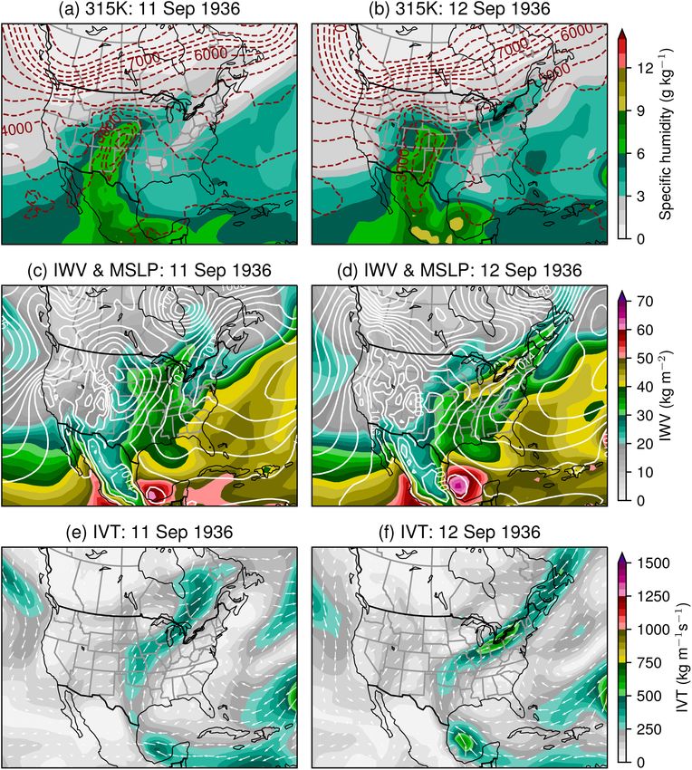
in Fig. 1, which shows an MT from the southwest intersecting a DT from the northeast on
the 315-K isentropic surface over North America in mid-September 1936. These isentropic
charts were produced by drawing on the maps the elevation contours of a selected isentropic
surface (e.g., 315 K) and the specific humidity, both interpolated from available upper-air
observations. The coherent moisture-flow pattern in Fig. 1 is often associated with cloudiness
and precipitation. Its elongated shape bears a strong resemblance to an inland-penetrating
AR across central North America (e.g., Moore et al. 2012, 2015; Mahoney et al. 2016; Mo and
Lin 2019). Note that the elevated core of a typical AR is located around 1 km above mean sea
level (MSL) (Ralph et al. 2004). Although the mean elevation of the 315-K surface in Fig. 1 is
about 3–4 km MSL, the core of the MT is below 1.5 km MSL.
Through the novel use of isentropic analysis, Rossby’s team recognized the significance
of the MTs in atmospheric dynamics and operational weather forecasting. The discovery
of this synoptic-scale feature immediately aroused extensive theoretical and practical in-
terests across the communities of meteorology, hydrology, and aviation (e.g., Osmun 1937;
Byers 1938; Wexler and Namias 1938; Namias 1938, 1939a; Denham and Knoll 1939; Rossby
AMERICAN METEOROLOGICAL SOCIETY 0 2 2 E1021
A P R I L| 2Downloaded
Unauthenticated 07/04/22 11:29 AM UTC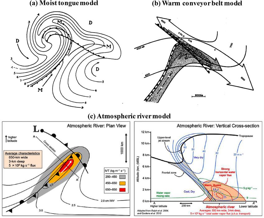
Fig. 1. The 315-K isentropic charts valid on (a) 11 and (b) 12 Sep 1936, adapted from Rossby
et al. (1937b, Figs. 4 and 5; published 1937 by the American Meteorological Society). The solid
lines are specific humidity contours (g kg−1; intervals: 2 g kg−1). The dashed lines are contours of
height (above mean sea level) of the isentropic surface in km (intervals: 0.5 km). The letters M
and D stand for moist and dry (specific humidity). The letters H (for high) and L (for low) refer to
the topography of the isentropic surface. The upper-air data used to produce these charts were
observed at the 24 aerometeorological stations indicated by dots in (b).

et al. 1939; Weightman 1939, 1940; Bernard 1940; Haynes 1940; Petterssen 1940; Swenson
1940; Knarr 1941; Mitchell and Wexler 1941; Willett et al. 1941; Starr 1942; Showalter and
Solot 1942; Means 1944; Showalter 1944). One successful application of the MT analysis was
immediately found in the forecasting of summertime precipitation. Based on a case study in
the summer of 1937, Namias (1938) pointed out that a weak MT may suffer lateral mixing
with the dry air flanking it on both sides, which could act against thunderstorm formation
and restrict the showers to its very central portion; on the other hand, strong MTs may remain
comparatively unaltered by lateral mixing, and thereby provide ideal regions for continued
thunderstorm activity (also see Rossby et al. 1938; Wexler and Namias 1938; Haynes 1940).
For winter precipitation, Namias (1939a) showed a tongue of moist and warm air flowing
northeastward over the eastern Gulf States during 6–8 December 1938; aloft, this MT was

AMERICAN METEOROLOGICAL SOCIETY                                                                0 2 2 E1022
                                                                                  A P R I L| 2Downloaded
                                                                          Unauthenticated                07/04/22 11:29 AM UTC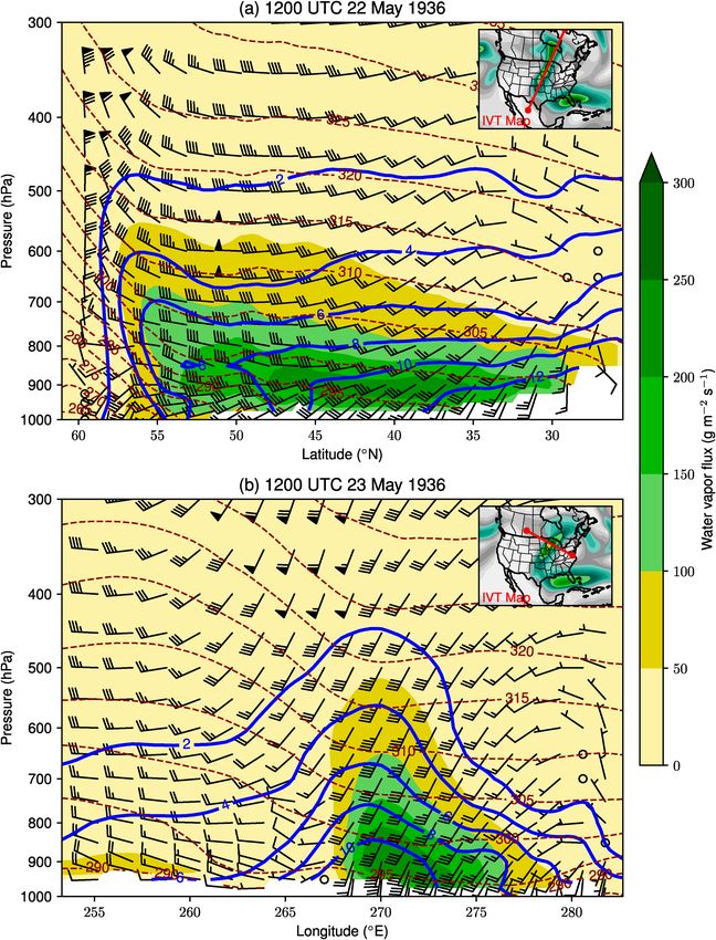
displaced by a cold DT from the west, and the established conditional instability (Rossby and
Weightman 1926) resulted in thundershowers in northern Florida.
   Unfortunately, the isentropic analysis advocated by Rossby’s team in the 1930s was sup-
planted by isobaric analysis for operational purposes after 1945, mainly because the isentropic
charts were difficult to produce in the precomputer age (for some other reasons, see Bleck 1973).
As a consequence, the enthusiasm for the isentropic MT analysis has also faded away (e.g.,
Brooks 1945; Jones and Roe 1953; Namias 1955; Semonin 1960; Fritz 1961; Leese 1962; Mills
1989; Clark et al. 2005; Cerveny et al. 2011; Jeong et al. 2014). On the other hand, MTs as a me-
teorological phenomenon have been mentioned by some researchers using the isobaric analysis
or other techniques (e.g., Takahashi et al. 1954; Saito 1966; Chang 1971; Namias and Wagner
1971; Miller 1973; Carleton 1985; Wernli 1997; Lau et al. 1998; Waugh 2005; Du et al. 2020).
   There are several important properties shared by the phenomena of MTs, WCBs, and ARs,
as conceptually illustrated in Fig. 2. They are all identified as an elongated stream of moist air.
They are often related to an extratropical cyclone and the associated fronts. Most importantly,
they all have the potential to produce heavy and sometimes prolonged precipitation. Since the
MT notion was introduced in 1937, it may be considered as a prequel to the modern theories
of WCBs (since 1971) and ARs (since 1992). It is from this historical perspective that I would
like to reexamine the classic MT model of the Rossby school and establish a connection of
this isentropic tradition with the modern theories of WCBs and ARs. There have been recent
articles that attempt to compare and distinguish among ARs, WCBs, and TMEs (e.g., Dettinger
et al. 2015; Browning 2018; Ralph et al. 2018, 2020). However, the MT model developed in
the 1930s has not received enough attention. Wernli (1997) pointed out that the analysis of
the conveyor-belt model (Browning 1971; Harrold 1973; Carlson 1980) is based on the tradi-
tional isentropic analysis developed in the 1930s (also see Wernli and Davies 1997). The term
MT was used by Browning and Hill (1985) in their isentropic analysis of the conveyor belts
associated with a polar front, and in a later study Browning (1990) recognized that the con-
veyor belt model can be related to the isentropic MT/DT model presented in Namias (1939b),
which is almost the same as Fig. 2a. This model was also cited by Ralph et al. (2004) and
Fu et al. (2021) in their AR studies. Zhu and Newell (1994) noticed the similarity between the
AR structure and a narrow tongue of moisture described by Starr (1942). Nevertheless, the
detailed features of this isentropic MT model were not sufficiently discussed in these studies.
   The first objective of this article is to present a comprehensive review of the literature related
to the identification, conceptual model, and applications of MTs in the “isentropic era.” As
expected, the isentropic MT model is indeed related to the current models of WCBs and ARs.
However, stark differences among these three phenomena do exist based in part on how they are
defined and diagnosed (e.g., isentropic, isobaric, or vertically integrated). One clear difference
is that an MT can be quite elevated and contribute to more synoptic-scale precipitation along
the WCB, whereas ARs are almost always lower tropospheric phenomena with water vapor
transport driven by the LLJ. My second objective is to demonstrate in two case studies how an
MT can be similar to an AR and how they can be quite different under certain circumstances.
Some limitations of the isentropic MT analysis will be noted and discussed in these case studies.

Isentropic charts and the moist/dry tongues
Isentropic analysis is a meteorological technique for examining air motion during an adiabatic
process above the planetary boundary layer. A common practice is to plot some variables on
a surface of constant potential temperature (isentropic surface). This approach was first sug-
gested by Sir Napier Shaw (Shaw 1929). A practical procedure for drawing isentropic weather
maps was later proposed in Shaw (1930, 259–263). The potential of this innovation was
quickly recognized by Rossby (1932), who proposed a simple graphical method for air mass
analysis by means of two conservative quantities: potential temperature and specific humidity.

AMERICAN METEOROLOGICAL SOCIETY                                                                 0 2 2 E1023
                                                                                   A P R I L| 2Downloaded
                                                                           Unauthenticated                07/04/22 11:29 AM UTC
Fig. 2. Conceptual models of the MT, WCB, and AR. (a) Schematic flow pattern around an occluded cyclone as shown by
surface fronts and moisture lines in an isentropic surface, reproduced from Namias (1940, Fig. 182, p. 364; ©McGraw Hill;
used with permission); the solid lines represent constant specific humidity (g kg−1), and the arrows indicate the instanta-
neous flow of dry (D) and moist (M) currents. (b) Conveyor belt model adapted from Browning (1971, plan view of Fig. 3,
p. 321; ©John Wiley and Sons; used with permission); stippled shading represents the warm conveyor belt and hatched
shading depicts the extent of precipitation. (c) Schematic summary of the structure and strength of an atmospheric river,
adapted from Ralph et al. (2017b, Fig. 16, p. 2594; ©American Meteorological Society; used with permission); the left panel
is a plan view, and the right panel is a vertical cross-section view.

            When the aerological network of the United States reached a state to permit a practical test
            of the value of isentropic analysis, Rossby et al. (1937a,b) took a key step by plotting specific
            humidity data on some selected isentropic surfaces. They argued that, since both potential
            temperature and specific humidity are invariant with adiabatic processes, many features of
            air motion in the free atmosphere could be visualized by plotting the specific humidity on
            isentropic surfaces. The procedure involved 1) drawing an equivalent potential temperature
            diagram for each individual airplane sounding, where the values of weather elements at a
            fixed potential temperature are determined by interpolation, and 2) plotting these values on
            a regional map for air motion analysis (Osmun 1937; Rossby et al. 1937b).
               Based on the upper-air observations from 24 aerometeorological stations across the United
            States, Rossby et al. (1937a,b) produced six isentropic charts for two synoptic situations during

            AMERICAN METEOROLOGICAL SOCIETY                                                                0 2 2 E1024
                                                                                              A P R I L| 2Downloaded
                                                                                      Unauthenticated                07/04/22 11:29 AM UTC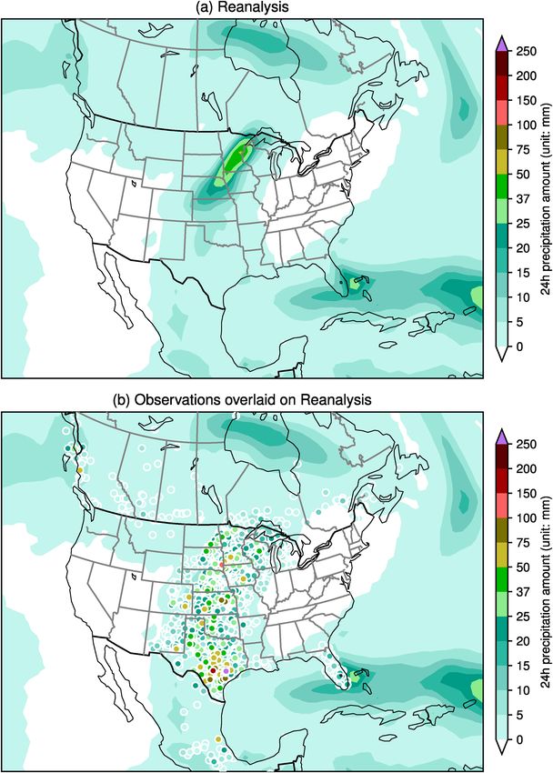
11–15 September 1936. Their first two charts are shown in Fig. 1. Note that the exact valid hour
for each map was not mentioned, because the data used to produce the map were observed
over a period of several hours. Detailed analysis of these isentropic charts led to the following
conclusions: 1) isentropic flow patterns are simpler than corresponding frontal systems on
surface maps, and they change only slowly from day to day thanks to their material nature;
2) isentropic surfaces act like material sheets over a period of a few days, except for some
small areas along active fronts or convection centers where the release of latent heat due to
condensation cannot be ignored; 3) both MTs and DTs are evident on the isentropic surfaces;
and 4) MTs or DTs advance less rapidly than expected from the observed wind distribution,
indicating intense lateral mixing in the atmosphere (the assumption of adiabatic motion
implies that each element of air remains in its proper isentropic layer).
   In particular, these two studies directed the attention of meteorologists to the large-scale MTs
and their application potential in short- and long-range weather prediction. As shown in Fig. 1a,
the situation on 11 September 1936 is characterized by the northeastward advance of an MT from
the southwestern United States on the 315-K isentropic surface. This tongue reaches the Atlantic
Coast on the next day (Fig. 1b) after having intersected a DT from the north. It was noticed that the
lines of constant specific humidity and height contour lines are nearly parallel in most areas, and
regions of vertical motion and significant precipitation may be determined from the intersection
of these two sets of lines on the isentropic charts (Rossby et al. 1937b). This statement only makes
sense for the large-scale geostrophically balanced flow. The diabatic processes associated with
strong convection and precipitation in the vicinity of a cold front may disturb the conservative
nature of the isentropic charts, because the addition of moisture through convection or loss by
precipitation cannot be avoided in some areas. As pointed out in Rossby et al. (1937a), a significant
portion of the high moisture content with the MT in Fig. 1 is likely caused by the intense vertical
mixing attending the passage of tropical air across the Mexican mountains.

Isentropic cross sections for MT analysis
Rossby et al. (1938) pointed out that the term “isentropic analysis” should apply not only to
the study of upper-air charts for prescribed isentropic surfaces, but also to the interpretation
of atmospheric cross sections, without which the analysis would be incomplete. They further
argued that, in order to take full advantage of the cross sections, it is necessary to make use
of the two most conservative properties, potential temperature (θ) and specific humidity
(q). A schematic picture of such a θ–q cross section from their study is reproduced in Fig. 3.
In these diagrams, the solid and dashed lines represent specific humidity and potential
temperature, respectively. Their usefulness for convection diagnosis was assessed by Jerome
Namias (Rossby et al. 1938, 35–36):

  The fact that convection due to heating from below lowers the isentropic surfaces but
  raises the specific humidity at any fixed level makes the isentropic cross sections espe-
  cially helpful in locating regions of significant convective activity. In these regions the
  moisture lines of the cross section bulge upward while the lines of constant potential
  temperature dip downward…

Figures 4 and 5 provide a real example adapted from Rossby et al. (1938). They were produced
from the upper-air data collected from pilot balloon ascensions for about 110 stations in North
America and some daily airplane meteorograph flights between Canada and the United States
during 22–23 May 1936. These observations were not synchronous but most of them were
taken in the morning hours between 0400 and 0800 EST (0800 and 1200 UTC). The two is-
entropic charts show an impressive MT (No. 9) extending northward from the Gulf of Mexico
to the Great Lakes region. Its shape and scale are suggestive of an inland-penetrating AR (e.g.,

AMERICAN METEOROLOGICAL SOCIETY                                                                 0 2 2 E1025
                                                                                   A P R I L| 2Downloaded
                                                                           Unauthenticated                07/04/22 11:29 AM UTC
Fig. 3. Schematic cross section through a convective area, reproduced from Rossby et al. (1938,
Fig. 4 in section B, p. 27; used with the permission of Woods Hole Oceanographic Institution). The
solid lines are specific humidity contours (g kg−1; intervals: 2 g kg−1). The dashed lines are potential
temperature contours (K; intervals: 5 K). The letters M and D stand for moist and dry. Wind speed
and direction are indicated by the conventional wind barbs.
Mo and Lin 2019). Widespread thunderstorms were reported along this moist flow. The two
isentropic cross sections show that the core of this MT was located near Earth’s surface. In
Fig. 5a, the two elevated maximum centers of specific humidity between 310 and 315 K (over
Omaha and San Antonio, respectively) were likely caused by strong convection along the MT.
Rossby et al. (1938) noticed that precipitation is often caused by the MT running up the
steep isentropic slope. Most of continuous (stratiform) precipitation occurs on the northern
side of the MTs. This is usually due to the motion of moist air up the slope of a warm front.
The distribution of thunderstorms, however, may follow the flow patterns much more closely.
Especially in the warm season, the mere presence of an MT, irrespective of whether or not it
is flowing upslope, is often sufficient to give thunderstorms.
Diabatic effects
The isentropic analysis of the Rossby school is built on the basic assumption of adiabatic mo-
tion, which implies that each element of air remains in its proper isentropic layer in the free
atmosphere. However, diabatic influences cannot always be neglected. Rossby et al. (1938)
recognized three fundamental diabatic processes that may need to be addressed carefully in
isentropic analysis: 1) radiation, 2) convection, and 3) condensation and evaporation. Their
discussions related to radiation and the diabatic effects of precipitation processes are omitted
here for clarity. Convection needs more attention; it is an important diabatic process involving
strong vertical (cross-isentrope) mass transport.
The role of convection is to transfer heat and moisture upward through the atmosphere.
The moisture pumped aloft by convection may be carried far from its source by currents in
AMERICAN METEOROLOGICAL SOCIETY 0 2 2 E1026
A P R I L| 2Downloaded
Unauthenticated 07/04/22 11:29 AM UTCFig. 4. The 305-K isentropic charts valid the mornings of 22 and 23 May 1936, adapted from Rossby
et al. (1938, Plates XIV and XV of section C; used with the permission of Woods Hole Oceanographic
Institution). The solid lines are specific humidity contours with intervals of 1 g kg−1. The dashed lines
are height contours with intervals of 500 m. The moist (M) and dry (D) tongues are numbered and
indicated by line arrows. The two red lines and eight reference stations are added to indicate the
cross-section lines in Fig. 5.
the free atmosphere, so that the moisture lines of the cross sections in the region of violent
convection frequently display a pattern similar to the anvil structure of the thunderstorm
clouds (Rossby et al. 1938). The importance of convection in maintaining the MTs was further
emphasized by Rossby et al. (1938, 36–37):
If it were not for the replenishment of moisture by convective transport upward, the moist
tongues of the isentropic charts would soon be robbed of their vapor through lateral
mixing with the dry air flanking them on both sides. In summer time thunderstorms
may truly be considered as the life blood of the moist currents.
AMERICAN METEOROLOGICAL SOCIETY 0 2 2 E1027
A P R I L| 2Downloaded
Unauthenticated 07/04/22 11:29 AM UTCFig. 5. (a) A north–south vertical cross section (from Fargo, North Dakota, to San Antonio, Texas)
valid on 22 May 1936, adapted from Rossby et al. (1938, Plate V of section C). (b) A west–east
vertical cross section (from Cheyenne, Wyoming, to Dayton, Ohio) valid on 23 May 1936, adapted
from Rossby et al. (1938, Plate VI of section C). The solid lines are specific humidity contours (inter-
vals: 1 g kg−1). The dashed lines are potential temperature contours (intervals: 5 K). The letters M
and D stand for moist and dry. Winds are indicated by the conventional wind barbs. These figures
are used with the permission of Woods Hole Oceanographic Institution.
The interactions of MTs with anticyclonic and cyclonic eddies
The interactions among MTs, DTs, cyclones, and anticyclones formed an important part of
the isentropic analysis in the 1930s. It was suggested in Rossby et al. (1938, p. 29) that the
AMERICAN METEOROLOGICAL SOCIETY 0 2 2 E1028
A P R I L| 2Downloaded
Unauthenticated 07/04/22 11:29 AM UTCformation of large-scale anticyclones and cyclones could be explained based on the principle
of conservation of absolute circulation:
Thus the total absolute circulation of any isentropic fluid chain consists of a circulation
relative to the earth plus the circulation of the earth itself about this chain. If there are
no frictional forces and if the motion is strictly adiabatic this sum must remain constant.
Thus, if an originally stationary isentropic fluid chain is displaced from equatorial to
polar regions it must develop an anticyclonic sense of circulation relative to an observer
on the earth in order to counterbalance the increased circulation of the earth itself
around the chain as it moves northward. Similarly, a southward moving system tends
to develop a cyclonic circulation.
The above statement is just the Bjerknes circulation theorem (Bjerknes 1898, 1902) applied
on an isentropic surface. It was the basis for the Rossby wave theory to be developed in
the years to come (Rossby 1939, 1940, 1941; Hoskins et al. 1985). For its application to
the MT/DT analysis, Namias (1940, p. 147) used a schematic flow pattern (see Fig. 2a) to
summarize the main features of a typical MT and its interactions with other components
surrounding an occluded cyclone:
The moist current, having come up from the south, tends to acquire anticyclonic cur-
vature indicated by the directional flow arrow to the upper right… Where the polar air
intrudes into the system from the north it develops cyclonic vorticity… Thus a branch of
the moist flow is diverted from the mother current into the cyclonic flow…
This description bears a close resemblance to the intersection of the warm and cold flows
in the conveyor belt model developed a few decades later (e.g., Browning 1971, 1986; Carlson
1980; Stewart and Macpherson 1989). Martínez-Alvarado et al. (2014) found that the WCB of
an extratropical cyclone generally splits into two branches; whether it turns cyclonically or
anticyclonically depends on the altitude at which air exits the WCB. In Fig. 2a, the MT ahead
of the cold front is what we call an AR today.
Comparisons of MTs with ARs: Two case studies
Despite the apparent similarity between the MT model and the AR (or WCB) model (Fig. 2), there
are important differences in pattern recognition, classification, and practical applications. MTs
can be visually recognized as some elongated areas of maximum specific humidity on selected
isentropic charts. Their shape and intensity may vary significantly depending on the selected
isentropic surface, and it is not easy to define lateral boundaries for an MT. The ARs, on the other
hand, are often objectively identified from the distributions of vertically integrated water vapor
(IWV) or integrated vapor transport (IVT) with some specific criteria. A popular method known
as IWV20 defines an AR as an area with IWV greater than 20 kg m−2, narrower than 1,000 km,
and longer than about 2,000 km (Ralph et al. 2004). This method has since been replaced by the
IVT methods that use both restrictive thresholds (e.g., the IVT250 in Rutz et al. 2014) and flexible
thresholds [e.g., the location and season dependent 85th percentile in Guan and Waliser (2019)];
see Shields et al. (2018) for an in-depth comparison of various AR identification techniques.
In this section, two case studies are performed to show how an MT can sometimes overlap
with or distinguish from an AR. The first case is the synoptic situation during 22–23 May
1936 (Figs. 4 and 5). The second case is the situation during 11–12 September 1936 (Fig. 1).
Data description. Two datasets are used in these two case studies. The first is version 3 of
the NOAA–CIRES–DOE Twentieth Century Reanalysis (20CRv3) produced by an assimilation
AMERICAN METEOROLOGICAL SOCIETY 0 2 2 E1029
A P R I L| 2Downloaded
Unauthenticated 07/04/22 11:29 AM UTCsystem that assimilates only surface pressure reports with observed monthly sea surface tem-
perature and sea ice distributions to generate a global atmospheric dataset (Compo et al. 2011;
Slivinski et al. 2019). This reanalysis provides 8-times daily data from 1836 to 2015 on a 1° lati-
tude × 1° longitude grid. It can reliably produce atmospheric estimates on scales ranging from
weather events to long-term climatic trends (Slivinski et al. 2021). The isentropic analysis and
vertical integration scheme can be easily performed using this three-dimensional (3D) dataset.
There are some known issues with 20CRv3, including a systematic bias in tropical precipi-
tation (Slivinski et al. 2019) and substantial biases in temperature and wind above 300 hPa
(Slivinski et al. 2021). Note that the isentropic analysis in the 1930s relied on the upper-air
data from the newly established aerological network in North America. These upper-air data,
however, were not included for assimilation to produce 20CRv3. This limitation could have an
impact on the MT and AR analyses in the case studies. In addition, the coarse resolution (1° × 1°)
would render 20CRv3 inappropriate for analyzing convective precipitation.
The second dataset includes the daily precipitation amount in North America. It is extracted
from the Global Historical Climate Network-Daily (GHCN-Daily) summaries provided by the
National Centers for Environmental Information (www.ncdc.noaa.gov/cdo-web/). This quality-
controlled dataset includes daily observations around the world. It is developed to meet the
needs of climate analysis and monitoring studies at a submonthly time resolution.
Case 1: MTs and ARs during 22–23 May 1936. The 305-K isentropic charts for the mornings
of 22 and 23 May 1936 in Fig. 4 are adapted from Rossby et al. (1938). Their reanalysis coun-
terparts (20CRv3 valid at 1200 UTC) are shown in Figs. 6a and 6b. A comparison between
them indicates that the geographical positions of the MTs are consistent. However, the ones
in Fig. 4 are drier than those in Fig. 6. For instance, the maximum specific humidity across
the U.S.–Mexico border (western Texas) is higher than 11 g kg−1 in Fig. 6a, but lower than
10 g kg−1 in Fig. 4a. A possible explanation for this difference is that the upper-air data are not
assimilated into 20CRv3, leading to incorrect estimates of moisture distribution. This could
be an inherent problem associated with this reanalysis, which takes only surface pressure
observations into account (Slivinski et al. 2021).
Also shown in Fig. 6 are the distributions of mean sea level pressure (MSLP), IWV, and IVT
valid at 1200 UTC 22–23 May 1936. An inland-penetrating AR across the central United States and
eastern Canada can be identified using either the IWV20 or IVT250 rules. It was driven northeast-
ward by a weakening cyclone-anticyclone couplet. This AR is well consistent with the isentropic
MT in Figs. 6a and 6b. There was also a weak Pacific AR making landfall on the west coast of
Canada on Figs. 6d and 6f. The corresponding MT is barely noticeable, given that elevations of
the 305-K isentropic surface in that area are generally higher than 3,500 m MSL (Fig. 6b).
Figure 7 shows two vertical cross sections from 20CRv3, on which potential temperature, spe-
cific humidity, and wind are drawn in the same fashion as in Fig. 5. An extra element, the water
vapor flux, is also included to highlight the fact that AR is a corridor of strong horizontal water
vapor transport. The north–south cross section in Fig. 7a indicates that the AR core is located
in the lower atmosphere around the 900-hPa level. At the southern end, the Mexican Plateau
acts as a barrier to block moist flow from the tropical Pacific, and as a wall to guide moisture
from the Gulf of Mexico into the United States. Toward the northern end, moisture lines bulged
upward as the AR flowed onto a warm front marked by the strong horizontal gradient of potential
temperature. The west–east cross section in Fig. 7b shows that the AR was ahead of a cold front.
The prefrontal convection forced the moisture lines to bulge upward over the AR.
The corresponding 24-h precipitation amounts from the 20CRv3 and the GHCN-Daily
observations are plotted in Fig. 8. Although the reanalysis has an AR-induced maximum
center of moderate (25–50 mm) to heavy (>50 mm) precipitation in the midwestern United
States, it seriously underestimates precipitation intensity along the AR axis. In particular,
AMERICAN METEOROLOGICAL SOCIETY 0 2 2 E1030
A P R I L| 2Downloaded
Unauthenticated 07/04/22 11:29 AM UTCFig. 6. MT and AR analysis based on the 20CRv3 data valid at 1200 UTC 22 and 23 May 1936. (a),(b) The
305-K isentropic charts, where the color-filled contours (g kg−1) show the specific humidity distribution
and the red dashed lines are contours of height (above mean sea level) of the isentropic surface (m;
intervals: 500 m). (c),(d) The IWV (color filled; kg m−2) and MSLP (white solid lines; intervals: 2 hPa).
(e),(f) The vertically integrated water vapor flux (white vector) and its magnitude known as IVT (color
filled; kg m−1 s−1). The range of vertical integration for IVT is from Earth’s surface to the 100-hPa level.
much higher amounts were observed over coastal Texas, with the highest value of 273.1 mm
at Schulenburg (29.68°N, 96.86°W). Overall, there are 37 stations reporting a daily amount
greater than 50 mm, with six of them with an amount exceeding 100 mm. On the other
hand, the differences between reanalysis and observations are acceptable over Florida
and the west coast of Canada.
Case 2: MTs and ARs during 11–12 September 1936. The isentropic MT and AR analyses
from 20CRv3 for the situations on 11–12 September 1936 are shown in Figs. 9 and 10. The
reanalysis MTs in Figs. 9a and 9b are geographically consistent with, but drier than, their
counterparts in Fig. 1; the drier conditions of 20CRv3 in this case are in contrast to the moister
conditions in the previous case.
AMERICAN METEOROLOGICAL SOCIETY 0 2 2 E1031
A P R I L| 2Downloaded
Unauthenticated 07/04/22 11:29 AM UTCFig. 7. (a) A north–south vertical cross section (from Quaqtaq, Quebec, Canada, to Torreón, Mexico)
valid at 1200 UTC 22 May 1936. (b) A west–east vertical cross section (from Calgary, Alberta, Canada,
to Richmond, Virginia) valid at 1200 UTC 23 May 1936. The blue solid lines are specific humidity con-
tours (intervals: 2 g kg−1). The red dashed lines are potential temperature contours (intervals: 5 K).
The magnitude of water vapor flux is represented by color-filled contours. Winds are indicated by
the conventional wind barbs. The cross-section line is indicated by a red line in the embedded box
with IVT distribution.
The distributions of IVT in Figs. 9e and 9f (and IWV in Figs. 9c and 9d) suggest a weak to
moderate AR over eastern North America. As compared to the corresponding MTs in Figs. 9a
and 9b, the AR axis is located further to the east in the subtropical area, and the presence of
AMERICAN METEOROLOGICAL SOCIETY 0 2 2 E1032
A P R I L| 2Downloaded
Unauthenticated 07/04/22 11:29 AM UTCFig. 8. (a) Accumulated precipitation amount (mm) for a 24-h period ending at 1200 UTC 23 May
1936 based on the 20CRv3 data. (b) The color-filled value is the same as in (a), while the observed
daily precipitation amount is plotted to a colored dot; the observed amounts are plotted in as-
cending order to make sure that a heavier amount is overlaid on a lighter amount.
AR is more noticeable over eastern and Atlantic Canada, where the specific humidity values
are low on the 315-K isentropic surface with elevations higher than 5,000 m. The isentropic
analyses on the 305-K surface are shown in Figs. 10a and 10b. The MT locations on this lower
level are more consistent with the AR positions in Figs. 9e and 9f.
The reanalysis in Fig. 10c shows generally light daily precipitation (less than 25 mm)
along the MT/AR corridor, except for some moderate (25–50 mm) rains off the east coast of
Mexico where a tropical cyclone can be seen in the MSLP maps (Figs. 9c,d). There is a local
maximum of 20–25 mm in the southern Great Lake region. The observed daily precipitation
amounts are much higher (Fig. 10d). The highest amount of 135.6 mm was observed at La
Uniòn (17.98°N, 101.88°W) in southern Mexico. It is followed by an amount of 99.8 mm at
AMERICAN METEOROLOGICAL SOCIETY 0 2 2 E1033
A P R I L| 2Downloaded
Unauthenticated 07/04/22 11:29 AM UTCFig. 9. MT and AR analysis based on the 20CRv3 data valid at 1200 UTC 11 and 12 Sep 1936. (a),(b)
The 315-K isentropic charts, where the color-filled contours (g kg−1) show the specific humidity
distribution and the red dashed lines are contours of height (above mean sea level) of the isentro-
pic surface (m; intervals: 500 m). (c),(d) The IWV (color filled; kg m−2) and MSLP (white solid lines;
intervals: 2 hPa). (e),(f) The vertically integrated water vapor flux (white vector) and its magnitude
IVT (color filled; kg m−1 s−1).
Kokomo, Indiana (40.46°N, 86.18°W). The third highest amount is 93.7 mm at Council Grove,
Kansas (38.67°N, 96.50°W), and there are 31 stations with observed daily amounts greater
than 50 mm on the map.
Conclusions
Carl-Gustaf Arvid Rossby was one of the most influential atmospheric and oceanic scientists
in the twentieth century (Byers 1960). One of his scientific undertakings in the 1930s was
the investigation of large-scale lateral mixing in the atmosphere. Following an earlier sugges-
tion of Sir Napier Shaw, Rossby et al. (1937a,b) reasoned that lateral mixing would occur on
isentropic surfaces, and these isentropic charts could be taken as a working tool for synoptic
weather analysis. Using water vapor as a conservative tracer, their first application of isentropic
analysis not only provided evidence of large-scale lateral mixing in the atmosphere, but also
identified the moist tongues as an important flow pattern which can be used for tracing the
sources of atmospheric moisture. They also suggested the use of isentropic cross sections to
provide further insight into the vertical structure and dynamic stability of MTs (Rossby et al.
AMERICAN METEOROLOGICAL SOCIETY 0 2 2 E1034
A P R I L| 2Downloaded
Unauthenticated 07/04/22 11:29 AM UTCFig. 10. (a),(b) The 305-K isentropic charts valid at 1200 UTC 11 and 12 Sep 1936 (compared to the
315-K charts in Figs. 9a,b). (c) Accumulated precipitation amount (mm) for a 24-h period ending
at 1200 UTC 12 Sep 1936 based on the 20CRv3 data. (d) The color-filled value is as in (c), while the
observed daily precipitation amount is plotted to a colored dot (see Fig. 8).
1937b, 1938). The present article established a historical narrative that would acknowledge
the MT model developed in the 1930s as an antecedent to the contemporary concepts of WCB
and AR. As shown in Fig. 2, these three phenomena are interrelated with a common feature
of strong low-level moisture transport. Under certain circumstances, therefore, they are all
but different manifestations of the same thing.
Jerome Namias was one of Rossby’s most prominent collaborators in advocating for isen-
tropic analysis. He was also part of a team devoted to developing reliable methods for short-
and long-range weather forecasts (Wexler and Namias 1938; Namias 1938, 1939a,b, 1940;
Willett et al. 1941). Their studies confirmed that an MT entering the United States from the
Gulf of Mexico is an important factor to be considered in weather forecasting, and areas of
heavy precipitation are often located in the zone between MTs and DTs where the isentropic
slopes are steepest. Figure 2a is a schematic flow pattern reproduced from Namias (1940).
This model was also adopted in a textbook by Starr (1942, p. 55):
The moisture emanating from the Gulf of Mexico may flow northward and affect any
portion of the continental United States east of the Rocky Mountains… The movement of
this moist air is usually in the form of a rather narrow tongue situated above a surface
cold front so that the forward portion of the moist outbreak is found in the vicinity of a
cyclonic disturbance at the ground…
This description was quoted by Zhu and Newell (1994) to introduce the concept of AR. In fact,
this MT model (Fig. 2a) bears an even stronger resemblance to the conceptual model of WCB
proposed in Browning (1971) (Fig. 2b).
As compared to the modern AR analysis, the MT model developed in the 1930s had some
serious limitations that could have handicapped its effectiveness and chance for success.
One is that the isentropic analysis was restricted mainly over continental regions where the
AMERICAN METEOROLOGICAL SOCIETY 0 2 2 E1035
A P R I L| 2Downloaded
Unauthenticated 07/04/22 11:29 AM UTCnetwork of upper-air observations must be sufficiently dense. Therefore, offshore moisture
transport could not be accurately accommodated. Another disadvantage is that the shape and
scale of an MT could vary significantly according to the selected isentropic surfaces. These
surfaces should remain in the free atmosphere, because specific humidity may not be con-
sidered as a conservative element in the lowest layers where air motion is largely controlled
by convection and vertical mixing (Rossby et al. 1937a). It is also difficult to assign exact
boundaries to the MTs; the same applied to the WCB analysis, as noticed by Carlson (1980).
These problems were eventually addressed and reconciled over time with the development
of modern technologies. The current AR analysis has benefited from global upper-air data
collected from multiple sources, and methods to identify ARs are often based on the IWV or
IVT distributions.
The relationship between MT and AR was further investigated in two case studies using
the reanalysis data of 20CRv3. It was demonstrated that an extensive MT on an isentropic
chart is often indicative of the presence of an AR. However, some ARs may not be captured
well on certain isentropic surfaces. On the other hand, not all MTs on isentropic charts can
be identified as an AR based on the IWV or IVT criteria. It was also demonstrated that, while
caution must be used in assessing the precipitation intensity and distribution from 20CRv3,
this reanalysis dataset offers substantial potential to assess the synoptic features of historic
ARs or other high-impact weather events.
As the antecedents for the model of ARs, WCBs or MTs are concerned, I would like to end
this article with a quote from an even earlier study of Rossby and Weightman (1926):
The type discussed below, a weak depression from the Northwest slowly approaching
the lower Mississippi Valley, and there increasing in intensity under advection of warm,
moist air from the Gulf and cold air from Canada, occurs frequently…
Acknowledgments. This article originated from a presentation at the Virtual Symposium by the
International Atmospheric Rivers Conference Community, 5–9 October 2020 (https://iarc-symposium.com/).
I would like to thank Anthony Liu, Mindy Brugman, Roxanne Vingarzan, Anna Wilson, Willie Cowan,
Jorge Eiras-Barca, and Peter Black for stimulating discussions and suggestions. Dr. Shuzhan Ren
conducted an internal review of the first version. Drs. Laura Slivinski and Gilbert Compo (NOAA) are
gratefully acknowledged for their invaluable assistance related to the use and interpretation of the
20CRv3 data. ECCC librarians, Alison Dodd and Danny Chan, kindly assisted with manuscript research.
Critical and constructive comments from three anonymous reviewers are highly appreciated. Editor
Kristine Harper provided many valuable suggestions for improving the final version.
Data availability statement. The Twentieth Century Reanalysis V3 data are provided by the NOAA/
OAR/ESRL PSL, Boulder, Colorado, from their website at https://psl.noaa.gov/data/gridded/data.20thC_ReanV3.
html. Daily precipitation data across Canada, the United States, and Mexico in May and September
1936 are downloaded from Climate Data Online, www.ncdc.noaa.gov/cdo-web/, provided by the NOAA’s
National Centers for Environmental Information.
AMERICAN METEOROLOGICAL SOCIETY 0 2 2 E1036
A P R I L| 2Downloaded
Unauthenticated 07/04/22 11:29 AM UTCReferences
Bao, J.-W., S. A. Michelson, P. J. Neiman, F. M. Ralph, and J. M. Wilczak, 2006: Davis, D. D., and Coauthors, 1993: A photostationary state analysis of the NO2-
Interpretation of enhanced integrated water vapor bands associated with NO system based on airborne observations from the subtropical/tropical
extratropical cyclones: Their formation and connection to tropical moisture. North and South Atlantic. J. Geophys. Res., 98, 23 501–23 523, https://doi.
Mon. Wea. Rev., 134, 1063–1080, https://doi.org/10.1175/MWR3123.1. org/10.1029/93JD02412.
Bernard, M., 1940: The application of hydrometeorology to engineering problems. Davis, M., 1995: Los Angeles after the storm: The dialectic of ordinary disaster. An-
Proc. Hydraulics Conf., Iowa City, IA, University of Iowa, 69–80. tipode, 27, 221–241, https://doi.org/10.1111/j.1467-8330.1995.tb00276.x.
Bjerknes, V., 1898: Ueber die Bildung von Cirkulationsbewegungen und Wirbeln Denham, W. S., and D. W. Knoll, 1939: An isentropic analysis of a thunderstorm
in reibungslosen Flüssigkeiten. Vidensk.-Selsk. Skr. Mat.-Naturvidensk. Kl., situation. M.S. thesis, Massachusetts Institute of Technology, 99 pp.
No. 5, 29 pp. Dettinger, M., 2004: Fifty-two years of “pineapple-express” storms across the
——, 1902: Cirkulation relativ zu der Erde. Meteor. Z., 19, 97–108. west coast of North America. California Energy Commission Rep. CEC-500-
Black, A. S., and Coauthors, 2021: Australian northwest cloudbands and their 2005-004, 20 pp.
relationship to atmospheric rivers and precipitation. Mon. Wea. Rev., 149, ——, F. M. Ralph, and D. A. Lavers, 2015: Setting the stage for a global science
1125–1139, https://doi.org/10.1175/MWR-D-20-0308.1. of atmospheric rivers. Eos, Trans. Amer. Geophys. Union, 96, https://doi.
Bleck, R., 1973: Numerical forecasting experiments based on the conservation of org/10.1029/2015EO038675.
potential vorticity on isentropic surfaces. J. Appl. Meteor. Climatol., 12, 737– Du, Y., G. Chen, B. Han, C. Mai, L. Bai, and M. Li, 2020: Convection initiation and
752, https://doi.org/10.1175/1520-0450(1973)0122.0.CO;2. growth at the coast of South China. Part I: Effect of the marine boundary
Brooks, C. F., 1945: Report on the Kansas City meeting, Jan. 24–26, 1945. Bull. layer jet. Mon. Wea. Rev., 148, 3847–3869, https://doi.org/10.1175/MWR-
Amer. Meteor. Soc., 26, 33–47, https://doi.org/10.1175/1520-0477-26.2.33. D-20-0089.1.
Browning, K. A., 1971: Radar measurements of air motion near fronts. Part two: Eerme, K., 1996: Greenhouse gases and their impact on the radiation balance.
Some categories of frontal air motion. Weather, 26, 320–340, https://doi. Estonia in the System of Global Climate Change, Institute of Ecology, 10–16.
org/10.1002/j.1477-8696.1971.tb04211.x. Environment and Climate Change Canada, 2021: Canada’s top 10 weather sto-
——, 1986: Conceptual models of precipitation systems. Wea. Forecasting, 1, 23– ries of 2021. ECCC, www.canada.ca/en/environment-climate-change/servic-
41, https://doi.org/10.1175/1520-0434(1986)0012.0.CO;2. es/top-ten-weather-stories/2021.html.
——, 1990: Organization of clouds and precipitation in extratropical cyclones. Espenak, F., and J. Anderson, 1993: Annular solar eclipse of 10 May 1994. Na-
Extratropical Cyclones, C. W. Newton and E. O. Holopainen, Eds., Amer. Me- tional Aeronautics and Space Administration Rep. 1301, 87 pp.
teor. Soc., 129–153, https://doi.org/10.1007/978-1-944970-33-8_8. Fritz, S., 1961: Satellite cloud pictures of a cyclone over the Atlantic Ocean. Quart.
——, 2018: Atmospheric rivers in the U.K. Bull. Amer. Meteor. Soc., 99, 1108– J. Roy. Meteor. Soc., 87, 314–321, https://doi.org/10.1002/qj.49708737304.
1109, https://doi.org/10.1175/BAMS-D-17-0291.1. Fu, G., S. Liu, X. Li, P. Li, and L. Chen, 2021: Characteristics of atmospheric riv-
——, and C. W. Pardoe, 1973: Structure of low-level jet streams ahead of mid- ers over the East Asia in middle summers from 2001 to 2016. J. Ocean Univ.
latitude cold fronts. Quart. J. Roy. Meteor. Soc., 99, 619–638, https://doi. China, 20, 235–243, https://doi.org/10.1007/s11802-021-4513-x.
org/10.1002/qj.49709942204. Gimeno, L., R. Nieto, M. Vázquez, and D. A. Lavers, 2014: Atmospheric riv-
——, and F. F. Hill, 1985: Mesoscale analysis of a polar trough interacting with a ers: A mini-review. Front. Earth Sci., 2, 2, https://doi.org/10.3389/
polar front. Quart. J. Roy. Meteor. Soc., 111, 445–462, https://doi.org/10.1002/ feart.2014.00002.
qj.49711146809. ——, and Coauthors, 2016: Major mechanisms of atmospheric moisture transport
Byers, H. R., 1938: On the thermodynamic interpretation of isentropic charts. Mon. and their role in extreme precipitation events. Annu. Rev. Environ. Resour.,
Wea. Rev., 66, 63–68, https://doi.org/10.1175/1520-0493(1938)662.0.CO;2. Gorodetskaya, I. V., M. Tsukernik, K. Claes, M. F. Ralph, W. D. Neff, and N. P. M.
——, 1960: Carl-Gustaf Arvid Rossby: 1898–1957. Natl. Acad. Sci., 34, 248–270. Van Lipzig, 2014: The role of atmospheric rivers in anomalous snow accu-
Carleton, A. M., 1985: Synoptic and satellite aspects of the southwestern U.S. mulation in East Antarctica. Geophys. Res. Lett., 41, 6199–6206, https://doi.
summer ‘monsoon’. J. Climatol., 5, 389–402, https://doi.org/10.1002/ org/10.1002/2014GL060881.
joc.3370050406. Guan, B., and D. E. Waliser, 2019: Tracking atmospheric rivers globally: Spatial
Carlson, T. N., 1980: Airflow through midlatitude cyclones and the comma cloud distributions and temporal evolution of life cycle characteristics. J. Geophys.
pattern. Mon. Wea. Rev., 108, 1498–1509, https://doi.org/10.1175/1520- Res. Atmos., 124, 12523–12552, https://doi.org/10.1029/2019JD031205.
0493(1980)1082.0.CO;2. ——, N. P. Molotch, D. E. Waliser, E. J. Fetzer, and P. J. Neiman, 2010: Extreme
Cerveny, R. S., K. DeBiasse, M. B. Pace, A. W. Ellis, and R. C. Balling Jr., 2011: Re- snowfall events linked to atmospheric rivers and surface air temperature
analysis and extension of Namias’s climatological isentropic analysis: Detec- via satellite measurements. Geophys. Res. Lett., 37, L20401, https://doi.
tion and evaluation of monsoonal, severe storm, drought, and flood events. org/10.1029/2010GL044696.
Ann. Assoc. Amer. Geogr., 101, 1204–1220, https://doi.org/10.1080/000456 Gyakum, J. R., 2000: Moisture transport to Arctic drainage basins relating to sig-
08.2011.584280. nificant precipitation events and cyclogenesis. The Freshwater Budget of the
Chang, J.-H., 1971: The Chinese monsoon. Geogr. Rev., 61, 370–395, https://doi. Arctic Ocean, E. Lewis et al., Eds., Springer, 197–208.
org/10.2307/213434. Harrold, T. W., 1973: Mechanisms influencing the distribution of precipitation
Clark, P. A., K. A. Browning, and C. Wang, 2005: The sting at the end of the tail: Model within baroclinic disturbances. Quart. J. Roy. Meteor. Soc., 99, 232–251,
diagnostics of fine-scale three-dimensional structure of the cloud head. Quart. https://doi.org/10.1002/qj.49709942003.
J. Roy. Meteor. Soc., 131, 2263–2292, https://doi.org/10.1256/qj.04.36. Haynes, B. C., 1940: Meteorology for pilots. U.S. Civil Aeronautics Administration
Compo, G. P., and Coauthors, 2011: The Twentieth Century Reanalysis Project. Civil Aeronautics Bulletin 25, 150 pp.
Quart. J. Roy. Meteor. Soc., 137, 1–28, https://doi.org/10.1002/qj.776. Hoskins, B. J., M. E. McIntyre, and A. W. Robertson, 1985: On the use and signifi-
Conrad, C. T., 2009: Severe and Hazardous Weather in Canada: The Geography of cance of isentropic potential vorticity maps. Quart. J. Roy. Meteor. Soc., 111,
Extreme Events. Oxford University Press, 205 pp. 877–946, https://doi.org/10.1002/qj.49711147002.
Dacre, H. F., P. A. Clark, O. Martinez-Alvarado, M. A. Stringer, and D. A. Lavers, Iselin, J. P., and W. J. Gutowski, 1997: Water vapor layers in STORM-FEST
2015: How do atmospheric rivers form? Bull. Amer. Meteor. Soc., 96, 1243– rawinsonde observations. Mon. Wea. Rev., 125, 1954–1963, https://doi.
1255, https://doi.org/10.1175/BAMS-D-14-00031.1. org/10.1175/1520-0493(1997)1252.0.CO;2.
AMERICAN METEOROLOGICAL SOCIETY 0 2 2 E1037
A P R I L| 2Downloaded
Unauthenticated 07/04/22 11:29 AM UTCIskenderian, H., 1995: A 10-year climatology of Northern Hemisphere tropical Martínez-Alvarado, O., H. Joos, J. Chagnon, M. Boettcher, S. Gray, R. Plant, J. Methven,
cloud plumes and their composite flow patterns. J. Climate, 8, 1630–1637, and H. Wernli, 2014: The dichotomous structure of the warm conveyor belt.
https://doi.org/10.1175/1520-0442(1995)0082.0.CO;2. Quart. J. Roy. Meteor. Soc., 140, 1809–1824, https://doi.org/10.1002/qj.2276.
James, C. N., and R. A. Houze Jr., 2005: Modification of precipitation by coast- McGuirk, J. P., and D. J. Ulsh, 1990: Evolution of tropical plumes in VAS water va-
al orography in storms crossing Northern California. Mon. Wea. Rev., 133, por imagery. Mon. Wea. Rev., 118, 1758–1766, https://doi.org/10.1175/1520-
3110–3131, https://doi.org/10.1175/MWR3019.1. 0493(1990)1182.0.CO;2.
Jankov, I., P. J. Schultz, C. J. Anderson, and S. E. Koch, 2007: The impact of different ——, A. H. Thompson, and N. R. Smith, 1987: Moisture bursts over the tropical
physical parameterizations and their interactions on cold season QPF in the Pacific Ocean. Mon. Wea. Rev., 115, 787–798, https://doi.org/10.1175/1520-
American River basin. J. Hydrometeor., 8, 1141–1151, https://doi.org/10.1175/ 0493(1987)1152.0.CO;2.
JHM630.1. ——, ——, and J. R. Schaefer, 1988: An eastern Pacific tropical plume. Mon. Wea.
Jeong, D., K.-H. Min, G. Lee, and K.-E. Kim, 2014: A case study of mesoscale Rev., 116, 2505–2521, https://doi.org/10.1175/1520-0493(1988)1162.0.CO;2.
ary front. Adv. Atmos. Sci., 31, 901–915, https://doi.org/10.1007/s00376- Means, L. L., 1944: The nocturnal maximum occurrence of thunderstorms in the
013-3089-9. midwestern states. University of Chicago Dept. of Meteorology Misc. Rep. 16,
Jones, A. H., and C. L. Roe, 1953: The northern Gulf low of February 14, 1953. Mon. 38 pp., www.flame.org/~cdoswell/publications/Means_44.pdf.
Wea. Rev., 81, 47–52, https://doi.org/10.1175/1520-0493(1953)0812.0.CO;2. tongue as viewed by ATS 3. Mon. Wea. Rev., 101, 594–595, https://doi.
Kaplan, M. L., C. S. Adaniya, P. J. Marzette, K. C. King, S. J. Underwood, and J. M. org/10.1175/1520-0493(1973)1012.3.CO;2.
Lewis, 2009: The role of upstream midtropospheric circulations in the Sierra Mills, G. A., 1989: Dynamics of a rapid cloud band development over southeastern
Nevada enabling leeside (spillover) precipitation. Part II: A secondary atmo- Australia. Mon. Wea. Rev., 117, 1402–1422, https://doi.org/10.1175/1520-
spheric river accompanying a midlevel jet. J. Hydrometeor., 10, 1327–1354, 0493(1989)1172.0.CO;2.
https://doi.org/10.1175/2009JHM1106.1. Mitchell, C. L., and H. Wexler, 1941: How the daily forecast is made. Climate and
Katzfey, J. J., and K. L. McInnes, 1996: GCM simulations of eastern Australian cutoff Man: Yearbook of Agriculture, U.S. Dept. of Agriculture, 579–598.
lows. J. Climate, 9, 2337–2355, https://doi.org/10.1175/1520-0442(1996)009< Mo, R., 2016: Atmospheric rivers in the Northeast Pacific: Pineapple express. Me-
2337:GSOEAC>2.0.CO;2. teorology Today: An Introduction to Weather, Climate, and the Environment,
Kerr, R. A., 2006: Rivers in the sky are flooding the world with tropical waters. 2nd ed. C. D. Ahrens, P. L. Jackson, and C. E. O. Jackson, Eds., Nelson Education
Science, 313, 435, https://doi.org/10.1126/science.313.5786.435. Ltd., 360–361.
Knarr, A. J., 1941: The Midwest storm of November 11, 1940. Mon. Wea. Rev., ——, and H. Lin, 2019: Tropical–mid-latitude interactions: Case study of an inland-
69, 169–178, https://doi.org/10.1175/1520-0493(1941)069 penetrating atmospheric river during a major winter storm over North America.
2.0.CO;2. Atmos.–Ocean, 57, 208–232, https://doi.org/10.1080/07055900.2019.1617673.
Knippertz, P., and J. E. Martin, 2007: A Pacific moisture conveyor belt and its ——, M. M. Brugman, J. A. Milbrandt, J. Goosen, Q. Geng, C. Emond, J. Bau, and
relationship to a significant precipitation event in the semiarid southwest- A. Erfani, 2019: Impacts of hydrometeor drift on orographic precipitation: Two
ern United States. Wea. Forecasting, 22, 125–144, https://doi.org/10.1175/ case studies of landfalling atmospheric rivers in British Columbia, Canada.
WAF963.1. Wea. Forecasting, 34, 1211–1237, https://doi.org/10.1175/WAF-D-18-0176.1.
——, and H. Wernli, 2010: A Lagrangian climatology of tropical moisture exports ——, R. So, M. M. Brugman, C. Mooney, A. Q. Liu, M. Jakob, A. Castellan, and R.
to the Northern Hemispheric extratropics. J. Climate, 23, 987–1003, https:// Vingarzan, 2021: Column relative humidity and primary condensation rate as
doi.org/10.1175/2009JCLI3333.1. two useful supplements to atmospheric river analysis. Water Resour. Res., 57,
Kuhnel, I., 1989: Tropical-extratropical cloudband climatology based on e2021WR029678, https://doi.org/10.1029/2021WR029678.
satellite data. Int. J. Climatol., 9, 441–463, https://doi.org/10.1002/ Moore, B. J., P. J. Neiman, F. M. Ralph, and F. E. Barthold, 2012: Physical pro-
joc.3370090502. cesses associated with heavy flooding rainfall in Nashville, Tennessee, and
Lackmann, G. M., and J. R. Gyakum, 1999: Heavy cold-season precipitation in vicinity during 1–2 May 2010: The role of an atmospheric river and mesoscale
the northwestern United States: Synoptic climatology and an analysis of the convective systems. Mon. Wea. Rev., 140, 358–378, https://doi.org/10.1175/
flood of 17–18 January 1986. Wea. Forecasting, 14, 687–700, https://doi. MWR-D-11-00126.1.
org/10.1175/1520-0434(1999)0142.0.CO;2. ——, K. M. Mahoney, E. M. Sukovich, R. Cifelli, and T. M. Hamill, 2015: Clima-
Lau, K.-M., H.-T. Wu, and S. Yang, 1998: Hydrologic processes associated with tology and environmental characteristics of extreme precipitation events in
the first transition of the Asian summer monsoon: A pilot satellite study. the southeastern United States. Mon. Wea. Rev., 143, 718–741, https://doi.
Bull. Amer. Meteor. Soc., 79, 1871–1882, https://doi.org/10.1175/1520- org/10.1175/MWR-D-14-00065.1.
0477(1998)0792.0.CO;2. Namias, J., 1938: Thunderstorm forecasting with the aid of isentropic charts. Bull.
Lavers, D. A., R. P. Allan, E. F. Wood, G. Villarini, D. J. Brayshaw, and A. J. Wade, Amer. Meteor. Soc., 19, 1–14, https://doi.org/10.1175/1520-0477-19.1.1.
2011: Winter floods in Britain are connected to atmospheric rivers. Geophys. ——, 1939a: Two important factors controlling winter-time precipitation in the
Res. Lett., 38, L23803, https://doi.org/10.1029/2011GL049783. southeastern United States. Eos, Trans. Amer. Geophys. Union, 20, 341–348,
——, G. Villarini, R. P. Allan, E. F. Wood, and A. J. Wade, 2012: The detection of https://doi.org/10.1029/TR020i003p00341-2.
atmospheric rivers in atmospheric reanalyses and their links to British winter ——, 1939b: The use of isentropic analysis in short term forecasting. J. Aeronaut.
floods and the large-scale climatic circulation. J. Geophys. Res., 117, D20106, Sci., 6, 295–298, https://doi.org/10.2514/8.860.
https://doi.org/10.1029/2012JD018027. ——, 1940: Isentropic analysis. Weather Analysis and Forecasting: A Textbook on
Leese, J. A., 1962: The role of advection in the formation of vortex cloud patterns. Synoptic Meteorology, S. Petterssen, Ed., McGraw-Hill, 351–377.
Tellus, 14, 409–421, https://doi.org/10.3402/tellusa.v14i4.9568. ——, 1955: Some meteorological aspects of drought: With special reference to
Loukas, A., and M. C. Quick, 1996: Spatial and temporal distribution of storm pre- the summers of 1952–54 over the United States. Mon. Wea. Rev., 83, 199–
cipitation in southwestern British Columbia. J. Hydrol., 174, 37–56, https:// 205, https://doi.org/10.1175/1520-0493(1955)0832.0.CO;2.
doi.org/10.1016/0022-1694(95)02754-8. ——, and A. J. Wagner, 1971: Warm continental anticyclone with peripheral moist
Mahoney, K., and Coauthors, 2016: Understanding the role of atmospheric rivers tongues: A recent example illustrated by satellite photographs. Mon. Wea.
in heavy precipitation in the southeast United States. Mon. Wea. Rev., 144, Rev., 99, 162–164, https://doi.org/10.1175/1520-0493(1971)0992.3.CO;2.
AMERICAN METEOROLOGICAL SOCIETY 0 2 2 E1038
A P R I L| 2Downloaded
Unauthenticated 07/04/22 11:29 AM UTCYou can also read