Seasonal and diurnal variations in biogenic volatile organic compounds in highland and lowland ecosystems in southern Kenya
←
→
Page content transcription
If your browser does not render page correctly, please read the page content below
Atmos. Chem. Phys., 21, 14761–14787, 2021
https://doi.org/10.5194/acp-21-14761-2021
© Author(s) 2021. This work is distributed under
the Creative Commons Attribution 4.0 License.

Seasonal and diurnal variations in biogenic volatile organic
compounds in highland and lowland ecosystems in southern Kenya
Yang Liu1 , Simon Schallhart2 , Ditte Taipale3 , Toni Tykkä2 , Matti Räsänen3 , Lutz Merbold4,a , Heidi Hellén2 , and
Petri Pellikka1,3
1 Department    of Geosciences and Geography, University of Helsinki, P.O. Box 64, 00014 Helsinki, Finland
2 Finnish  Meteorological Institute, P.O. Box 503, 00101 Helsinki, Finland
3 Institute for Atmospheric and Earth System Research/Physics, Faculty of Science, University of Helsinki,

P.O. Box 64, 00014 Helsinki, Finland
4 Mazingira Centre, International Livestock Research Institute, P.O. Box 30709, 00100 Nairobi, Kenya
a now at: Agroscope, Research Division Agroecology and Environment, Reckenholzstrasse 191, 8046, Zurich, Switzerland

Correspondence: Yang Liu (yang.z.liu@helsinki.fi)

Received: 26 May 2021 – Discussion started: 17 June 2021
Revised: 14 September 2021 – Accepted: 20 September 2021 – Published: 6 October 2021

Abstract. The East African lowland and highland areas con-       similar. Isoprene mixing ratios peaked daily between 16:00
sist of water-limited and humid ecosystems. The magni-           and 20:00 (all times are given as East Africa Time, UTC+3),
tude and seasonality of biogenic volatile organic compounds      with a maximum mixing ratio of 809 pptv (parts per tril-
(BVOCs) emissions and concentrations from these function-        lion by volume) and 156 pptv in the highlands and 115 and
ally contrasting ecosystems are limited due to a scarcity of     25 pptv in the lowlands during the rainy and dry seasons,
direct observations. We measured mixing ratios of BVOCs          respectively. MT mixing ratios reached their daily maxi-
from two contrasting ecosystems, humid highlands with            mum between midnight and early morning (usually 04:00 to
agroforestry and dry lowlands with bushland, grassland, and      08:00), with mixing ratios of 254 and 56 pptv in the high-
agriculture mosaics, during both the rainy and dry seasons of    lands and 89 and 7 pptv in the lowlands in the rainy and dry
2019 in southern Kenya. We present the diurnal and seasonal      seasons, respectively. The dominant species within the MT
characteristics of BVOC mixing ratios and their reactivity       group were limonene, α-pinene, and β-pinene.
and estimated emission factors (EFs) for certain BVOCs              EFs for isoprene, MTs, and 2-Methyl-3-buten-2-ol (MBO)
from the African lowland ecosystem based on field mea-           were estimated using an inverse modeling approach. The es-
surements. The most abundant BVOCs were isoprene and             timated EFs for isoprene and β-pinene agreed very well with
monoterpenoids (MTs), with isoprene contributing > 70 %          what is currently assumed in the world’s most extensively
of the total BVOC mixing ratio during daytime, while MTs         used biogenic emissions model, the Model of Emissions of
accounted for > 50 % of the total BVOC mixing ratio during       Gases and Aerosols from Nature (MEGAN), for warm C4
nighttime at both sites. The contributions of BVOCs to the       grass, but the estimated EFs for MBO, α-pinene, and espe-
local atmospheric chemistry were estimated by calculating        cially limonene were significantly higher than that assumed
the reactivity towards the hydroxyl radical (OH), ozone (O3 ),   in MEGAN for the relevant plant functional type. Addition-
and the nitrate radical (NO3 ). Isoprene and MTs contributed     ally, our results indicate that the EF for limonene might be
the most to the reactivity of OH and NO3 , while sesquiter-      seasonally dependent in savanna ecosystems.
penes dominated the contribution of organic compounds to
the reactivity of O3 .
   The mixing ratio of isoprene measured in this study was
lower than that measured in the relevant ecosystems in west-
ern and southern Africa, while that of monoterpenoids was

Published by Copernicus Publications on behalf of the European Geosciences Union.
14762                                 Y. Liu et al.: Seasonal and diurnal variations in biogenic volatile organic compounds

1   Introduction                                                    surements from these ecosystems are rather scarce (e.g.,
                                                                    Guenther, 2013). These climate-sensitive ecosystems are
Biogenic volatile organic compounds (BVOCs) are emitted             widely distributed and cover 55.2 % of tropical Africa
from vegetation during, e.g., plant growth (e.g., Hüve et al.,      (MDAUS BaseVue 2013, 2020), which have high poten-
2007; Aalto et al., 2014; Taipale et al., 2020), reproduction       tial on native ecosystem changes (Zabel et al., 2019), e.g.,
(e.g., Andersson et al., 2002; Wright et al., 2005), and for de-    human-modified systems expansion at the expense of grass-
fense (Niinemets, 2010; Holopainen and Gershenzon, 2010;            land and savannas, which can decrease the global BVOC lev-
Faiola and Taipale, 2020). The reactions of BVOCs with the          els (Unger, 2014). However, these aforementioned climate-
hydroxyl radical (OH), nitrate radical (NO3 ), and ozone (O3 ;      sensitive ecosystems are also estimated to face a higher
Schulze et al., 2017; Ng et al., 2017) contribute to the ox-        frequency of heat waves, hot nights, droughts, and flood-
idation capacity of the atmosphere (e.g., Mogensen et al.,          ing in the future climate (Niang et al., 2014; Kharin et al.,
2015), produce less volatile compounds which can form and           2018), which can promote or inhibit the certain BVOC re-
growth atmospheric clusters (Matsunaga et al., 2005; Ehn et         leases and make BVOC emissions more changeable. Mod-
al., 2014; Kulmala et al., 2004), and impact cloud conden-          els can simulate certain abiotic effects, for example tempera-
sation and scattering of solar radiation, affecting biosphere–      ture changes, soil water stress, and CO2 inhibition, on BVOC
atmosphere interactions and local/regional climate change           emissions from these climate-sensitive ecosystems in cur-
(Claeys et al., 2004; Peñuelas and Staudt, 2010; Sporre et          rent and future climate scenarios through the setting of suit-
al., 2019; Fig. 1).                                                 able parameterizations, i.e., emission factors (EFs) and ac-
   Climate change affects BVOC emissions and oxidation              tivity factors (Guenther et al., 2012; Emmerson et al., 2020).
through environmental conditions (Fig. 1; red arrows). Iso-         However, field measurements focusing on volatile organic
prene emissions are known to be both temperature and light          compounds from African ecosystems are very limited, es-
dependent (Guenther et al., 1991, 1993; Wildermuth and Fall,        pecially on monoterpenoids (MTs), sesquiterpenes (SQTs),
1996; Niinemets et al., 2004) and have been identified as           and MBO. Although previous BVOC measurements detected
the main contributor to increasing global BVOC levels in re-        small quantities of MBO from African ecosystems (Jaars et
sponse to global warming (Peñuelas and Staudt, 2010). Be-           al., 2016; Liu et al., 2021), MBO oxidation is an important
sides temperature and light, the emission of isoprene depends       source of ozone and hydrogen radicals (Steiner et al., 2007),
on soil water availability and thus responds to soil water          which are both important oxidants for new particular forma-
stress (Guenther et al., 2012). The emission of monoterpenes        tion in the local atmosphere (Jaoui et al., 2012; Zhang et al.,
is known to mainly be controlled by temperature, but the            2014).
emission of certain monoterpenes (e.g., ocimene) depends               Previous measurements in tropical savannas have mainly
greatly on the availability of light (Jardine et al., 2015; Guen-   focused on isoprene and/or monoterpenes (Guenther et al.,
ther et al., 2012; Loreto et al., 1998). Mochizuki et al. (2020)    1996; Klinger et al., 1998; Greenberg et al., 1999, 2003; Otter
estimated that monoterpene emissions will increase by 15 %          et al., 2002; Harley et al., 2003; Stone et al., 2010; Jaars et
with a 1 ◦ C increase in air temperature due to climate warm-       al., 2016; Liu et al., 2021; Fig. 1; green arrows) and were
ing. The emission of certain monoterpenes is promoted by in-        measured during the local rainy season (except Jaars et al.,
creasing soil moisture (Schade et al., 1999; Greenberg et al.,      2016), which increases the challenge of BVOC estimation in
2012) and a decline in moisture-limited conditions (Bonn et         these climate-sensitive African ecosystems.
al., 2019). Similar to isoprene and monoterpenes, 2-Methyl-            Thus, the overall objective of this study was to quantify
3-buten-2-ol (MBO) has shown that its emission is sensitive         BVOC mixing ratios in the humid highland dominated by
to light, temperature, and water stress (Gray et al., 2003).        agroforestry, and the dry lowlands with bushland and agri-
Increasing atmospheric carbon dioxide (CO2 ) and air pollu-         culture mosaic landscapes in Kenya during the rainy and dry
tion (e.g., O3 ) are also abiotic factors which affect BVOC         season of 2019. We hypothesized significant differences in
emissions negatively or positively (Velikova, 2008; Masui           BVOC mixing ratios between land cover type at the diurnal
et al., 2021). Since climate variability is rising (Seneviratne     scale and at season scale. We were interested in the diurnal
et al., 2012), the emission of monoterpenes and isoprene            and the seasonal variation in BVOC mixing ratios, and we
is becoming more variable. This effect becomes especially           estimated EFs for BVOCs to improve the representation of
pronounced in ecosystems that are vulnerable to climatic            BVOC emissions from African ecosystems in models.
change.
   Dryland ecosystems and human-modified systems, includ-
ing savannas, bushland, grassland, and agroforestry, are more       2     Material and methods
sensitive and vulnerable to ongoing climate change than
other ecosystems (IPCC, 2014). It is estimated that around          2.1    Experimental sites in Taita Taveta County
18 % of global BVOCs are emitted from grass, shrubs, and
crops (Guenther, 2013). This estimate is unfortunately con-         BVOC mixing ratios and meteorological measurements were
nected with a large degree of uncertainty, since BVOC mea-          set up in Taita Taveta County in southern Kenya. The county

Atmos. Chem. Phys., 21, 14761–14787, 2021                                           https://doi.org/10.5194/acp-21-14761-2021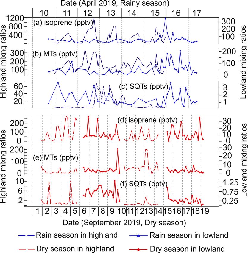
Y. Liu et al.: Seasonal and diurnal variations in biogenic volatile organic compounds                                              14763

Figure 1. Atmospheric oxidation and abiotic effects on biogenic volatile organic compounds (BVOCs) in African highland and lowland
ecosystems. The ecosystem impacts on CO2 concentration (e.g., photosynthesis and respiration) are not shown in the figure above. SOA is
secondary organic aerosol, and OH is hydroxyl radical. The green arrows indicate BVOC sources from African ecosystems. BVOC oxidation
and products are shown as purple arrows. The dashed yellow and purple arrows mean BVOC indirect impact to the climate. The abiotic effects
on BVOC emissions are shown as red arrows. Blue arrows mean rivers and groundwater. The environments of our study areas are shown
as the red house symbols. Figure courtesy of Gretchen Gettel, IHE Delft Institute for Water Education, and Yang Liu and Petri Pellikka,
University of Helsinki.

consists of dry savannas located in the lowlands, between              The annual temperature is 18.5 ◦ C at Taita Research Station
500 and 1000 m a.s.l. (above sea level), and highlands rang-           in the highlands and 22.3 ◦ C in Maktau field site in the low-
ing from approximately 1100 to 2200 m a.s.l. (Pellikka et al.,         lands between 2013 and 2021. Both meteorological measure-
2018).                                                                 ments are managed by the University of Helsinki, Finland.
   Taita Taveta County has two rainy and two dry seasons               The length of sunlight remains 12 ± 0.5 h through the en-
annually due to the Intertropical Convergence Zone forming             tire year, with sunrise around 06:00 ± 0.5 h and sunset about
a bimodal rainfall pattern. The first rainy season (often re-          18:00 ± 0.5 h depending on the season (all times are given as
ferred to as the long rains) occurs between March and June,            East Africa Time, UTC+3).
while the second rainy season (referred to as the short rains)            The experimental sites were set up in the highlands in
is between October and December. The two rainy seasons                 Wundanyi at Taita Research Station of the University of
are separated by dry seasons, with a short hot and dry sea-            Helsinki and in the lowlands in the Maktau field site to rep-
son from January to February and a long cool and dry season            resent the highland and lowland ecosystems, respectively
from June to September (Ayugi et al., 2016; Wachiye et al.,            (Fig. 2). The Taita Research Station (3◦ 400 S, 38◦ 360 E;
2020). The highlands receive more rainfall than the lowlands.          1415 m) is located in the middle of the Taita Hills on a wind-
The annual precipitation is on average 1132 mm in Mgange               ward slope. The landscape is characterized by small agricul-
(1768 m a.s.l.), corresponding to about twice the rainfall re-         tural fields with a variety of crops, such as maize, beans, av-
ceived in Voi at 560 m a.s.l. (587 mm; Erdogan et al., 2011).          ocados, and grass, with small native or exotic forest stands.

https://doi.org/10.5194/acp-21-14761-2021                                             Atmos. Chem. Phys., 21, 14761–14787, 2021
14764                                 Y. Liu et al.: Seasonal and diurnal variations in biogenic volatile organic compounds

The measurement station, which is fenced off, is surrounded
by agroforestry landscape, with the closest native and exotic
forests at 200 m distance. The natural ecosystem of the Wun-
danyi site is humid montane forest (Pellikka et al., 2009).
Broadleaf evergreen trees and lush grass covered the ground
layer during the rainy season at the Wundanyi site (Fig. 2b),
while part of the leaves were shed from trees and grass
was dried out around our instrument during the dry season
(Fig. 2c). The Maktau field site (3◦ 250 S, 32◦ 740 E; 1056 m) is
located in the lowlands in which the natural ecosystem would
be Acacia–Commiphora bushland on savanna (Amara et al.,
2020). The measurement site is located inside a fenced farm
growing maize, cassava, beans, and papaya trees, surrounded
by bushland. The soil on this site was not ploughed yet, and
the field was not sown or replanted during our rainy season
measurements (Fig. 2d). The instrument was positioned near
young cassava bush, with a distance of 50 m from the nearest
bushland edge. In the dry season, we collected the samples
2 weeks after the maize was harvested, and the dry maize
residuals still remained on the ground (Fig. 2e). The bush-
land surrounding the field was almost leafless during the dry
season sampling, while during the rainy season sampling, the
new leaves were starting to sprout. The sites were chosen
                                                                    Figure 2. Locations of the highland site (HL) in Wundanyi and the
for the following two reasons: (1) they represented typical
                                                                    lowland site (LL) in Maktau. The green color in the true color Sen-
highland agroforestry and lowland dry agriculture ecosys-           tinel satellite image (a) shows the forests and agricultural area in the
tems with typical bushland and forest cover, and (2) they pro-      Taita Hills, while magenta represents grassland with a few fire scars.
vided safety and electricity for continuous measurements.           The brownish areas are areas with less land cover, such as dry bush-
                                                                    land, dryland agriculture, and areas used for livestock management.
2.2   Sample collection and chemical analysis of BVOC               Photographs in panels (b, c, d, e) show the phenological conditions
      mixing ratios                                                 and the surrounding environments of the measurement sites during
                                                                    sampling in the rainy season in April and dry season in September.
We conducted four campaigns, each lasting several days, in          Photographs by Simon Schallhart, Finnish Meteorological Institute,
the highlands and lowlands during the onset of the hot and          and Petri Pellikka, University of Helsinki.
long rainy season from 10 to 17 April 2019 and during the
cool and long dry season from 1 to 19 September 2019 (Ta-
ble A1).                                                            (at approximately −15◦ ) after collection (for 1 to 2 weeks)
   The measurements took place upwind of the two sites,             and before analysis (about 2 months). Tubes were stored in a
away from roads and at least 10 m away from the near-               closed box, with ambient temperature and dark inside, during
est residential buildings. In total, two autosamplers were          the transportation to the Finnish Meteorology Institute (less
used to collect air into thermal desorption sorbent tubes           than 1 week).
(STS 25; PerkinElmer, Waltham, MA, USA), with a flow                   The mixing ratios of isoprene (C5 H8 ), MBO (C5 H10 O),
rate of 100 cm−3 min−1 . All tubes were filled with Tenax           MTs (C10 H16 and C10 H18 O), SQTs (C15 H24 ), and bornyl ac-
TA (60–80 mesh; Sigma-Aldrich, St. Louis, MO, USA) and              etate (C12 H20 O) were measured. MTs consisted of α-pinene,
Carbopack B (60–80 mesh; Sigma-Aldrich, St. Louis, MO,              β-pinene, limonene, 31-carene, ρ-cymene, camphene, ter-
USA). Although the cartridges were stored in an ambient             pinolene, linalool, and 1,8-cineol. SQTs consisted of longi-
temperature during sampling, sorbents used in the tubes were        cyclene, iso-longifolene, β-caryophyllene, β-farnesene, and
hydrophobic, and therefore, water was not accumulated. In           α-humulene. All samples were analyzed in the laboratory
addition, tubes were flushed with helium for 5 min with the         of the Finnish Meteorological Institute. An automatic ther-
flow of 50 mL min−1 before desorption and analysis to re-           mal desorption device (PerkinElmer TurboMatrix 650) was
move traces of humidity.                                            connected to a gas chromatograph (PerkinElmer Clarus 600)
   The sampling time was generally 4 h but was only 2 h dur-        with a DB–5MS column (50 m × 0.25 mm, film 0.5 µm) and
ing the second campaign due to frequent power failures (Ta-         a mass-selective detector (PerkinElmer Clarus 600T). We
ble A1). The sampling took place 25 cm above the ground so          desorbed all sample tubes at 300 ◦ C for 5 min before cryo-
that flowing water during heavy rainfall events did not dis-        focusing the samples in a Tenax TA cold trap (−30 ◦ C) and
turb the measurements. All samples were stored in the freezer       injecting them into the column by rapidly heating the cold

Atmos. Chem. Phys., 21, 14761–14787, 2021                                             https://doi.org/10.5194/acp-21-14761-2021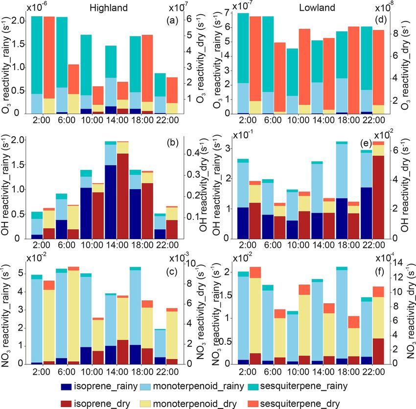
Y. Liu et al.: Seasonal and diurnal variations in biogenic volatile organic compounds                                     14765

trap to 300 ◦ C. The method, including potential losses, has     method is described at Ozonesonde, 2021) and ultraviolet B
been described in detail in Helin et al. (2020). The analyti-    (UVB) radiation intensity to calculate OH radical proxies,
cal uncertainties and the limit of quantification are shown in   using Eq. (1) (Rohrer and Berresheim, 2006; Petäjä et al.,
Table A2.                                                        2009).
   Standards in methanol solutions were used to calibrate the
MBO, MTs, and SQTs. We injected the standards into the           OHproxy = 5.62 × 10⁵ × UVB0.62 .                            (1)
sampling tubes and flushed away the methanol for 10 min be-      The calculated average midday (local noon time) concentra-
fore the analysis. The gaseous calibration standard (National    tions of O3 were 31 and 29 ppbv (parts per billion by volume)
Physical Laboratory) was applied for isoprene. Calibration       in the rainy and dry seasons, respectively, while the corre-
samples were analyzed together with real samples.                sponding concentration of OH was estimated to be 1.2 × 10⁶
                                                                 and 1.1 × 10⁶ molec. cm−3 in the rainy and dry seasons in
2.3     Complementary measurements and oxidant                   our study area, respectively.
        estimation
                                                                 2.4   Reactivity calculation
2.3.1    Meteorological data
                                                                 Calculating the reactivity of BVOCs gives insight into the
Meteorological data were measured simultaneously with            relative role of BVOCs in local atmospheric chemistry. The
sampling of BVOCs at Taita Research Station and Maktau           reactivity of BVOCs (Ri,x , where i refers to the BVOC
Weather Station. Hourly air temperature (CS215, Campbell         species and x the oxidant species) was calculated by mul-
Scientific, UK), relative humidity (CS215, Campbell Scien-       tiplying the mixing ratio of a specific BVOC (i) with the
tific, UK), precipitation (ARG100, EML, UK), wind speed,         corresponding reaction rate coefficient (ki,x ) of oxidants (in-
and direction (Taita – wind monitor 05103, R. M. Young           cluding O3 , OH, and NO3 ) using Eq. (2).
, Traverse City, MI, USA; Maktau – 03002-L wind sentry           Ri,x = BVOCi × ki,x .                                       (2)
set, R. M. Young, Traverse City, MI, USA) were measured
at both stations. All instruments were positioned at 1.5 m       The parameter ki,x was calculated by using the average air
above the ground. Atmospheric pressure (CS106 baromet-           temperature during each measurement (calculation equations
ric pressure sensor, Vaisala, Finland), photosynthetic pho-      described in Table A3). All of the reaction rate coefficients
ton flux density (PPFD; SKP215 PAR Quantum, Skye In-             used in this study are provided in Table A4.
struments, UK), and soil moisture (CS650 sensor, Campbell           The atmospheric lifetime (τ ) of different BVOCs shows
Scientific, UK) were additionally measured at Maktau. The        the oxidation speed of a specific compound or compound
PPFD sensor was positioned around 4 m above the ground.          group in the atmosphere (Eq. 3). We calculated the lifetime
Soil moisture was measured at depths of 10 and 30 cm. Root       of measured BVOCs in relation to O3 and OH (x), as stated
zone soil moisture calculation has been described in Räsänen     in Table A4.
et al. (2020).                                                          1X                         −1
    The Chemistry Land–surface Atmosphere Soil Slab              τi,x =        m
                                                                                 ki,x × Oxidantx       .                     (3)
                                                                        m
(CLASS) model was used to estimate mixing layer heights
(MLHs) at the lowland site (Python version; Vilà-Guerau de       The amount of measurements in a certain period (m) was
Arellano et al., 2015). The model initial conditions were de-    used to average over different measurement periods, de-
rived from the weather station observations. The sensible and    scribed hereafter as late night (00:00 to 04:00), early morning
latent fluxes from eddy covariance measurements were used        (04:00 to 08:00), late morning (08:00 to 12:00), early after-
as model input. These flux measurements were corrected by        noon (12:00 to 16:00), late afternoon (16:00 to 20:00), and
conserving the Bowen ratio using the net radiation measure-      early night (20:00 to 00:00).
ments (Combe et al., 2015). The diurnal MLH data start from
                                                                 2.5   Emission factor estimation
06:00 and continue to 18:00, and the MLHs ranged from
337 ± 25 to 2539 ± 197 m during the rainy season campaign        EFs were estimated for isoprene, MBO, and the detected
in April and from 361 ± 18 to 2755 ± 146 m during the dry        MTs using inverse modeling. In practice, a simple BVOC
season campaign in September. All meteorology data during        emissions and chemistry model was developed for this pur-
BVOC measurements are shown in Fig. 3.                           pose. The model includes an emissions module based on
                                                                 Guenther et al. (2012). The emissions (Fi ) of BVOCs (i) are
2.3.2    Oxidant concentration estimation                        calculated as Eq. (4) as follows:

Since the concentrations of oxidants were not measured di-       Fi = γi · EFi ,                                             (4)
rectly during the campaigns, we used data observed by an         where
Ozone Monitoring Instrument to acquire O3 column densi-
ties to estimate surface O3 concentrations (the conversion       γi = CCE LAIγp,i γT ,i γSM .

https://doi.org/10.5194/acp-21-14761-2021                                          Atmos. Chem. Phys., 21, 14761–14787, 2021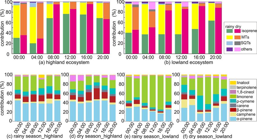
14766 Y. Liu et al.: Seasonal and diurnal variations in biogenic volatile organic compounds
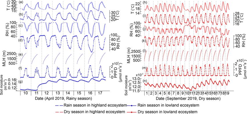
Figure 3. Meteorological measurements in the highland (H) and lowland (L) ecosystems during the rainy and dry seasons. PPFD is photo-
synthetic photon flux density.
The γi is an activity factor which accounts for emission re- where
sponses due to various environmental parameters and pheno-
Eopt = Ceo,i × exp (0.05 × (T24 − Ts ))
logical conditions. We considered BVOC emission responses
due to light (γp,i ; Eq. 5), temperature (γT ,i ; Eq. 6), and × exp (0.05 × (T240 − Ts ))
soil moisture (γSM ; Eq. 7). A value of 0.57 was assigned
1 1
to the canopy environment coefficient (CCE ; Simpson et al., x= − /0.00831.
313 + (0.6 × (T240 − Ts )) T
1999, 2012; Guenther et al., 2012), while the one–sided
leaf area index (LAI, 2020) was kept constant at a value of Ceo,i is an emission-class-dependent empirical coefficient for
1.53 m2 m−2 (April) or 0.3 m2 m−2 (September). each BVOC in Table 4 in Guenther et al. (2012). Ts rep-
resents the standard conditions for leaf temperature and is
equal to 297 K. T24 and T240 are the average leaf tempera-
γp,i = (1 − LDFi ) + LDFi ture of the past 24 h and the past 240 h, respectively. The leaf
0.5
2 2 temperatures were calculated from observed air temperatures
× Cp (α × PPFD) / 1 + α × PPFD , (5)
(Eqs. 14.2 to 14.6 in Campbell and Norman, 1998). βi , CT 1,i ,
and CT 2 are the empirically determined coefficients. We used
230 for CT 2 , according to Guenther et al. (2012), and values
where
for βi and CT 1,i from Table 4 in Guenther et al. (2012).
Cp = 0.0468 × exp (0.0005 × [P24 − Ps ]) × [P240 ]0.6 1 θ > θl
θ −θw
γSM, isoprene = θw < θ < θl , (7)
α = 0.004 − 0.0005 ln (P240 ) . 1θl
0 θ < θw
The parameter LDFi is the light-dependent fraction of the where θ is the volumetric water content of soil. θl = θw +
emission of each individual BVOC, and the values are pro- 1θl , θw is the wilting point and was set to 0.1 m3 m−3 for the
vided in Guenther et al. (2012). Ps is the standard condi- Maktau site (Räsänen et al., 2020), while 1θl is an empirical
tion for PPFD, averaged over the past 24 h, and was set to parameter which equals 0.04 (Guenther et al., 2012). γSM is
200 µmol m−2 s−1 (Guenther et al., 2012). P24 and P240 are only applied for the estimation of the emission of isoprene,
the average PPFD of the past 24 h and the past 240 h, respec- according to Guenther et al. (2012).
tively. The model’s chemistry module consists of the first step in
the oxidation of the BVOCs by O3 and OH using the reac-
tion rate coefficients listed in Table A3. Reactions with NO3
γT ,i = (1 − LDFi ) × exp (βi (T − Ts )) + LDFi × Eopt were omitted because simulations were only carried out us-
exp (CT 1 × x) ing daytime observations. The model takes the following pa-
× CT 2 × , (6) rameters as input: observations of PPFD, air temperature, soil
CT 2 − CT 1 × (1 − exp (CT 2 × x))
Atmos. Chem. Phys., 21, 14761–14787, 2021 https://doi.org/10.5194/acp-21-14761-2021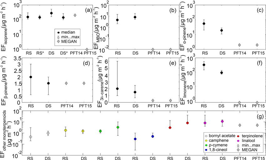
Y. Liu et al.: Seasonal and diurnal variations in biogenic volatile organic compounds                                     14767

moisture from the Maktau site, estimated leaf temperatures,       in the rainy season were higher than in the dry season in both
estimated concentrations of O3 and OH (Sect. 2.3.2), mod-         the highlands and lowlands. The seasonal mean ± standard
eled daytime MLHs (Sect. 2.3.1), and LAI. In the model, the       deviation of the isoprene mixing ratio was 252.2 ± 285 and
concentration of O3 is kept constant within a day, while the      66.6 ± 75 pptv in the highlands in the rainy and the dry
daily pattern of the OH concentration follows the solar zenith    season, respectively, while the corresponding values were
angle.                                                            145.5 ± 73 and 35.2 ± 42 pptv for MTs (Fig. 4). In the
   Initial estimations were made for the EFs, and the mixing      lowlands, the mixing ratio of isoprene was 55.3 ± 56 and
ratios of the BVOCs were predicted using the model for 1          11.2 ± 9 pptv in the rainy and the dry season, respectively,
campaign day at a time. The predicted and measured daytime        while the corresponding values for MTs were 57.8 ± 46 and
BVOC mixing ratios were then compared (2–5 data points            4.1 ± 4 pptv. Isoprene and all the MTs showed a clear mixing
per day), and the sum of the squared differences between the      ratio maximum in the rainy season, and the seasonal mixing
predicted and observed mixing ratios was calculated for each      ratios of isoprene and MTs remained lower in the lowlands
individual BVOC for each day. A new estimation for the val-       than in the highlands. The temporal variability in measured
ues of the EFs was made, and the process was iterated until a     BVOCs is presented in Fig. A3.
minimum sum of the squared differences was obtained (Ta-             Significantly higher temperature, more emitters from dif-
ble A5). The EF, for each individual BVOC, which led to this      ferent vegetation types, and the lower mixing layer heights
minimum value, was considered the most appropriate value          were probably the main factors promoting higher mixing ra-
for the EF for that particular day (Table A5). Similar simu-      tio during the rainy season (Fig. A4; Table 1). Soil moisture
lations were conducted for each measured day. The median          was additionally so low during the dry season (Fig. A5g, h)
values of the estimated EFs during either the rainy or dry        that it has most probably reduced the emission rate of iso-
season, for each individual BVOC, are our best estimates for      prene. PPFD, RH, and estimated atmospheric oxidant con-
the BVOC EFs for the agriculture site located in the savanna      centrations stayed largely the same during the two seasons
ecosystem at Maktau field site. A comparison of the mod-          and, thus, did not influence the concentration difference. The
eled and measured BVOC concentrations, which lead to the          slightly different PPFD between the two seasons should not
minimum sums of the squared differences between the pre-          have impacted the emission of isoprene, since the light condi-
dicted and observed mixing ratios, is provided in Figs. A1        tions during both seasons were still higher than the saturation
and A2. Similar estimations of EFs were not conducted for         point for the production and emission of isoprene (Fig. A5f,
the highland site, due to lack of necessary input data to the     m; Guenther et al., 2006). It is likely that the significantly
model.                                                            higher LAI in the highlands also caused higher BVOC mix-
                                                                  ing ratios in the highlands compared to the lowlands. Addi-
                                                                  tionally, the vegetation type in the two ecosystems are dif-
3     Results and discussion                                      ferent, which might also contribute to the difference, though
                                                                  in which direction is unclear, since emission rates from the
3.1     Seasonal and diurnal variations of BVOC mixing
                                                                  particular plant species populating the areas have not been
        ratios
                                                                  reported so far to our knowledge.
For most of the compounds studied, the daily mean mix-               The mixing ratio of isoprene showed distinct diurnal vari-
ing ratio was higher during the rainy season than during the      ation in the highlands during both the rainy and dry seasons
dry season. In the highlands, the daily mean isoprene mix-        but in the lowlands only during the dry season (Figs. A6 to
ing ratio ranged from 134 to 442 pptv in the rainy season and     A9). The mixing ratio of isoprene increased in the morning,
ranged from 36 to 150 pptv in the dry season. The daily mean      coinciding with sunrise, and stayed high during the rest of
mixing ratio of MTs was 117 to 233 pptv in the rainy season       the day. The measured mixing ratio of isoprene contributed
and was 8 to 75 pptv in the dry season. And that of SQTs          on average 37 % and 84 % in the highlands and lowlands, re-
was 2 to 30 pptv in the rainy season and 1 to 3 pptv in the       spectively, to the total BVOC mixing ratio (Fig. 5).
dry season. In the lowlands, the daily mean mixing ratios of         The mixing ratios of MTs showed higher mixing ratios
isoprene ranged from 22 to 69 pptv and from 6 to 15 pptv in       during night and dark hours than during light hours, particu-
the rainy and the dry season, respectively. The mixing ratio      larly during the dry season in both ecosystems (Figs. A6 to
of MTs was from 29 to 96 pptv in the rainy season and from        A9). Higher mixing ratios of MTs during the night have been
3 to 9 pptv in the dry season. For SQTs, the daily mean mix-      observed earlier in savannas in South Africa (Gierens et al.,
ing ratios ranged from 1 to 2 pptv and was less than 1 pptv in    2014), and a needleleaf forest in California, USA, and Fin-
the rainy and the dry season, respectively.                       land (Bouvier-Brown et al., 2009; Hakola et al., 2012). Even
                                                                  though the MT emissions are expected to be highest during
3.1.1    Mixing ratios of isoprene and monoterpenoids             daytime, the mixing ratio of MTs is lower since the mixing,
                                                                  and therefore dilution, is highest during daytime and lowest
Isoprene and MTs explained over 88 % of the total BVOC            during the night (Mogensen et al., 2011; Hellén et al., 2018).
mixing ratios of all collected samples, and their mixing ratios

https://doi.org/10.5194/acp-21-14761-2021                                       Atmos. Chem. Phys., 21, 14761–14787, 2021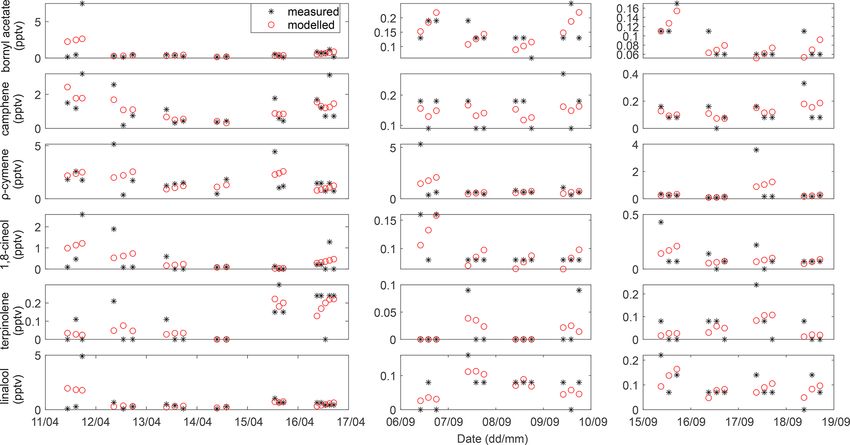
14768                                         Y. Liu et al.: Seasonal and diurnal variations in biogenic volatile organic compounds

Figure 4. Mixing ratios of isoprene, monoterpenoids, sesquiterpenes, and others (2-Methyl-3-buten-2-ol and bornyl acetate) in the highland
and lowland ecosystems during the rainy and dry seasons.

Table 1. LAI, the concentration of ozone, and meteorology conditions detected or estimated in the highland and the lowland sites during the
campaigns. Parameters which were not measured in situ are indicated.

               Season       Site               LAIa           Tb        c
                                                                      TDt             PPFDdDt          RHe       MLHfDt            SMg            Oh3
                                           (m2 m−2 )          (◦ )     (◦ )    (µmol m−2 s−1 )         (%)         (m)         (m3 m−3 )        (ppb)
               Rainy        Highland              2.08      20.9     22.7                     nan       87.3          nan              nan       30.9
                            Lowland               1.53      23.9     25.5                   867.7       75.1        663.9             0.15       31.2
               Dry          Highland                1.9     17.3     18.6                     nan       86.8          nan              nan       28.6
                            Lowland                 0.3     20.5     22.2                   865.5       75.0        819.6             0.12       28.8
             a LAI – leaf area index (from satellite); b T – daily mean ambient temperature; c T – average of daytime (06:00 to 18:00) ambient
                                                                                                Dt
             temperature; d PPFDDt – daytime mean photosynthetic photon flux density; e RH – daily mean relative humidity; f MLHDt – average of
             daytime mean mixing layer height (estimated); g SM – daily mean soil moisture; h O3 – estimated daily mean concentration of ozone; nan – no
             observations available; ppb – parts per billion.

   The diurnal maximum mixing ratio of MTs was on average                             (Greenberg et al., 1999). In western Africa, isoprene mix-
254 and 56 pptv in the highlands and 89 and 11.5 pptv in the                          ing ratios of over 1000 pptv during daylight hours were mea-
lowlands in the rainy and the dry seasons, respectively. The                          sured in a forest surrounded by a woodland savanna ecosys-
diurnal variations in α-pinene and limonene controlled the                            tem in Benin (Saxton et al., 2007). The western African
changes in total MT mixing ratio and contributed over 60 %                            and the two central African measurements aforementioned
to the total MT mixing ratio. Decreasing mixing ratios of                             all showed at least an order of magnitude higher isoprene
limonene between day and night led to the diurnal variation                           mixing ratios compared with the measurements in the high-
in the total mixing ratio of MTs in the rainy season, while                           lands (Wundanyi) of this study (Table 2). The measured mix-
decreasing α-pinene controlled the diurnal variation in total                         ing ratios of α-pinene, limonene, and β-pinene in Wundanyi
MTs in the dry season. The minimum diurnal mixing ratio of                            were comparable to the corresponding compound levels from
MTs occurred in the early night during the rainy season and                           the aforementioned forest measurements. The mixing ratios
around noon in the dry season.                                                        of isoprene and MTs in Wundanyi are comparable to our
   The isoprene mixing ratio ranged from 730 to 1820 pptv                             previous measurements from three types of montane native
in the rainy season of 1996 in a tropical forest in the north-                        forests of the Taita Hills in southern Kenya (Liu et al., 2021).
ern Republic of the Congo (RC), which was covered by ev-                              The mixing ratios of isoprene and MTs at the lowland site
ergreen or semi-evergreen trees (Serça et al., 2001). A sim-                          in Maktau were about 4 times lower than the correspond-
ilar level of isoprene mixing ratio was observed in a forest                          ing levels measured from savanna ecosystems in the Cen-
ecosystem near Enyele, northern RC, with values ranging                               tral African Republic (Boali) and South Africa (Greenberg
from 700 to 1000 pptv at the end of the rainy season of 1996                          et al., 1999; Harley et al., 2003) and grass and shrubland in

Atmos. Chem. Phys., 21, 14761–14787, 2021                                                                   https://doi.org/10.5194/acp-21-14761-2021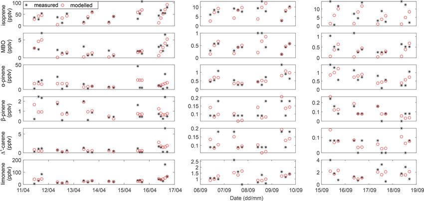
Y. Liu et al.: Seasonal and diurnal variations in biogenic volatile organic compounds                                             14769

Figure 5. Diurnal contribution of biogenic volatile organic compounds (a, b) and contribution of monoterpenoids (MTs) (c, d, e, f) across
the highland site and the lowland site in the rainy and the dry seasons. SQTs is sesquiterpenes, and others are 2-Methyl-3-buten-2-ol and
bornyl acetate.

western Senegal (Grant et al., 2008) and considerably lower            contribution to the local atmospheric chemistry can still be
than the corresponding compound levels from woodland in                significant. The highest daily means were measured during
Botswana (Greenberg et al., 2003). The mixing ratios of iso-           the nighttime, which was the same as in the case of the MTs.
prene and limonene in the rainy season in Maktau are higher            β-caryophyllene showed the highest mixing ratios among
than the levels of the corresponding compounds in grassland            the SQTs, followed by β-farnesene and/or α-humulene mea-
in Welgegund, South Africa, while the mixing ratios of α-              sured in both the rainy and dry seasons. The diurnal trend of
pinene and β-pinene, both in the rainy and the dry seasons, as         β-caryophyllene and β-farnesene followed the variation in
well as isoprene and limonene in the dry season in Maktau,             total SQTs.
were lower than the values reported by Jaars et al. (2016).               The mixing ratios of MBO and bornyl acetate were both
The mixing ratios of α-pinene, limonene, and β-pinene in               low. MBO explained 2.6 % of the total BVOC mixing ratio
the rainy season in Maktau were all in the range of the mix-           of all samples, while bornyl acetate explained 0.5 %. Both
ing ratios of the corresponding compounds in our previous              compounds have seasonal and diurnal variations. The sea-
measurements, while that of isoprene was at lower levels               sonal mean mixing ratios of MBO and bornyl acetate were
than previously reported (Liu et al., 2021). The differences           5 and 1.5 times higher in the rainy season than in the dry
in mixing ratios between our measurement and from these                season in the highlands, respectively, and the mixing ratios
aforementioned studies could be affected by several factors,           of both BVOCs were 6 times higher in the lowlands. The di-
e.g., dominant plant species and their distribution, tempera-          urnal mean mixing ratios of MBO and bornyl acetate were
ture and light, wind speed/direction, mixing layer height, etc.        around 4 and 0.8 pptv in the rainy season in both the high-
But we were not able to find the key reasons based on the              lands and lowlands. MBO mixing ratios were 1 and 0.7 pptv
limited details from the other sites.                                  in the dry season in the highlands and lowlands, while that of
                                                                       bornyl acetate was 0.6 and 0.1 pptv, respectively. The daily
3.1.2   Mixing ratios of sesquiterpenes, MBO, and                      mean mixing ratio of bornyl acetate was lower than 1 pptv in
        bornyl acetate                                                 the rainy and dry seasons both in the highlands and lowlands.
                                                                          Jaars et al. (2016) measured MBO for the first time in
The mixing ratios of SQTs were low and contributed to                  Africa, and they reported that the mean mixing ratios of
around 3 % of the total BVOC mixing ratios in all sam-                 MBO were 12 and 8 pptv in their first and second cam-
ples. SQTs showed seasonal and diurnal variations similar              paign, respectively, which are higher than the mean MBO
to those of MTs, but their mixing ratio was much lower                 mixing ratios measured in the highlands and lowlands in this
than that of MTs, with seasonal mean SQT mixing ratios of              study. Guenther (2013) stated that MBO is emitted from most
15.0 ± 19 and 1.1 ± 2 pptv in the highlands and 1.5 ± 0.9 and          isoprene-emitting vegetation at an emission rate of ∼ 1 % of
0.5 ± 0.3 pptv in the lowlands in the rainy and the dry sea-           that of isoprene. The Welgegund data (Jaars et al., 2016)
sons, respectively. SQTs are very reactive, and therefore their        showed that MBO is approximately 30 % of the isoprene

https://doi.org/10.5194/acp-21-14761-2021                                             Atmos. Chem. Phys., 21, 14761–14787, 2021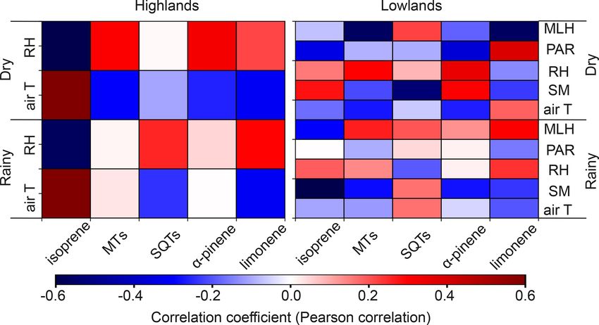
14770                                  Y. Liu et al.: Seasonal and diurnal variations in biogenic volatile organic compounds

Table 2. Mixing ratios of biogenic volatile organic compounds in different ecosystems in Africa (mixing ratios are presented as median and
mean values, except those with extra explanations (e.g., midday, minimum/maximum, and mean ± SD. The unit of mixing ratios is presented
in pptv).

    Location                  Time                      Vegetation                    Compound      Mixing ratio         Reference
                                                                                                    median (mean)
    Wundanyi, Kenya           April and September       Agroforestry                  Isoprene      Rainy: 78 (252)      This study
    (38.4◦ E, 3.4◦ S)         2019                                                                  Dry: 34 (66)
                                                                                      α-Pinene      Rainy: 54 (59)
                                                                                                    Dry: 12 (15)
                                                                                      Limonene      Rainy: 37 (42)
                                                                                                    Dry: 3.4 (6.4)
                                                                                      β-Pinene      Rainy: 13 (15)
                                                                                                    Dry: 3.9 (4.7)
    Maktau, Kenya                                       Savanna bushland              Isoprene      Rainy: 43 (55)
    (32.7◦ E, 3.3◦ S)                                                                               Dry: 8.7 (11)
                                                                                      α-Pinene      Rainy: 8.0 (14)
                                                                                                    Dry: 0.7 (1.1)
                                                                                      Limonene      Rainy: 27 (34)
                                                                                                    Dry: 1.0 (1.2)
                                                                                      β-Pinene      Rainy: 1.6 (2.5)
                                                                                                    Dry: 0.2 (0.3)
    Enyele, RC                November and              Forest                        Isoprene      700 to 1000          Greenberg
    (18◦ E, 3◦ N)             December 1996                                                                              et al. (1999)
                                                                                      α-Pinene      30 to 100
    Boali, Central African                              Savanna                       Isoprene      100 to 400
    Republic
    (18◦ E, 4.5◦ N)
                                                                                      α-Pinene      20 to 30
    Northern RC               March 1996                Tropical evergreen forest;    Isoprene      Mean ± SD:           Serça et al.
    (16.2◦ E, 2.1◦ S)                                   semi-evergreen forest                       1820 ± 870           (2001)
                              November 1996                                           Isoprene      Mean ± SD:
                                                                                                    730 ± 480
                              March and                                               β-Pinene      < 10
                              November 1996
    South Africa              February 2001             Combretum–Acacia              Isoprene      Midday 390           Harley et
    (29.8◦ E, 25.0◦ S)                                  savanna                                                          al. (2003)
    Botswana                  February 2001             Mopane woodland               α-Pinene      Minimum              Greenberg
    (23.3◦ E, 19.5◦ S)                                                                              < 1000               et al. (2003)
                                                                                                    Maximum
                                                                                                    > 2000
    Benin                     June 2006                 Forest                        Isoprene      Day_maximum          Saxton et
    (1.4◦ E, 9.4◦ N)                                                                                > 1000               al. (2007)
                                                                                                    Night_maximum
                                                                                                    > 500
                                                                                      Limonene      Few tens to 5000

Atmos. Chem. Phys., 21, 14761–14787, 2021                                                https://doi.org/10.5194/acp-21-14761-2021
Y. Liu et al.: Seasonal and diurnal variations in biogenic volatile organic compounds 14771
Table 2. Continued.
Location Time Vegetation Compound Mixing ratio Reference
median (mean)
Republic of Senegal September 2006 Grasses; shrubs Isoprene Minimum 200; Grant et al.
(17.1◦ W 14.7◦ N) maximum 400 (2008)
Benin 17 August 2006 Subtropical forest Isoprene Midday 1184 Stone et al.
(2.7◦ E, 10.1◦ N) mean ± SD: (2010)
294 ± 333
Welgegund, February 2011 to Grassland Isoprene First: 14 (28); Jaars et al.
South Africa February 2012 (first); second: 14 (23) (2016)
(26.9◦ E, 26.6◦ S) December 2013 to
February 2015
(second)
α-Pinene First: 37 (71);
second: 15 (57)
Limonene First: 21 (30);
second: 16 (54)
β-Pinene First: 9 (19);
second: 3 (5)
Kenya April 2019 Montane forest Isoprene 741 (706) Liu et al.
(32–38◦ E, 3.2–3.4◦ S) (2021)
α-Pinene 74 (75)
Limonene 6.6 (7.7)
β-Pinene 7.2 (7.9)
Grass and shrubs Isoprene 735 (713)
α-Pinene 30 (25)
Limonene 50 (56)
β-Pinene 5.3 (4.6)
mixing ratio, and thus, their study indicated that MBO at activity of SQTs was 5 to 30 times higher than for other
Welgegund is most likely from other MBO-emitting species BVOCs, with β-caryophyllene having the highest contribu-
than from isoprene emitters. MBO are higher than 1 % of iso- tion to the total O3 reactivity. The strong relative importance
prene mixing ratios in our study, which was 3.7 % and 6.3 % of the SQTs compared with other BVOCs for the local O3
of the isoprene mixing ratio in the highlands in the rainy and reactivity has also been seen in the ambient air of a Scots
dry seasons, respectively, and 7.6 % and 9.8 % in the low- pine forest in Finland (Hellén et al., 2018). Out of the to-
lands. Unfortunately, we could not partition the source of tal BVOCs, MTs contributed most to the NO3 reactivity, an
MBO emitter(s) in this study area during our measurements. average of 13 and 15 times more than isoprene and SQTs,
Be aware that no measurements were conducted during the respectively. MTs also contributed to the OH reactivity, with
short hot (January to February) and short cool (October to a 0.7 to 1.9 times higher contribution than isoprene during
December) season, and it is likely that the mixing ratios of nighttime, while isoprene is the dominant BVOC contribu-
BVOCs are different during those seasons than what is pre- tor to the OH reactivity during the day, with 3.1 to 3.5 times
sented here due to differences in, e.g., environmental condi- higher contributions than MTs.
tions and phenology status. Isoprene shows the highest mixing ratio of BVOCs in this
study. The atmospheric lifetime of isoprene is 34 and 2.3 h
3.2 Reactivity of the measured BVOCs with oxidants with O3 and OH, respectively. Following that of isoprene,
limonene (∼ 2 h) and α-pinene (∼ 4 h) have higher mixing
The reactivity toward O3 , OH, and NO3 was calculated us- ratios and are detected to have a relatively short lifetime with
ing the measured BVOC mixing ratios (Fig. 6). The O3 re- OH and O3 compared with other MTs (except terpinolene
https://doi.org/10.5194/acp-21-14761-2021 Atmos. Chem. Phys., 21, 14761–14787, 202114772 Y. Liu et al.: Seasonal and diurnal variations in biogenic volatile organic compounds
and linalool). A higher importance of limonene and α-pinene β-pinene, and 31-carene compared with the EFs for other
for OH reactivity than other MTs was also observed in a sa- plant functional types in MEGAN. However, the estimated
vanna ecosystem in South Africa (Jaars et al., 2016), which EF for limonene is more in line with MEGAN’s EF for trop-
reported that both compounds also had higher mixing ratios ical trees (80 µg m−2 h−1 ). Unfortunately, we could not iden-
than other MTs during their campaigns. Compared with other tify the source of the limonene emitter(s). It could be the
MTs, limonene has a significantly higher yield for highly native African shrubs surrounding the lowland site, which
oxygenated organic molecules (Ehn et al., 2014; Bianchi et are dominated by acacias (Senegalia mellifera; Vachellia tor-
al., 2019), which has been found to be a major component of tilis), but to our knowledge, emission rates have not been re-
secondary organic aerosols (e.g., Ehn et al., 2014; Mutzel et ported from these species. The EF for the sum of other MTs
al., 2015), for which higher limonene is expected to have a (i.e., six MTs at our site and up to 34 in MEGAN) is about
strong impact on local aerosol production in southern Kenya 10 and 20 µg m−2 h−1 higher than that assumed in MEGAN
as well. The low mixing ratios of β-caryophyllene and α- for warm C4 grass and Crop1 for the rainy and dry seasons,
humulene have shorter lifetimes with OH and O3 than other respectively (Fig. 7g). During both seasons, linalool con-
SQTs and BVOCs. The lifetimes of β-caryophyllene and α- tributes the most to the total EF for the sum of other MTs in
humulene are a few minutes with O3 and about 1 h with OH this study, while terpinolene accounts for the second-largest
(Table A4). fraction. Since the lifetime of monoterpenes is a few hours
(see Sect. 3.2), it is likely that part of the detected monoter-
3.3 Estimation of BVOC emission factors penes have been transported to the site from areas covered by
other plant functional types than warm C4 grass and Crop1,
The EFs for isoprene, MBO, and detected MTs, for the agri- such as broadleaved trees and shrubs, which are thought to
culture savanna ecosystem surrounding the Maktau site, were have a significantly higher potential to emit monoterpenes
estimated for the rainy and dry seasons separately (Fig. 7). (Guenther et al., 2012). It is, however, noteworthy that our
The median values of the EF for α-pinene, β-pinene, 31- estimated EF for β-pinene is in line with the listed value by
carene, camphene, and limonene (Fig. 7c to g) are higher Guenther et al. (2012) for warm C4 grass and Crop1, but not
during the rainy season in April than during the dry season for broadleaved trees and shrubs, though the lifetime of β-
in September, while the median values of the EF for MBO pinene is within the same range as that of the other monoter-
(Fig. 7b) and all other MTs (Fig. 7g) are higher during the penes. The estimated EF for MBO is much higher than that
dry season than during the rainy season. If the dependency of used for C4 grass in MEGAN. MBO has a lifetime of about
soil moisture availability on the emission of isoprene is con- half a day, and thus a great part of the detected MBO does not
sidered, then the EF for isoprene during both the rainy and originate from the near vicinity of the site but can have been
dry seasons is effectively the same (Fig. 7a). Considering the transported far distances. However, the EF listed in Guenther
variability in the estimated EFs for the two different seasons, et al. (2012) for MBO for all plant functional types present in
only the EFs for limonene show no overlap in the indicated the relevant parts of Africa (Ke et al., 2012) is still about 2–3
error bars (Fig. 7f), which are defined by the minimum and orders of magnitude lower than estimated here. This might
maximum daily estimated EF. Thus, our results suggest that call for a revision of EFs for MBO, considering that Jaars
the EF for limonene might be seasonally dependent. et al. (2016) also found even higher concentrations of MBO
In order to put the estimated EFs into context and to than we did in this study in an area of Africa which also
contribute to an improved representation of BVOC emis- should not contain MBO-emitting species.
sions from African ecosystems in models, the estimated We emphasize that the estimated EFs are connected with a
EFs are compared with the EFs used in MEGAN v2.1 for large degree of uncertainty, since they are not based on flux
warm C4 grass and Crop1 (Guenther et al., 2012). The measurements from the site but are instead determined us-
estimated EFs for isoprene (155 µg m−2 h−1 in the rainy ing observed BVOC mixing ratios and an inverse modeling
season; 280 µg m−2 h−1 in the dry season) and β-pinene approach, which is limited by model assumptions and inputs.
(2 µg m−2 h−1 in the rainy season; 1.5 µg m−2 h−1 in the dry
season) compare very well with the EFs used in MEGAN
for warm C4 grass (Fig. 7a, d) and, in the case of β-pinene, 4 Conclusion
also for Crop1, since MEGAN assumes the same EF for
β-pinene for the two different plant functional types. The In this study we measured mixing ratios of isoprene, MTs,
estimated median EFs for MBO, α-pinene, 31-carene, and SQTs, bornyl acetate, and MBO in the humid highland and
limonene are higher than the EFs used in MEGAN v2.1 by dry lowland ecosystems in Taita Taveta County, southern
about 8 (4), 17 (53), 1 (2), and 89 (314) µg m−2 h−1 , respec- Kenya, during both a rainy and a dry season.
tively, where the values in parenthesis are for the rainy sea- Isoprene and MTs showed the highest mixing ratios in
son, while the others are for the dry season. The values of both the highlands and lowlands, while α-pinene, limonene,
the estimated EFs compare best with the EFs allocated for and β-pinene accounted for the largest contribution to the to-
warm C4 grass in MEGAN in the case of isoprene, α-pinene, tal mixing ratio of MTs. Isoprene dominated the total BVOC
Atmos. Chem. Phys., 21, 14761–14787, 2021 https://doi.org/10.5194/acp-21-14761-2021Y. Liu et al.: Seasonal and diurnal variations in biogenic volatile organic compounds 14773 Figure 6. Reactivity of ozone (O3 ), hydroxyl (OH), and nitrate (NO3 ) of different biogenic volatile organic compounds in the high- land (a, b, c) and lowland ecosystems (d, e, f) in the rainy and dry seasons. Figure 7. Estimated biogenic volatile organic compound (BVOC) emission factors (EFs) for the agriculture savanna ecosystem surrounding the Maktau field site in comparison with the EFs for warm C4 grass (PFT14) and Crop1 (PFT15) used in MEGAN v2.1. The EFs have been estimated for the rainy season (RS; April) and for the dry season (DS; September) separately. (a) Isoprene (the EF was estimated by either considering RS or DS or neglecting RS∗ or DS∗ , which is a dependency of the activity factor on soil moisture availability), (b) 2-Methyl-3- buten-2-ol, (c) α-pinene, (d) β-pinene, (e) 31-carene, (f) limonene, and (g) other monoterpenes, which includes the sum of up to 34 other monoterpenes in MEGAN v2.1 and includes bornyl acetate (gray), camphene (yellow), ρ-cymene (green), 1,8-cineol (blue), terpinolene (red), and linalool (magenta) at Maktau Weather Station. The legend provided in panel (a) is valid for panels (a) to (f). https://doi.org/10.5194/acp-21-14761-2021 Atmos. Chem. Phys., 21, 14761–14787, 2021
14774                                   Y. Liu et al.: Seasonal and diurnal variations in biogenic volatile organic compounds

mixing ratio during daytime and reached diurnal peak mix-
ing ratios in the afternoon in the highlands and in the early
evening in the lowlands. The mixing ratio of MTs generally
peaked between midnight and early morning, and MTs dom-
inated the total BVOC mixing ratio during nighttime. Iso-
prene was the dominant BVOC contributor to the OH reactiv-
ity, MTs dominated the NO3 reactivity of BVOCs, and SQTs
showed higher contributions to the O3 reactivity of BVOCs
than isoprene and MTs.
   Using an inverse model approach with measured BVOC
mixing ratios and meteorology data, we estimated the EFs for
isoprene, MBO, and MTs in the agriculture savanna ecosys-
tem. The estimated EFs for isoprene and β-pinene agreed
very well with what is currently assumed in MEGAN v2.1
for warm C4 grass, but the estimated EFs for MBO, α-pinene,
and especially limonene were significantly higher than what
is assumed in MEGAN for the relevant plant functional type.
Additionally, our results indicate that the EF for limonene
might be seasonally dependent.

Appendix A

Table A1. Sample and flow rate measurements at the Wundanyi station and Maktau field site during the rainy and dry season (sccm – standard
cubic centimeters per minute).

                                          Wundanyi station (humid highland)          Maktau field site (dry lowland)
                                         First campaign     Second campaign       First campaign     Second campaign
                  Rainy season (2019)    10–13 April        13–15 April           10–13 April        14–17 April
                                         4 h per tube       2 h per tube          4 h per tube       2 h per tube
                                         Total: 22 tubes    Total: 24 tubes       Total: 22 tubes    Total: 24 tubes
                                         100.5 sccm         99.5 sccm             70 sccm            67 sccm
                  Dry season (2019)      1–5 September      10–14 September       6–10 Septem-       16–19 September
                                         4 h per tube       4 h per tube          ber                4 h per tube
                                         Total: 24 tubes    Total: 24 tubes       4 h per tube       Total: 24 tubes
                                         85.5 sccm          81.5 sccm             Total: 24 tubes    92 sccm
                                                                                  83 sccm

Atmos. Chem. Phys., 21, 14761–14787, 2021                                                https://doi.org/10.5194/acp-21-14761-2021
Y. Liu et al.: Seasonal and diurnal variations in biogenic volatile organic compounds 14775
Table A2. The analytical uncertainty (U ) for ambient temperature and the limit of quantification (LOQ) for the studied compounds. The
estimation method is described in Helin et al. (2020).
Compounds U (%) LOQ (pptv)
Isoprene 20 2.5
α-Pinene 17 0.5
Camphene 17 0.1
β-Pinene 17 0.2
Limonene 17 0.9
ρ-Cymene 17 0.3
31-Carene 16 0.3
18-Cineol 18 0.4
Terpinolene 19 1.0
Linalool 20 1.2
Longicyclene 19 0.3
Iso-longifolene 20 0.4
β-Caryophyllene 18 1.0
β-Farnesene 23 2.0
α-Humulene 19 0.3
MBO 20 0.9
Bornyl acetate 21 0.5
Figure A1. Measured and modeled mixing ratios of BVOCs.
https://doi.org/10.5194/acp-21-14761-2021 Atmos. Chem. Phys., 21, 14761–14787, 202114776 Y. Liu et al.: Seasonal and diurnal variations in biogenic volatile organic compounds
Figure A2. Measured and modeled mixing ratios of BVOCs.
Figure A4. Correlation coefficients between BVOCs and environ-
mental factors.
Figure A3. The temporal variability in biogenic volatile organic
compound mixing ratios in the highland and lowland ecosystems
during the rainy and dry seasons. (a, d) Isoprene. (b, e) Monoter-
penoids (MTs). (c, f) Sesquiterpenes (SQTs).
Atmos. Chem. Phys., 21, 14761–14787, 2021 https://doi.org/10.5194/acp-21-14761-2021Table A3. Reaction rate coefficients (ki,x ) applied in the model used for estimations of the emission factors and for reactivity calculations. T (K) is air temperature.
Compound kO3 (cm3 s−1 ) Reference kOH (cm3 s−1 ) Reference
Isoprene 1.03 × 10⁻¹⁴ · e −1995
T IUPAC preferred value 2.70 × 10⁻¹¹ · e 390
T Master Chemical Mechanism, MCM v3.2 (Jenkin
(https://iupac-aeris.ipsl.fr/htdocs/datasheets/doc/ et al., 1997; Saunders et al., 2003; http://mcm.york.
Ox_VOC7_O3_CH2C(CH3)CHCH2.doc, last ac.uk/, last access: 4 October 2021)
access: 4 October 2021)
MBO 1.0 × 10⁻¹⁷ Grosjean and Grosjean (1994) 8.1 × 10⁻¹² · e 610
T Rudich et al. (1995)
Bornyl acetate – Bornyl acetate does not react with O3 because it is 13.9 × 10⁻¹² Coeur et al. (1999)
https://doi.org/10.5194/acp-21-14761-2021
a saturated hydrocarbon
α-Pinene 8.05 × 10⁻¹⁶ · e −640
T IUPAC preferred value 1.2 × 10⁻¹¹ · e 440
T IUPAC preferred value
(https://iupac-aeris.ipsl.fr/htdocs/datasheets/doc/ (https://iupac-aeris.ipsl.fr/htdocs/datasheets/doc/
Ox_VOC8_O3_apinene.doc, last access: 4 October HOx_VOC9_HO_apinene.doc, last access: 4 Octo-
2021) ber 2021)
Camphene 9.0 × 10⁻¹⁹ Atkinson (1997) 5.3 × 10⁻¹¹ Atkinson (1997)
β-Pinene 1.35 × 10⁻¹⁵ · e −1270
T IUPAC preferred value 2.38 × 10⁻¹¹ · e 357
T Kleindienst et al. (1982)
(https://iupac-aeris.ipsl.fr/htdocs/datasheets/doc/
Ox_VOC19_O3_bpinene.doc, last access: 4 Octo-
ber 2021)
31-Carene 3.7 × 10⁻¹⁷ Atkinson (1997) 8.8 × 10⁻¹¹ Atkinson (1997)
ρ-Cymene 5.0×10⁻²⁰ Hellén et al. (2018) 1.5 × 10⁻¹¹ Corchnoy and Atkinson (1990)
Y. Liu et al.: Seasonal and diurnal variations in biogenic volatile organic compounds
Limonene 2.80 × 10⁻¹⁵ · e −770
T IUPAC preferred value 4.28 × 10⁻¹¹ · e 401
T Gill and Hites (2002)
(https://iupac-aeris.ipsl.fr/htdocs/datasheets/doc/
Ox_VOC20_O3_limonene.doc, last access: 4 Oc-
tober 2021)
1,8-Cineol 1.5×10⁻¹⁹ Hellén et al. (2018) 1.11 × 10⁻¹¹ Corchnoy and Atkinson (1990)
Terpinolene 1.88 × 10⁻¹⁵ Shu and Atkinson (1994) 22.5 × 10⁻¹¹ Corchnoy and Atkinson (1990)
Linalool 4.3 × 10⁻¹⁶ Atkinson et al. (1995) 15.9 × 10⁻¹¹ Atkinson et al. (1995)
Atmos. Chem. Phys., 21, 14761–14787, 2021
14777You can also read