PIPEMARE: ASYNCHRONOUS PIPELINE PARALLEL DNN TRAINING
←
→
Page content transcription
If your browser does not render page correctly, please read the page content below
P IPE M ARE : A SYNCHRONOUS P IPELINE PARALLEL DNN T RAINING

Bowen Yang * 1 Jian Zhang * 1 Jonathon Li 1 Christopher Ré 1 2 Christopher R. Aberger 1 Christopher De Sa 1 3

                                                        A BSTRACT
     Pipeline parallelism when training neural networks enables models to be partitioned spatially, which can lead
     to overall higher hardware utilization. Unfortunately, to preserve the statistical efficiency of sequential training,
     existing pipeline parallel training techniques sacrifice hardware efficiency by decreasing pipeline utilization or
     incurring extra memory costs. In this paper, we investigate to what extent these sacrifices will be necessary on
     the emerging class of new dataflow hardware accelerators. We devise PipeMare, a simple yet robust training
     method that tolerates asynchronous updates during pipeline parallel execution without sacrificing utilization or
     memory, which allows efficient use of fine-grained pipeline parallelism. Concretely, when tested on ResNet
     and Transformer networks, asynchrony enables PipeMare to use up to 2.7× less memory or get 14.3× higher
     pipeline utilization, with similar model quality, when compared to state-of-the-art synchronous pipeline parallel
     training techniques.

1   I NTRODUCTION                                                context switch: it must be dynamically dispatched from the
                                                                 CPU to the GPU, which can incur costly time delays and
Recently there has been an explosion of interest in hard-        poor hardware utilization, especially when operator’s com-
ware chips designed for training deep neural networks            putational intensity does not match the computational re-
(Feldman, 2019; Jouppi et al., 2017; Prabhakar et al., 2018;     sources available on the accelerator. Instead, with pipeline
Ward-Foxton; 2019a;b). These works rethink how compu-            parallelism, context switching is no longer necessary and
tations are mapped to hardware, which can result in huge         multiple operators can be simultaneously mapped across
speedups. One of the central ideas that has emerged out          the same accelerator. This is made possible by new acceler-
of this effort is that model parallelism can be leveraged in     ators which provide large amounts of static random-access
place of, or in combination with, data parallelism. Model        memory (SRAM) such that the memory for an entire neural
parallelism entails partitioning neural network operators        network can reside in the SRAM on chip (Feldman, 2019;
spatially across hardware resources while pipelining the         Ward-Foxton; 2019a). Therefore, operators can be spatially
computation between them. Training a neural network in           fixed across compute resources, and the entire computation
this model-parallel fashion is called pipeline parallelism;      graph is able to run in a single context without dynamic
pipeline parallelism is the core execution mode for many         dispatching.
of the new hardware accelerators entering the market (Feld-
man, 2019; Prabhakar et al., 2018; Ward-Foxton; 2019a).          Despite the hardware efficiency benefits of pipeline paral-
                                                                 lelism, existing pipeline parallel training techniques have
Pipeline-parallel (dataflow) hardware accelerators can lead      focused purely on the low-pipeline-depth distributed set-
to higher effective hardware utilization when compared to        ting (only across accelerators), not the high-pipeline-depth
that of traditional accelerators like a GPU. A core advan-       settings for which new hardware accelerators are being de-
tage of these new hardware accelerators is that they can         signed (both within and across accelerators). Because of
eliminate context switching. Without pipeline parallelism,       this, existing pipeline parallel training techniques found
GPUs run neural network training on a kernel-by-kernel           it sufficient to sacrifice hardware efficiency to preserve a
basis. Each new low-level operator or kernel results in a        property called “synchronous execution,” which is believed
  *
    Equal contribution      1
                              SambaNova Systems,    Palo         to be necessary to maintain statistical efficiency (e.g. clas-
Alto, California, USA 2 Department of Computer Sci-              sification accuracy). Synchronous execution in this context
ence, Stanford University 3 Department of Computer Sci-          means that the weights used for computation during for-
ence, Cornell University.      Correspondence to: Bowen          ward propagation are the same as those used to compute the
Yang , Jian Zhang
.
                                                                 gradients during backward propagation (as if the gradient
                                                                 were computed in one step). Existing approaches preserve
Proceedings of the 4 th MLSys Conference, San Jose, CA, USA,     synchronous execution by trading off pipeline utilization
2021. Copyright 2021 by the author(s).                           (by adding bubbles into the pipeline, which underutilizes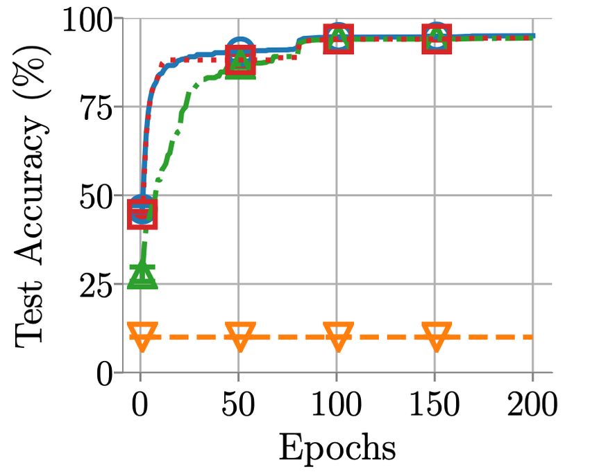
PipeMare: Asynchronous Pipeline Parallel DNN Training

                                  F2                       F0             F1           F2                F0           F1        F2

                                                           B0          B1              B2                B0           B1        B2

            (a) Throughput-Poor                                 (b) Memory-Hungry                                (c) PipeMare

Figure 1. Different extremes of pipelining modes. Orange squares represent model weight memory, blue circles represent active pipeline
compute, green clouds represent pipeline bubbles, and dashed gray lines separate pipeline stages. PipeMare fully utilizes compute while
minimizing weight memory footprint.

                                                Per Stage (i)                                          Overall
                                           τfwd,i             τbkwd,i                       Util                    Mem
                                       l           m
                                         2(P −i)+1                                                        PP
             PipeDream                       N                 τfwd,i                       1.0              |(w)i | · τfwd,i
                                                                                                              i=0
                                                                                           N
                                                                                                             PP
             GPipe                     l      0        m              0                 N +P −1           W = i=0 |(w)i |
                                           2(P −i)+1                                                         PP
             PipeMare                          N                      0                     1.0           W = i=0 |(w)i |

Table 1. Characterization of pipeline parallel training methods. τfwd and τbkwd are the pipeline delays for model weights in the forwards
and backwards pass. W is one copy of the weights. P is the number of pipeline stages. N is the number of microbatches in a minibatch.
i indexes the pipeline stage. |(w)i | denotes the number of weights in the ith pipeline stage.

the hardware) and/or memory (by storing additional weight                        • In Section 4, due to the lack of publicly available
copies for microbatching) (Harlap et al., 2018; Huang et al.,                      dataflow accelerators, we simulate PipeMare’s asyn-
2018). Importantly, these costs increase with the pipeline                         chronous training algorithm to evaluate it’s effective-
depth (as illustrated in Figure 1) even though the intention                       ness on both ResNet50 and Transformer models. We
of increasing the pipeline depth is to improve throughput.                         show that PipeMare can achieve competitive model
While these results are sufficient in the low-pipeline depth                       accuracy with better pipeline utilization than previous
setting, this poses a massive challenge for the type of high-                      approaches (GPipe and PipeDream).
depth, fine-grained pipeline parallelism of interest to new
hardware accelerators.                                                         1.1   Related Work
Motivated by enabling fine-grained pipeline parallelism on
                                                                               PipeDream.         PipeDream (Harlap et al., 2018) is
new hardware accelerators, in this paper we study how to
                                                                               a pipeline parallel distributed training technique used
remove hardware overheads during pipeline parallel train-
                                                                               to reduce high communication-to-computation ratios.
ing by revisiting the fundamental question: is preserving
                                                                               PipeDream showed up to 5x speedups in time-to-given-
synchronous execution necessary during neural network
                                                                               accuracy metrics when compared to existing data paral-
training? Our contributions and outline are as follows.
                                                                               lel training techniques. Unlike PipeMare, PipeDream is
                                                                               one type of memory hungry pipelining approach; their core
   • In Section 2, we introduce a model for asynchronous                       technique is called weight stashing which maintains an ad-
     pipeline-parallel training, that, by eschewing syn-                       ditional copy of the weights for each minibatch flowing
     chronous execution, maximizes hardware efficiency                         through the pipeline. This ensures synchronous computa-
     by avoiding both pipeline bubbles and substantial                         tion with a fixed pipeline delay update.
     memory increases.
                                                                               GPipe.        GPipe (Huang et al., 2018) is a pipeline par-
   • Using this model, in Section 3 we propose PipeMare,                       allel distributed training technique originally deployed on
     a system of two techniques to improve the statistical                     TPUs (Jouppi et al., 2017). Unlike PipeMare, GPipe is one
     efficiency of asynchronous pipeline training.                             type of throughput poor pipelining approach; the core tech-
PipeMare: Asynchronous Pipeline Parallel DNN Training
GPipe PipeDream PipeMare
1.0 1500 96.0
Weight + Opt. (MB)
Best Accuracy
Pipeline Util
95.5
1000
0.5 95.0
500
94.5
0.0 0 94.0
20 80 140 200 20 80 140 200 20 80 140 200
Pipeline Stages Pipeline Stages Pipeline Stages
Figure 2. The impact of the number of pipeline stages on pipeline utilization, weight memory, and final model quality across different
pipeline parallel training methods on a ResNet50 for image classification with the CIFAR10 dataset. Unlike PipeMare, GPipe and
PipeDream suffer hardware costs (either throughput or the sum of weight and optimizer memory) proportional to the number of pipeline
stages. Still, PipeMare achieves a final model quality competitive with the best technique.
nique used in GPipe is microbatching to hide the latency are random and can vary from step to step and weight
from introducing bubbles into the pipeline. This preserves to weight, unlike the fixed pipeline delay of the pipeline-
synchronous execution. This approach requires extra acti- parallel setting. In Appendix E we show PipeMare can
vation memory to preserve synchronous execution across also improve final model quality in this setting (Recht et al.,
batch boundaries; the authors use gradient checkpointing 2011a).
(Chen et al., 2016b) to alleviate this memory cost (see Ap-
pendix A.2 and appendix D for how PipeMare can do the 2 P RELIMINARIES
same). Using these techniques, they show that pipeline par-
allel can enable training larger models than ever on TPUs. Pipeline-parallel training of a DNN works by decompos-
In this paper, we focus on leveraging microbatching to re- ing the O operators of the neural network into P pipeline
duce asynchrony, but we also validate that, like GPipe, stages, each of which is assigned to a parallel worker (this
PipeMare can leverage gradient checkpointing to reduce worker can range from a fully distributed machine to a sec-
activation memory. tion of silicon on an accelerator). An operator here refers to
kernel level operators such as matrix multiplcation, ReLU,
Emerging Hardware Accelerators Recently there has or convolution. Each of these operators can be placed in
been a number of companies and academic work focused its own pipeline stage or many of them (like matrix multi-
on creating hardware accelerators designed specifically for plication, bias addition, and ReLU or convolution and nor-
deep learning training. A common characteristic in many malization) can be fused in the same stage (to save memory
of these deep learning accelerators is that they contain a or balance stage latencies). While processing a minibatch
large amount of SRAM on chip (Ward-Foxton; Feldman, of size B, each pipeline stage processes M samples at a
2019; Ward-Foxton, 2019a). This large amount of SRAM time, where M is called the microbatch size and M ≤ B.
enables these accelerators to consider dataflow execution of We use N to represent the number of microbatches in a
B
deep learning models, where the entire deep learning com- minibatch (or N = d M e) and let i represent a pipeline
putation graph can be mapped to a single accelerator at one stage. Operators can be associated with weights: we let
time. This paper is focused on providing an efficient train- W represent the total size of all these weights. The re-
ing mechanism for this emerging type of hardware accel- sulting microbatch gradients are accumulated into gradient
erators. Although this is our primary target our techniques buffers, and weights are updated only at minibatch bound-
can also be applied to model parallel training across mul- aries. Previous work studied the distributed case where
tiple accelerators (such as traditional GPU based architec- P
O: we call this coarse-grained pipeline parallelism.
tures or this new class of dataflow hardware accelerators). Here, we are interested in the case of fine-grained pipeline
parallelism, where P ≈ O. Using these definitions, we
Hogwild! Asynchronous training has been studied in compare PipeMare to the existing pipeline parallel training
several other contexts, the most well-known of which is techniques of PipeDream and GPipe in Figure 1 and Table 1
Hogwild! (Recht et al., 2011b). In Hogwild! settings, as (see Appendix A.1 for the derivation of each). The tradeoff
in pipeline-parallel settings, gradients are computed based between pipeline utilization, weight memory, statistical ac-
on delayed versions of weights. However, these delays curacy and pipeline stages are summarized in Figure 2 andPipeMare: Asynchronous Pipeline Parallel DNN Training
GPipe PipeDream PipeMare PipeMareW
1.0
Weight + Opt. (GB)
2.0 34
0.8
Pipeline Util
Best BLEU
1.5
0.6 5
1.0
0.4
2.5
0.5
0.2
0
0.0
40 80 120 160 200 40 80 120 160 200 40 80 120 160 200
Pipeline Stages Pipeline Stages Pipeline Stages
Figure 3. The impact of the number of pipeline stages on pipeline utilization, weight and optimizer memory, and final model quality
across different pipeline parallel training methods on a 12-layer Transformer model performing machine translation on the IWSLT14
dataset. Similar to image classification task, GPipe and PipeDream suffer hardware costs proportional to the number of pipeline stages.
Without these costs, PipeMare can achieve a final model quality close to the best technique and with a few warm-up epochs, PipeMareW
(with warmup epochs, see Section 4) can further close the gap. The target BLEU score chosen to evaluate the amortized pipeline
utilization of PipeMareW is 33.9.
Figure 3 and discussed in following sections. of the weights for that stage after t gradient updates have
been written to it (this means wt as a whole is not neces-
Pipeline Utilization/Throughput. Pipeline utilization
sarily the value of the weights in memory at any time t),
(Util) is the percentage of pipeline stages that are not idle
and the delayed weight values are defined for each pipeline
(stalled) at any given time. In the best case, when the num-
stage i ∈ {1, . . . , P } as
ber of active pipeline stages (Pactive ) equals the total num-
ber of pipeline stages (P ), we get 100% pipeline utilization
(ufwd,t )i = wt−τfwd,i and (ubkwd,t )i = wt−τbkwd,i
or Util = d Pactive
P = 1.0e. Note that throughput is linearly i i
proportional to Util. where (·)i denotes selecting the weights for the ith stage.
Delay. The statistical effect of using pipeline-parallel Here, we are letting ∇ft (ufwd,t , ubkwd,t ) denote the value
training is characterized by the pipeline delay: the num- of the gradient that would be computed by the backprop-
ber of optimizer steps that pass between when the weights agation algorithm using the weights ufwd,t in the forward
are read to compute a gradient and when that gradient is pass and weights ubkwd,t in the backward pass. That is,
used to update the weights. In a standard backpropagation ∇ft is a function of two weight vectors, rather than one
algorithm, each weight is read twice—once in the forward (as is usual for SGD), because the pipeline-parallel model
pass, and again in the backward pass—so there are two de- may use different values for the weights in the forward
lay values, τfwd and τbkwd , which can vary by stage. In- and backward pass. Synchronous execution corresponds
tuitively, τfwd corresponds to the delay between a weight’s to the case of ufwd,t = ubkwd,t , which requires setting
forward pass and its update. The earlier a pipeline stage, τfwd = τbkwd . For the rest of this paper, we will use
the larger τfwd value, i.e., τfwd,i ∝ (P − i) for the ith stage. ∇ft with two arguments to denote this backpropagation-
Similarly, τbkwd is the delay between a weight’s backward with-different-weights gradient, and use ∇ft with one ar-
pass and its update. We can write this out formally as gument to denote the ordinary mathematical gradient (un-
der this notation, ∇ft (w, w) = ∇ft (w) by definition).
wt+1 = wt − α∇ft (ufwd,t , ubkwd,t ) Techniques to date have not shown how to train well when
τfwd − τbkwd 6= 0.
where wt are the weight values after t gradient steps, ∇ft is
the gradient function for the t-th minibatch, and ufwd,t and 3 P IPE M ARE
ubkwd,t are the (delayed) values of the weights that are used
in the forward and backward passes, respectively, for com- We design a strategy called PipeMare for asyn-
puting ∇ft . The weights wt can be broken up into weight chronous pipeline-parallel training of deep neural net-
vectors for each stage: (wt )1 for stage 1, (wt )2 for stage 2, works. PipeMare combines two techniques, which we in-
et cetera, such that wt = [(wt )1 , (wt )2 , . . . , (wt )P ]. Con- troduce in this section, motivated by theory. For each tech-
cretely, the weight value (wt )i for stage i denotes the value nique, we start by modeling a problem we want to addressPipeMare: Asynchronous Pipeline Parallel DNN Training
4
Sync. τfwd,i = τbkwd,i , 107 stages τ =0 1024 ∞
theoretical bound
τfwd,i 6= τbkwd,i , 107 stages τfwd,i = τbkwd,i , 1712 stages τ =5
training loss
3 256
Delay (τ )
τ = 10 70
95 64
Loss
Test Accuracy (%)
Parameter Norm
1000 2 16 60
90 4
1 50
1
500 0 40
85 2−12 2−10 2−8 2−6 2−4 2−2
0 100 200
Iteration Step size (α)
80
0 10 20 30 40 50 60 0 50 100 150 200 (a) (b)
Iterations (102 ) Epochs
Figure 5. (a) Increasing τ can cause the quadratic model to di-
Figure 4. Analysis on the divergence for asynchronous pipeline- verge even when α remains fixed. (b) Evaluation of pipeline-
parallel training on ResNet50 training on the Cifar-10 dataset: parallel SGD for linear regression on the cpusmall dataset run-
the divergence is caused by the forward delay τfwd,i ; it is fur- ning for T = 106 iterations. The heatmap reports losses as a func-
ther exacerbated by forward-backward delay discrepancy when tion of the step size α and the delay τ ; red denotes divergence to
τfwd,i 6= τbkwd,i . Specifically in the left plot, we observe that ∞. The black curve shows the upper bound from Lemma 1 using
using 1712 stages without forward-backward delay discrepancy, the largest curvature of the objective in place of λ.
asynchronous training diverges at the beginning. We also ob-
serve that with 107 stages, asynchronous training diverges with
forward-backward delay discrepancy, while it does not diverge sults. In the next section we will show that this same phe-
without forward-backward delay discrepancy; this indicates that nomena we observe in deep learning matches our results on
delay discrepancy can exacerbate the divergence behavior. These the quadratic model. We use this quadratic model to under-
observations motivates us to explore the technique to stabilize stand the phenomena further and apply our findings back to
asynchronous pipeline-parallel training. deep learning examples. In more detail, for ResNet50 with
standard hyperparameters, Figure 4 shows that this phe-
by studying fixed-delay asynchronous gradient descent on nomenon is caused by the delay: the red series shows that,
a one-dimensional convex quadratic objective. Even this even when τfwd,i = τbkwd,i in simulation, substantially large
very simple “toy” model has non-trivial behavior, and (as fixed delay can cause the system to diverge. Figure 4 also
we will see) it exhibits many phenomena of interest seen illustrates that this divergence is exacerbated by forward-
in more complicated settings, and it motivates techniques backward delay discrepancy: the orange series shows that
to address them that work even for much more complicated even when the learning rate and delay τfwd,i are kept the
objectives (such as for DNNs). Consider a one-dimensional same, adding delay discrepancy can cause the algorithm to
quadratic objective f (w) = λw2 /2 for some fixed curva- diverge.
ture λ > 0. Suppose that we run fixed-delay asynchronous
SGD on this model, using gradient samples of the form 3.1 Learning rate rescheduling (T1)
We theoretically derive our first technique—rescheduling
∇ft (ufwd,t , ubkwd,t ) = λufwd,t − ηt = λwt−τ − ηt
the step size to be inversely proportional to the delay—and
where ηt is some gradient estimation noise, which we as- evaluate its tradeoffs on some DNN tasks.
sume is bounded and depends on t. This implicitly assumes The problem. We might hope that existing hyperparame-
that the delays for all the weights are the same and equal to ters used for sequential SGD would “just work” for train-
some fixed parameter τ = τfwd , with no delay discrepancy ing in the asynchronous pipeline parallel setting. Unfortu-
(we will consider delay discrepancy later in Section 3.2). nately, when we try running naively with a standard step
Running SGD in this setting has the update step size scheme, asynchronous pipeline parallel SGD can sig-
nificantly underperform the synchronous baseline. This
wt+1 = wt − α∇ft (· · · ) = wt − αλwt−τ + αηt . (1) happens because a large value of τ can cause SGD to di-
verge even when using a step size α for which the base-
line synchronous algorithm converges. This is shown in
Motivating example in deep learning Figure 4 illus-
Figure 5(a), which simulates the quadratic model (5) with
trates that, just as we saw for the quadratic model, pipeline-
λ = 1, α = 0.2, and ηt ∼ N (0, 1), for various values of
parallel SGD can not be run naively with the same hyper-
τ . Notice that for τ = 10, the trajectory diverges quickly.
parameters as would be used in the baseline model, since
In Section 3, we show that the same phenomenon can be
this would significantly negatively impact loss. Figure 4
observed for a ResNet50 network.
shows why: pipeline-parallel SGD is diverging to infin-
ity, completely failing to learn, even for a step size scheme The theory. The first question we want to ask is: when
for which the sequential model achieves state-of-the-art re- will asynchronous pipeline-parallel SGD be stable on thePipeMare: Asynchronous Pipeline Parallel DNN Training
quadratic model? That is, for what values of the step size 4 1.3
Largest eigenvalue
∆=0 Discrepancy,
α will it be guaranteed that wt remains bounded, no matter 3 ∆=3 1.2
no correction
No discrepancy
∆=5
what (bounded) noise signal ηt we get from the gradient (∆ = 0)
Loss
Discrepancy
2 1.1 correction
estimator? To answer this question, notice that (1) is a lin- (D = 0.1)
ear system, which can be written in terms of a companion 1 1.0
matrix that stores all the state of the system as 0 0.9
0 100 200 0.01 0.1 1.0
wt+1 " # wt " αη #
1 0 ··· 0 −αλ t Iteration Step size (α)
wt 1 0 ··· 0 0 wt−1 0
.. = .. .. . . .. .. . + .. .
. (a) (b)
. . . . . . . .
wt−τ +1 0 0 ··· 1 0 wt−τ 0
Figure 6. (a) Increasing ∆, the gradient sensitivity to delay dis-
If we call this companion matrix C, and call the vectorized crepancy, can cause the quadratic model to diverge even when α
version of w with its history W , and τ remain fixed, using τfwd = 10, τbkwd = 6, and λ = 1. (b)
Effect of discrepancy correction on the quadratic model. Forward-
Wt+1 = CWt + αηt e1 , (2) backward delay discrepancy (blue) increases the largest magni-
T tude eigenvalue of the companion matrix with ∆ = 5, and τ , λ
where e1 is the vector 1 0 · · · 0 . Linear systems same as in (a). Discrepancy correction with D = 0.1 (orange) re-
of this type have solutions of the form duces the largest magnitude eigenvalue; this eigenvalue is closer
Pt−1 to that attained without delay discrepancy (green).
wt = k=0 αηt−k−1 ω ρω (k) · ω k ,
P
where the sum here ranges over the eigenvalues ω of the
companion matrix, and each ρω is a polynomial of degree The technique. To avoid the divergence we just charac-
less than the algebraic multiplicity of the eigenvalue ω.1 terized, the natural choice here is to divide the step size at
Thus, the convergence of (2) is determined entirely by C’s each pipeline stage i by its delay τi . However, this is (1)
eigenvalues, and it will be stable when all these eigenvalues problematic because it leads to very small step sizes which
lie inside the unit disk in the complex plane. C’s eigenval- slow convergence, and (2) unnecessary because it divides
ues are the zeros of its characteristic polynomial the step size by τ even for later epochs where the base step
size has already become small, as is usually done in deep
p(ω) = ω τ +1 − ω τ + αλ. (3) learning (He et al., 2016; Vaswani et al., 2017). This moti-
vates us to develop a step size scheme that (1) behaves like
So we want to find out for which values of α the roots of p the O(τ −1 ) scheme for early epochs, and (2) degrades back
must all lie inside the unit disk. to the baseline learning rate scheme for later epochs.
Lemma 1. The roots of the polynomial p of (3) all lie inside
T1: Suppose that we are training a DNN. In SGD step k,
the unit disk if the step size α is
assign the following step size to pipeline stage i.
2 π 1
0 ≤ α ≤ · sin =O .
λ 4τ + 2 λτ αk,base k
αk,i = where pk = 1 − min ,1 . (4)
τipk K
This lemma gives us theoretical insight that backs up our
empirical observations: when the delay is larger, the step where K is a hyperparameter representing a number of
size must be set smaller to prevent instability and diver- steps during which to adjust the learning rate, and αk,base
gence. It also quantifies how much smaller, predicting that denotes the normal synchronous learning rate. We sug-
α should be set as O(τ −1 ). In Figure 5(b) we validate that gest K to be 41 the length of the first phase of a fixed-step
our theory not only applies to 1D optimization problems, LR schedule (we use this for the ResNet model) or five times
but also can accurately describe what happens when we run the linear warmup steps of a schedule with a linear warmup
pipeline-parallel SGD on a simple 12-dimensional linear phase (we use this for the Transformer model).
regression problem using the cpusmall dataset (Chang &
Lin, 2011); the algorithm diverges at precisely an α ∝ τ −1 3.2 Discrepancy correction (T2)
slope, exactly what Lemma 1 predicts. In Appendix B.2 we
extend this to momentum SGD showing that the O(τ −1 ) In Section 3.1, we analyzed a setting in which there was
threshold is general, which motivates our use of Technique no delay discrepancy (τfwd = τbkwd ). In this subsection,
1 with algorithms other than SGD such as Adam. we try to understand the effect of delay discrepancy, again
using our quadratic model. We then develop and evaluate a
1
To see why, consider the Jordan normal form of C, which technique for “correcting” this discrepancy.
will for each eigenvalue have a corresponding Jordan block of
dimension equal to its algebraic multiplicity. The problem. To model delay discrepancy, we now as-PipeMare: Asynchronous Pipeline Parallel DNN Training
sume gradient samples of the form of divergence. If we could just compute ∇ft (ufwd,t , ufwd,t )
directly, then this mismatch would not be a problem. Un-
∇ft (ufwd,t , ubkwd,t ) = (λ + ∆) · wt−τfwd − ∆ · wt−τbkwd − ηt fortunately, in our asynchronous pipeline parallel setting
we cannot compute this, as we no longer have ufwd,t in
where τfwd > τbkwd are two different delays, and ∆ is a memory by the time the backward pass comes around . To
constant that measures the sensitivity of the gradients to keep ufwd,t stored in memory is possible, but undesirable as
discrepancy. We can think of this as the natural first-order it would greatly increase memory usage (as in PipeDream).
(linear) approximation of ∇ft in the neighborhood of a Instead, we decrease the gap between ufwd,t and ubkwd,t
stationary point—it models any affine function of ufwd,t by approximating ufwd,t without storing the full history of
and ubkwd,t that is consistent with the curvature λ when model weight values after ufwd,t , using a bit of extra mem-
ufwd,t = ubkwd,t . If ∆ = 0, we recover a model of our orig- ory to hold an approximation of the velocity of the weights.
inal zero-discrepancy setting, whereas for large-magnitude
values of ∆, even a small delay discrepancy could be am- T2: Instead of the assignment of ubkwd from Section 3.1, set
plified to have a large effect on the gradient samples.
(ubkwd,t )i = wt−τbkwd,i i − (τfwd,i − τbkwd,i ) δt,i ,
Delay discrepancy is problematic because it can amplify
the divergence effect observed in Section 3.1. To illustrate, where δt,i is a accumulator that estimates the amount that
Figure 6(a) shows on the quadratic model (with τfwd = 10, wi is changing over time. It is kept up to date by the up-
τbkwd = 6, λ = 1, and ηt ∼ N (0, 1)) that a nonzero value date step δt+1,i = γi · δt,i + (1 − γi ) · (wt+1,i − wt,i ),
of ∆ can cause divergence even for a value of α and τ where γi is a decay rate parameter, assigned per-stage to
where with ∆ = 0 (i.e. running PipeDream-style with no γi = D1/(τfwd,i −τbkwd,i ) , where D is a tunable global hyper-
discrepancy) the trajectory would converge. In Section 3, parameter.
we illustrate that, just as was the case for the divergence Essentially, this technique adjusts the value of the weights
phenomenon of Section 3.1, on ResNet50 asynchronous used in the backward pass by extrapolating what the
SGD with a large enough ∆ will diverge even for values of weights were during the forward pass based on the re-
α and τ for which PipeDream-style SGD converged. We cent average trajectory of the weights. Applying T2 on
seek to understand this phenomenon theoretically and to the quadratic model also results in an update step that
develop a technique to limit its effect. can be modeled with a companion matrix; we analyzed
The theory. With our new discrepancy-dependent samples, this system—just as before—by considering that compan-
pipeline parallel SGD has the update step ion matrix’s eigenvalues. Doing this, we observed that T2
seems to increase the allowable range of α for which the
wt+1 = wt − α(λ + ∆)wt−τfwd + α∆wt−τbkwd + αηt . (5) quadratic model is stable. This is illustrated in Figure 6(b).
As before, we can analyze this for stability by finding the
value of α for which the roots of its characteristic polyno-
4 E XPERIMENTS
mial lie inside the unit disk. We simulate PipeMare on two standard image recognition
Lemma 2. For any ∆ > 0, there exists an α > 0 with tasks and neural machine translation tasks to evaluate its
effectiveness. Our evaluation supports the following two
2 2 π main claims:
α ≤ min , · sin
∆ · (τfwd − τbkwd ) λ 4τfwd + 2
• PipeMare can enable more efficient end-to-end train-
such that at least one of the roots of the characteristic poly- ing on new dataflow accelerators. We show that across
nomial of (5) is outside the interior of the unit disk (that is, two image recognition and two neural machine translation
the disrepancy-dependent model updates will be unstable). tasks, PipeMare can attain up to 14.3× higher pipeline uti-
lization over the synchronous GPipe and uses up to 2.7×
This lemma shows two important things: first, that the max- less weight and optimizer memory when compared to the
imal stable step size is still inversely proportional to the de- synchronous PipeDream.
lay, even with delay discrepancy; second, that for large val- • PipeMare achieves final model qualities similar to
ues of ∆, in which the delay discrepancy has substasntial those attained by synchronous training. We show that
effect on the gradient, the largest stable α becomes smaller PipeMare at most has a top-1 test accuracy difference of
(although still inversely proportional to τ ). This models 0.1% compared to synchronous baselines on image recog-
the behavior illustrated in Figure 6(a) where adding delay nition tasks and matches synchronous baselines on transla-
discrepancy exacerbates the divergence phenomenon. tion tasks.
The technique. As shown, delay discrepancy between the Warmup Epochs (W). In some cases, the statistical
forward and backward passes can exacerbate the problem (hardware)-efficiency tradeoff PipeMare presents is tooPipeMare: Asynchronous Pipeline Parallel DNN Training
Table 2. Comparison of statistical efficiency (test accuracy or BLEU score), (amortized) pipeline utilization, and weight+optimizer mem-
ory of PipeMare(W) and baselines. Here we use top-1 accuracy or BLEU score as the metrics for CIFAR10/ImageNet and IWSLT/WMT
respectively. Target accuracies (BLEU scores) for each task are 94.0(CIFAR10), 75.5(ImageNet), 34.1(IWSLT) and 27.4(WMT).
Dataset Method Acc. Pipe. Util. Memory
PipeDream 94.8 100% 2.70X
CIFAR10 GPipe 95.0 7% 1X (270MB)
PipeMare 95.0 100% 1.33X
PipeDream 74.7 100% 1.61X
GPipe 76.0 13% 1X (293MB)
ImageNet
PipeMare 75.5 100% 1.33X
PipeMareW 75.9 33% 1.33X
Dataset Method BLEU Pipe. Util. Memory
PipeDream 0.0 100% 2.06X
GPipe 34.5 17% 1X (0.65GB)
IWSLT14
PipeMare 34.1 100% 1.25X
PipeMareW 34.5 42% 1.25X
PipeDream 0.0 100% 2.39X
GPipe 27.5 56% 1X (1.01GB)
WMT17
PipeMare 27.0 100% 1.25X
PipeMareW 27.8 96% 1.25X
coarse-grained. Here, we use the standard technique of run- from runs with three different random seeds.
ning a number of warmup epochs of the baseline method
before switching to PipeMare to trade off hardware effi-
ciency for statistical efficiency. Concretely, we initialize Implementation Details All experiments are run using a
with Ew epochs of synchronous (GPipe-style) pipeline- simulator we built in PyTorch and on AWS p3.2xlarge in-
parallel training using the standard learning rate. We stances (Nvidia V100 GPUs). To design our simulator we
call this modified method PipeMareW. Since we intro- changed the optimizer module in PyTorch to simulate the
duce synchronous training in the beginning, the average exact delay one would see when computing updates while
pipeline utilization U tilP ipeM areW is amortized over the running with fine-grained pipeline parallelism. To do this
total time needed to reach a target accuracy (BLEU score), our custom optimizer implementation maintains a queue of
EP ipeM are +ESync
i.e., E 1 , where E denotes epochs. stale weight values2 that represents the delay one would get
P ipeM are+E ×
Sync U tilSync
in each pipeline stage. With our simulation we model the
statistical effects of this fine-grained pipeline parallelism,
4.1 Experimental Setting propose compute and memory friendly techniques to coun-
We overview the details of our experimental setup and pro- teract these effects, and experiment with our techniques on
vide the exact details in Appendix C. real deep neural networks. This enables our goal of provid-
ing theoretical and experimental evidence to help validate
Setup. Since the purpose of this paper is to determine if the design, efficacy, and potential of new dataflow acceler-
asynchronous pipeline parallel is feasible statistically (and, ators.
if successful, enable emerging hardware accelerator de-
signs to reap the hardware benefits), we built a custom op- Benchmarks. We benchmark a ResNet50 model (He
timizer in PyTorch that simulates (running on Nvidia V100 et al., 2016) for image classification and the 12-layer Trans-
GPUs) the exact asynchronous updates (via a queue of stale former model (Vaswani et al., 2017) for neural machine
weights) of PipeMare. Using this, we report the pipeline translation (mlp, 2019). We use the standard CIFAR10
utilization, weight and optimizer memory, and accuracy (or and ImageNet datasets for image classification, and pop-
BLEU score) on each benchmark. The pipeline utilization ular IWSLT14 German-to-English and WMT17 English-
and memory we report are calculated using the formulas we 2
We only maintain such a queue for simulation purposes, no
present in Table 1. We report the averaged model accuracy extra copy of stale weights is needed in real dataflow accelerators.PipeMare: Asynchronous Pipeline Parallel DNN Training
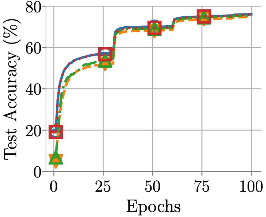
to-German dataset for neural machine translation. We Sync. PipeMare T1 PipeMare T1 + T2 PipeMare T1 + T2 + W
use standard, publicly available hyperparameters (see Ap- 100
35
Test Accuracy (%)
pendix C.1) for each of these two popular models. For im-
75
BLEU Score
age classification, we use test set accuracy as the model 30
50
accuracy metric while in translation tasks we use test 25
BLEU score. We compare PipeMare to two synchronous 25
20
(baseline) pipeline parallel training methods: GPipe and 0
0 50 100 150 200 0 12 24 36 48 60
PipeDream. We report in detail on the two non-standard Epochs Epochs
hyperparameters we had to select next (microbatch size and
number of pipeline stages). For all other hyperparameters
Figure 7. The impact of incrementally combining PipeMare tech-
we use standard, publicly available hyperparameters (see niques (T1, T2, and W) with ResNet50 on Cifar10 (left) and
Appendix C.1) for each of these two popular models. Transformer on IWSLT14 (right) with 107 and 93 pipeline stages
Microbatch Size. For microbatch size (M ) we always respectively. Runs are stable across seeds indicated via the (neg-
ligible) error bars in each plot.
select a value that is as small as possible. This has two
main benefits: (1) it saves activation memory and (2) it
results in less gradient delay τf wd given a fixed number
of pipeline stages (more microbatches per minibatch). We
choose M = 8(16) for ResNet50 on CIFAR10 (ImageNet)
as smaller M , in both cases, cause problems in batch nor-
malization (Yuxin Wu, 2018) operators. For Transformer
on IWSLT14 we choose the number of tokens (245) in the
longest sentence as the maximum tokens per microbatch.
On WMT17, we used a maximum tokens per microbatch
of 1792 for both PipeDream and PipeMare, as this enabled
results to be simulated within a reasonable timeframe. To
be fair, in GPipe pipeline utilization calculation, we maxi- Figure 8. The impact of incrementally combining PipeMare tech-
mized their efficiency by using a maximum tokens of 251 niques (T1, T2, and W) with ResNet50 on Cifar10 (left) and
(the longest sentence in WMT17). Transformer on IWSLT14 (right) with 214 and 186 pipeline
stages respectively. This doubles the number of pipeline stages
Pipeline Stages. To partition the model, we traverse as compared to Figure 7. It explores the limits of our approach at
model weights according to their topological order in the an even finer granularity of pipeline parallelism.
graph, always treating weight and bias in the same opera-
tor as a fused weight. Next, we split these model weights
evenly over P pipeline stages to represent the fine grained accuracy gap with GPipe on ImageNet but achieves 2.5×
pipeline parallelism which is hard to train. Specifically, we higher pipeline utilization (using 30 warmup epochs).
use 107 stages for ResNet50 and 93 stages for Transformer
in Section 4.2. Neural machine translation tasks Because we use
PipeMareW on both the IWSLT14 (10 warmup epochs) and
4.2 End-to-End Comparison WMT17 (4 warmup epochs) experiments the amortized
pipeline utilization of PipeMare is less than 100%, though
We compare the asynchronous PipeMare training method it still achieves 2.5× and 1.7× higher pipeline utilization
to the synchronous GPipe and PipeDream methods on both than GPipe. We observe that PipeDream fails to train
image classification and machine translation tasks. In Ta- Transformer even though it uses >2× more weight and
ble 2 we show that on both of these tasks PipeMare ob- optimizer memory than PipeMare. Therefore, PipeMare
tains higher pipeline utilization, uses less weight and opti- improves the pipeline utilization and memory usage when
mizer memory, and achieves comparable final model qual- compared to previous pipeline parallelism techniques, with
ities when compared to the synchronous baselines. no loss in statistical performance.
Image classification tasks On the CIFAR10 dataset,
PipeMare can achieve 14.3× higher pipeline utilization 4.3 Ablation study
than GPipe while maintaining same test accuracy. Note that To understand the contribution of each technique to the
on CIFAR10, PipeMare attains 100% pipeline utilization as performance of PipeMare, we perform ablation studies on
it does not need any warmup epochs. Though PipeDream PipeMare with respect to memory, pipeline utilization, and
attains the same utilization as PipeMare, it requires 2.7× model quality. We show that each technique is necessary
more weight and optimizer memory. PipeMareW has 0.1% for PipeMare to outperform synchronous techniques and isPipeMare: Asynchronous Pipeline Parallel DNN Training
Table 3. Ablation study of PipeMare. We show the impact of the learning rate rescheduling (T1), discrepancy correction (T2), and
warmup epochs (W) on metrics of interest. Note that warmup epochs were not necessary on the CIFAR10 dataset to recover the
performance of GPipe.
Dataset Method Acc. Pipe. Util. Memory
T1 Only 95.0 100% 1X (270MB)
CIFAR10 T2 Only 94.5 100% 1.33X
T1+T2 95.0 100% 1.33X
Dataset Method BLEU Pipe. Util. Memory
T1 Only 34.1 100% 1X (0.65GB)
T2 Only 0.0 100% 1.25X
IWSLT14
T1 + T2 Only 34.1 100% 1.25X
T1 + T2 + W 34.5 42% 1.25X
summarized in Figures 7 and 8 and table 3. on IWSLT14, as is seen in Figure 7 and Figure 8. This of
course comes at the cost of using more weight memory, but
Learning rate rescheduling (T1). Asynchronous pipeline
it is minimal (33% more for SGD with momentum and 25%
parallel training with only T1 fully utilizes the compute
more for ADAM) given the improvements in training speed
power by avoiding bubbles and additional weight stash-
and accuracy. To further validate the efficacy of T2, in Ap-
ing. Therefore it achieves optimal hardware efficiency.
pendix C.2.2, we show that on a ResNet152 model with 150
T1 alone can achieve a test accuracy (BLEU score) of
stages T2 is necessary to prevent divergence and match the
95.0% (34.1), competitive to the baseline of synchronous
accuracy attained by synchronous training. T2 alone either
methods (95.0% accuracy and 34.5 BLEU score), and im-
fails to converge or archives a suboptimal accuracy. How-
prove pipeline utilization by up to 14.3× over GPipe. For
ever when combined with T1, as shown in Figure 8 again,
ResNet50 on CIFAR10, the test accuracy of asynchronous
can enable or accelerate convergence.
training with T1 matches that of synchronous training
while asynchronous training without it diverges; for the Warmup Epochs (PipeMareW). T1 and T2 still leave
Transformer model, T1 takes about twice as many epochs a noticeable BLEU score gap (0.4) for Transformer on
of synchronous training to reach BLEU score 34.1 while IWSLT14 (Table 3). To close this gap PipeMareW adds
asynchronous training without T1 achieves a test BLEU 10 synchronous warmup epochs. The best BLEU score
score ≤ 1. This indicates that T1 does a lot of the heavy is boosted from 34.1 to 34.5. This comes at the cost
lifting in boosting hardware efficiency while maintaining of decreasing the overall pipeline utilization of PipeMare
statistical efficiency as shown in Table 3 and Figure 7. from 100% to 42%, which is still significantly higher than
However, as shown in Figure 8, T1 alone cannot prevent GPipe.
diverge (in ResNet50) or can only achieve a much worse
BLEU score (in Transformer). Therefore the efficacy of T1 5 C ONCLUSION
weakens as the number of pipeline stages increases which
can be solved when T2 (discussed next) is combined with In this paper, we presented PipeMare, a system for
T1. asynchronous pipeline-parallel training of DNN models.
PipeMare uses a bubble-free pipeline parallel hardware
Discrepancy Correction (T2). T2 mitigates the discrep-
model along with two theoretically motivated techniques
ancy from delay and helps accelerate convergence. Our
(learning rate rescheduling and discrepancy correction)
experiment results indicate that in addition to T1, T2 is
which help improve statistical efficiency. Experimen-
also an important technique to achieve state of the art re-
tally, we showed PipeMare has better hardware efficiency
sults on certain models. As shown in Table 3, T2 alone
(pipeline utilization and memory) than competing algo-
achieves an accuracy of 94.5% on ResNet50 while a jar-
rithms. We hope that this will make PipeMare a promis-
ring 0.0 BLEU score on Transformer model. The poor per-
ing candidate algorithm for the new generation of hardware
formance of Transformer is fixed by combining T2 with
chips designed for training DNNs.
T1, though the final test BLEU score (34.1) is the same
as in T1 only setting. T2 with T1 shines on the conver-
gence speed of both models, especially Transformer modelPipeMare: Asynchronous Pipeline Parallel DNN Training
ACKNOWLEDGEMENTS Kurth, T., Zhang, J., Satish, N., Racah, E., Mitliagkas, I.,
Patwary, M. M. A., Malas, T., Sundaram, N., Bhimji,
We are grateful to Sumti Jairath and Zhuo Chen for their W., Smorkalov, M., et al. Deep learning at 15pf: su-
insightful discussions. We thank David Luts and the anony- pervised and semi-supervised classification for scientific
mous reviewers for their valuable feedbacks. data. In Proceedings of the International Conference for
High Performance Computing, Networking, Storage and
R EFERENCES Analysis, pp. 7. ACM, 2017.
Fair and useful benchmarks for measuring training and in- Mitliagkas, I., Zhang, C., Hadjis, S., and Ré, C. Asyn-
ference performance of ml hardware, software, and ser- chrony begets momentum, with an application to deep
vices. 2019. URL https://mlperf.org/. learning. In 2016 54th Annual Allerton Conference on
Communication, Control, and Computing (Allerton), pp.
Chang, C.-C. and Lin, C.-J. LIBSVM: A library for sup-
997–1004. IEEE, 2016.
port vector machines. ACM Transactions on Intelli-
gent Systems and Technology, 2:27:1–27:27, 2011. Soft- Prabhakar, R., Zhang, Y., Koeplinger, D., Feldman, M.,
ware available at http://www.csie.ntu.edu. Zhao, T., Hadjis, S., Pedram, A., Kozyrakis, C., and
tw/˜cjlin/libsvm. Olukotun, K. Plasticine: A reconfigurable accelerator
for parallel patterns. IEEE Micro, 38(3):20–31, 2018.
Chen, T., Xu, B., Zhang, C., and Guestrin, C. Training
doi: 10.1109/MM.2018.032271058. URL https://
deep nets with sublinear memory cost. arXiv preprint
doi.org/10.1109/MM.2018.032271058.
arXiv:1604.06174, 2016a.
Recht, B., Re, C., Wright, S., and Niu, F. Hogwild: A
Chen, T., Xu, B., Zhang, C., and Guestrin, C. Train-
lock-free approach to parallelizing stochastic gradient
ing deep nets with sublinear memory cost. CoRR,
descent. In Advances in neural information processing
abs/1604.06174, 2016b. URL http://arxiv.org/
systems, pp. 693–701, 2011a.
abs/1604.06174.
Recht, B., Ré, C., Wright, S. J., and Niu, F. Hogwild:
De Sa, C. M., Zhang, C., Olukotun, K., and Ré, C. Taming
A lock-free approach to parallelizing stochastic gra-
the wild: A unified analysis of hogwild-style algorithms.
dient descent. In Advances in Neural Information
In Advances in neural information processing systems,
Processing Systems 24: 25th Annual Conference
pp. 2674–2682, 2015.
on Neural Information Processing Systems 2011.
Feldman, A. Cerebras wafer scale engine: An introduction. Proceedings of a meeting held 12-14 December
2019. URL https://www.cerebras.net/wp- 2011, Granada, Spain., pp. 693–701, 2011b. URL
content/uploads/2019/08/Cerebras- http://papers.nips.cc/paper/4390-
Wafer-Scale-Engine-Whitepaper.pdf. hogwild-a-lock-free-approach-to-
parallelizing-stochastic-gradient-
Harlap, A., Narayanan, D., Phanishayee, A., Seshadri, V., descent.
Devanur, N., Ganger, G., and Gibbons, P. PipeDream:
Fast and efficient pipeline parallel DNN training. arXiv Sutskever, I., Martens, J., Dahl, G., and Hinton, G. On
preprint arXiv:1806.03377, 2018. the importance of initialization and momentum in deep
learning. In International conference on machine learn-
He, K., Zhang, X., Ren, S., and Sun, J. Deep residual learn- ing, pp. 1139–1147, 2013.
ing for image recognition. In Proceedings of the IEEE
conference on computer vision and pattern recognition, Vaswani, A., Shazeer, N., Parmar, N., Uszkoreit, J., Jones,
pp. 770–778, 2016. L., Gomez, A. N., Kaiser, Ł., and Polosukhin, I. Atten-
tion is all you need. In Advances in neural information
Huang, Y., Cheng, Y., Chen, D., Lee, H., Ngiam, J., Le, processing systems, pp. 5998–6008, 2017.
Q. V., and Chen, Z. Gpipe: Efficient training of gi-
ant neural networks using pipeline parallelism. arXiv Ward-Foxton, S. Groq tensor streaming proces-
preprint arXiv:1811.06965, 2018. sor architecture is radically different. URL
{https://groq.com/groq-tensor-
Jouppi, N. P., Young, C., Patil, N., Patterson, D., Agrawal, streaming-processor-architecture-
G., Bajwa, R., Bates, S., Bhatia, S., Boden, N., Borchers, is-radically-different/}.
A., et al. In-datacenter performance analysis of a tensor
processing unit. In 2017 ACM/IEEE 44th Annual Inter- Ward-Foxton, S. Graphcore ceo touts ’most complex pro-
national Symposium on Computer Architecture (ISCA), cessor’ ever. EE Times, 2019a. URL {https://www.
pp. 1–12. IEEE, 2017. eetimes.com}.PipeMare: Asynchronous Pipeline Parallel DNN Training
Ward-Foxton, S. Habana debuts record-breaking ai train-
ing chip. EE Times, 2019b. URL {https://www.
eetimes.com}.
Wilson, A. C., Roelofs, R., Stern, M., Srebro, N., and
Recht, B. The marginal value of adaptive gradient meth-
ods in machine learning. In Advances in Neural Infor-
mation Processing Systems, pp. 4148–4158, 2017.
Yuxin Wu, K. H. Group normalization. arXiv preprint
arXiv:1803.08494, 2018.PipeMare: Asynchronous Pipeline Parallel DNN Training
A S UPPLEMENTARY MATERIAL GPipe. For GPipe, τfwd = τbkwd = 0, at the cost of lower
FOR S ECTION 2 pipeline utilization and additional activation memory. Each
pipeline has to be filled and drained at a minibatch bound-
To better explain the hardware efficiency of the pipeline ary to ensure weight synchronization between forward and
parallel training methods introduced in Section 2, we first backward pass, so the average bubble time is O( NP+P −1
−1 )
derive the memory footprint and utilization of the intro- (Huang et al., 2018). Consequently, the pipeline utilization
duced methods in more detail in Appendix A.1. In Ap- of GPipe is N +P N
−1 . GPipe leverages microbatching (in-
pendix A.2, we first discuss the activation memory which is creasing N > 1) to reduce the number of bubbles in its
the major component of memory consumption in pipeline- pipeline. GPipe does not store any additional weight mem-
parallel training. We then propose a new gradient check- ory but does store additional memory for activations. Us-
pointing method to trade moderate compute for signifi- ing the standard technique of gradient checkpointing (Chen
cantly lower activation memory footprint in Appendix A.3, et al., 2016b), both PipeMare and GPipe can reduce their
which is applicable to both the synchronous and asyn- activation memory footprint (see Appendix A.3 and ap-
chronous methods introduced in Appendix A.1. Finally, pendix D).
we discuss the throughput of the synchronous (GPipe) and
asynchronous (PipeDream and PipeMare) methods under PipeMare. In PipeMare we let the computation proceed
the same budget for activation memory and compute (mea- asynchronously: we just compute gradients with what-
sured in FLOPs), which is used to estimate the time-to- ever weights are in memory at the time we need to use
accuracy across the paper. Throughout the remainder of the them. This avoids any need to store extra copies of our
appendix we use normalized throughput instead of pipeline model weights (Mem = W ) or introduce bubbles into our
utilization as the two are linearly proportional to each other. pipeline (Util = 1.0), because as soon as a pipeline stage
has its gradients (accumulated within a full minibatch) the
To discuss with consistent notations across methods, we weights are updated. This means that the forward propa-
define M and N respectively as the activation size per mi- gation is done on different weights than those that are used
crobatch per neural net operator and the number of micro- for backpropagation, i.e., τfwd 6= τbkwd . Concretely, each
batches in each minibatch. We assume that we use models operator in our neural network has a fixed forward delay of
with L operators, which are trained using a pipeline with P τfwd = d 2(P −i)+1 e which is the same τfwd as PipeDream.
N
stages. For clarity and simplicity in exposing the memory On the other hand, since there is no delay between back-
footprint and throughput, we assume that the model opera- ward pass and weight updates, τbkwd = 0. Similar to GPipe,
tors are partitioned equally across stages and the activation minimizing the microbatch size M reduces the activation
memory usage of each operator is the same. memory usage while also keeping each pipeline stage fully
utilized. Unlike in GPipe, minimizing the microbatch size
A.1 Pipeline Parallel Training Methods in PipeMare has the additional benefit of helping to reduce
Using the setup from Section 2, we analyze the delays, the discrepancy between the forward and backward delays.
pipeline utilization, and memory usage of the two syn-
chronous baseline PP training methods (PipeDream and A.2 Activation Memory
GPipe), and we introduce the setup for our asynchronous PipeMare and PipeDream PipeMare and PipeDream
method (PipeMare). These results are summarized in Fig- has the same amount of activation memory requirement.
ure 1(d). This is because in both scenarios, pipeline does not have
PipeDream. PipeDream has forward delay τfwd,i = bubbles or stalls; the activations are cached and utilized
d 2(P −i)+1 e and uses weight stashing to cache the weights with the same pipeline behavior pattern. In particular, the
N
used in the forward pass until they are needed in the back- activation memory cached by stage i is proportional to
ward pass, which allows for full pipeline efficiency while the number of stages between forward and backward, i.e.,
maintaining synchronous execution τfwd = τbkwd . Note that O(2(P − i) + 1). Therefore, the total activation memory is
because τfwd = τbkwd PipeDream uses same weights for
both forward and backward passes, despite having a de-
AP M = O(M P L). (6)
layed update. Unfortunately, this comes at the cost of stor-
ing copies of the weights, which uses extra memory of size
GPipe Here we discuss on the activation memory con-
Mem = i=0 |(w)i |×τfwd,i = i=0 |(w)i |×d 2(P −i)+1
PP PP
N e.
sumption of GPipe (Huang et al., 2018). When the ac-
With fine-grained PP P can become large, making the over- tivations of every operator in neural nets are cached for
head Mem large, which presents a problem for large mod- backpropagation, by multiplying the activation memory per
els. Because PipeDream’s pipeline is fully utilized during minibatch per operator B = M N with the number of op-
training they have a pipeline utilization of Util = 1.0. erators L, we have the activation memory for GPipe asPipeMare: Asynchronous Pipeline Parallel DNN Training
A.3 Trade compute for memory via PipeMare
W/o recompute Recompute
W/ recompute In the fine-grain pipeline training setting, we have P ≈ L.
For simplicity in discussion, we assume P = L. In this
setting, eq. (6) becomes,
# of cached activations
30
AP M = O(M P 2 ). (8)
20
In other words, while throughput increases linearly with
number of stages P , activation memory can scale quadrat-
10 ically. In order to reduce the memory pressure, here we
propose a new way of utilizing recompute, to trade a small
amount of compute resources for huge activation memory
0 savings. Instead of recomputing the activations inside each
0 4 8 12 16 stage (Huang et al., 2018), we propose to recompute the ac-
Stage ID tivations across a segment of multiple stages, which we call
PipeMare Recompute, to allow effective activation memory
Figure 9. Activation memory footprint of PipeMare recompute in
reduction in the fine-grain pipeline setting.
each pipeline stage. In this plot, we demonstrate the # of activa- PipeMare Recompute utilizes a simple strategy. It recom-
tions at each stage using an example with 16 stages equally split putes the activation in advance so that the recomputed acti-
into 4 segments. The green bars in the plot stands for the memory vation of the last stage in a segment arrives right at the time
consumption of each stage in terms of the number of microbatch
when the corresponding backpropagation needs to process
activations copies in PipeMare with PipeMare recompute. The
orange bars stands for the additional memory required when re-
this activation. Unlike the single-stage recompute pro-
compute is not used. posed in GPipe (Huang et al., 2018), PipeMare Recompute
does not stall the backpropagation operations as it can be
overlapped with the forward and backward operations in
the same pipeline stage. To enable this overlap, we need
to consume approximately 25% of the total compute re-
AGP = O(M N L). (7) sources. Specifically, the pipeline needs to simultaneously
compute for the forward, backward and recompute opera-
tions, with the backward operations consuming 2× more
When re-materialization proposed by (Huang et al., 2018) compute than forward and recompute operations respec-
is considered, we only need to store the activations of a tively.
minibatch at every stage boundary, and recompute the acti-
vations for all the operators inside the stage. Therefore the For the simplicity of demonstrating the activation mem-
activation memory per stage is O(M N + M PL ), with the ory saving attained by PipeMare Recompute, we assume
total activation memory reduced to: P = L in the fine-grain pipeline setting and group the
stages into segments each with S stages. Let us assume
the i − th stage is the beginning stage of a specific seg-
ÃGP = O(M N P + M L) = O(M (N P + L)). ment, then the memory consumption for this segment is
O(2(P − i) + S 2 ). As visualized in Figure 9 for an exam-
ple with 16 stages and 4 segments, the first term 2(P − i)
When P
L, the saving on activation memory is signif- in the segment-wise activation memory is for caching acti-
icant. However, in the fine-grain pipeline-parallel setting vations at the first stage in the segment for recompute. The
when P ≈ L, the above equation goes back to eq. (7) and second term S 2 then describes the memory buffers needed
demonstrates negligible memory savings. This observation for recomputed activations that are used by backward pass
motivates us to propose the PipeMare recompute technique (e.g., recompute of j − th stage in a segment needs to start
in Appendix A.3, which can apply to both synchronous 2(S − j) steps earlier before the corresponding gradient ar-
(GPipe) and asynchronous (PipeMare) and effectively re- rives at this stage). Consequently, given the memory con-
duce the activation memory in fine-grained pipeline train- sumption in each segment is O(2(P − i) + S 2 ), the total
ing. memory with P/S segments is determined byYou can also read