PicoVNA Vector Network Analyzers User's Guide - Pico ...
←
→
Page content transcription
If your browser does not render page correctly, please read the page content below
PicoVNA®
         Vector Network Analyzers

                     User's Guide

pvug-5
PicoVNA 6 and 8.5 GHz Vector Network Analyzers                                                                  Safety

1             Safety
To prevent possible electrical shock, fire, personal injury, or damage to the product, carefully read this safety
information before attempting to install or use the product. In addition, follow all generally accepted safety
practices and procedures for working with and near electricity.

This instrument and accessories have been designed to meet the requirements of EN 61010-1 (Safety
Requirements for Electrical Equipment for Measurement, Control and Laboratory Use).

The following safety descriptions are found throughout this guide:

A WARNING identifies conditions or practices that could result in injury or death.

A CAUTION identifies conditions or practices that could result in damage to the product or equipment to which it
is connected.

             WARNING
             This product is for professional use by trained and qualified technicians only. To prevent injury or
             death, use the product only as instructed and use only accessories that have been supplied or
             recommended by Pico Technology. Protection provided by the product may be impaired if used in a
             manner not specified by the manufacturer.

1.1           Symbols
These safety and electrical symbols may appear on the product or in this guide.

  Symbol     Description
             Earth (ground) terminal
             This terminal can be used to make a measurement ground
             connection. It is NOT a safety or protective earth.

             Chassis terminal

             Possibility of electric shock

             CAUTION
             Appearance on the product indicates a need to read these safety
             instructions.

             Do not dispose of this product as unsorted municipal waste.

1.2           Maximum input/output ranges
             WARNING
             To prevent electric shock, do not attempt to measure or apply signal levels outside the specified
             maxima below.

The table below indicates the maximum voltage of the outputs and the overvoltage protection range for each
input on the VNA and its calibration accessories. The overvoltage protection ranges are the maximum voltages
that can be applied without damaging the instrument or accessory.

pvug-5                                Copyright © 2017–2022 Pico Technology Ltd                                     2
PicoVNA 6 and 8.5 GHz Vector Network Analyzers                                                              Safety

Instrument Connectors                Maximum operating voltage (output Overvoltage or overcurrent
                                     or input)                         protection
Ports 1 and 2                        +10 dBm (about 710 mV RMS)                +20 dBm (about 2.2 V RMS)
Bias tees 1 and 2                    ±15 V DC                                  250 mA
Trigger and reference in                                                       ±6 V pk
Trigger and reference out            0 V to +5 V                               Do not apply a voltage
                                                                               SOLT-AUTO Ports A / B, SOLT-
Calibration Accessory
                                     N/A                                       PREM and SOLT-STD Ports = +20
Connector/Overvoltage Protection
                                                                               dBm

           WARNING
           Signals exceeding the voltage limits in the table below are defined as "hazardous live" by EN 61010.

                                       Signal voltage limits of EN61010
             ± 60 V DC                           30 V AC RMS                             ± 42.4 V pk max.

           WARNING
           To prevent electric shock, take all necessary safety precautions when working on equipment where
           hazardous live voltages may be present.
           WARNING
           To avoid equipment damage and possible injury, do not operate the instrument or an accessory
           outside its rated supply voltages or environmental range.
           CAUTION
           Exceeding the overvoltage protection range on any connector can cause permanent damage to the
           instrument and other connected equipment.
           To prevent permanent damage, do not apply an input voltage to the trigger or reference output of the
           VNA.

1.3             Grounding
           WARNING
           The instrument or SOLT-AUTO E-Cal module's ground connection through the USB cable is for
           functional purposes only. The instrument does not have a protective safety ground.
           WARNING
           To prevent injury or death, or permanent damage to the instrument, never connect the ground of an
           input or output (chassis) to any electrical power source. To prevent personal injury or death, use a
           voltmeter to check that there is no significant AC or DC voltage between the instrument’s ground
           and the point to which you intend to connect it.t it.
           CAUTION
           To prevent signal degradation caused by poor grounding, always use the high-quality USB cable
           supplied with the instrument.

1.4             External connections
           WARNING
           To prevent injury or death, only use the power adaptor supplied with the instrument. This is approved
           for the voltage and plug configuration in your country.

pvug-5                             Copyright © 2017–2022 Pico Technology Ltd                                       3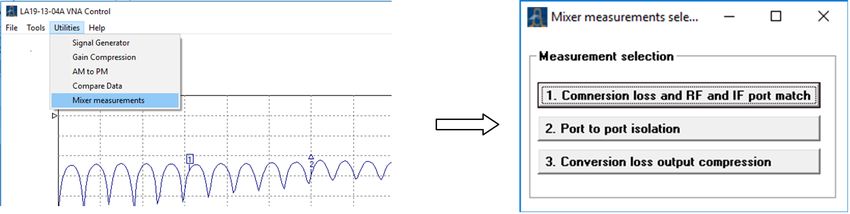
PicoVNA 6 and 8.5 GHz Vector Network Analyzers                                                               Safety

Power supply options and ratings
                                                                     Ext DC power supply
Model name              USB connection
                                                    Voltage                Current               Total power
PicoVNA 106                                                                                           22 W
                           USB 2.0.              12 to 15 V DC             1.85 A pk
PicoVNA 108                                                                                           25 W
                        Compatible with
SOLT-AUTO E-Cal            USB 3.0
                                                                                N/A
module

           WARNING
           Containment of radio frequencies
           The instrument contains a swept or CW radio frequency signal source (300 kHz to 6.02 GHz at +6
           dBm max. for the PicoVNA 106, 300 kHz to 8.50 GHz at +6 dBm max. for the PicoVNA 108) The
           instrument and supplied accessories are designed to contain and not radiate (or be susceptible to)
           radio frequencies that could interfere with the operation of other equipment or radio control and
           communications. To prevent injury or death, connect only to appropriately specified connectors,
           cables, accessories and test devices, and do not connect to an antenna except within approved test
           facilities or under otherwise controlled conditions.

1.5           Environment
           WARNING
           This product is suitable for indoor or outdoor use, in dry locations only. The product’s external mains
           power supply is for indoor use only
           WARNING
           To prevent injury or death, do not use the VNA or an accessory in wet or damp conditions, or near
           explosive gas or vapor.
           CAUTION
           To prevent damage, always use and store your VNA or accessory in appropriate environments.

                                          Storage                                       Operating
Temperature                           –20 to +50 °C                                    +5 to +40 °C
Humidity                                            20% to 80 %RH (non-condensing)
Altitude                                                         2000 m
Pollution degree                                                    2

           CAUTION
           Do not block the air vents at the back or underside of the instrument as overheating will cause
           damage.

           Do not insert any objects through the air vents as internal interference will cause damage.

pvug-5                              Copyright © 2017–2022 Pico Technology Ltd                                        4
PicoVNA 6 and 8.5 GHz Vector Network Analyzers                                                                Safety

1.6          Care of the product
The product and accessories contain no user-serviceable parts. Repair, servicing and calibration require
specialized test equipment and must only be performed by Pico Technology or an approved service provider.
There may be a charge for these services unless covered by the Pico three-year warranty.

            WARNING
            To prevent injury or death, do not use the VNA or accessory if it appears to be damaged in any way,
            and stop use immediately if you are concerned by any abnormal behavior.
            CAUTION
            Regularly inspect the instrument and all probes, connectors, cables and accessories before use for
            signs of damage or contamination.

            To prevent damage to the device or connected equipment, do not tamper with or disassemble the
            instrument, case parts, connectors, or accessories.

            When cleaning the product, use a soft cloth and a solution of mild soap or detergent in water, and do
            not allow liquids to enter the casing of the instrument or accessory.

            Take care to avoid mechanical stress or tight bend radii for all connected leads, including all coaxial
            leads and connectors. Mishandling will cause deformation of sidewalls, and will degrade
            performance. In particular, note that test port leads should not be formed to tighter than 5 cm (2”)
            bend radius.

            To prevent measurement errors and extend the useful life of test leads and accessory connectors,
            ensure that liquid and particulate contaminants cannot enter. Always fit the dust caps provided and
            use the correct torque when tightening. Pico recommends: 1 Nm (8.85 inch-lb) for supplied and all
            stainless steel connectors, or 0.452 Nm (4.0 inch-lb) when a brass or gold plated connector is
            interfaced.

pvug-5                               Copyright © 2017–2022 Pico Technology Ltd                                        5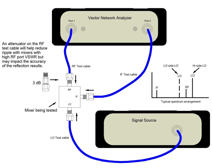
PicoVNA 6 and 8.5 GHz Vector Network Analyzers                                                    Quick start guide

2              Quick start guide
2.1            Installing the software
· Obtain the software from www.picotech.com/downloads:
  o PicoVNA 2 (for the PicoVNA 106 model)
  o PicoVNA 3 (for the PicoVNA 108 model)
· Connect the PicoVNA unit to the computer and wait while Windows automatically installs the driver.

In case of difficulties, refer to Software installation for more details.

Mixer measurements (PicoVNA 108 only)
Control of the PicoSource AS108 300 kHz to 8 GHz signal source is built into the PicoVNA software. If you wish to
carry out mixer measurements using other sources or sensors it is very likely that you will need to install the
Keysight® IO Libraries Suite to support communication with external instruments through either the USB or GPIB
interfaces. Please see www.keysight.com for details.

2.2            Loading the calibration kit(s)

For manual SOLT calibration:

·   Run the PicoVNA 2 or PicoVNA 3 software
·   In the main menu, select Tools > Calibration kit
·   Click Load P1 kit, select the data for your Port 1 kit and then click Apply
·   Click Load P2 kit, select the data for your Port 2 kit and then click Apply
Select the calibration kit(s) required depending on the device to be tested.
Note: If testing a non-insertable DUT with, for example, female connectors, use a single female kit for ports 1 and
2.

For the PicoVNA 108 and an automated calibration:

· Run the PicoVNA 3 software
· Connect the E-Cal module to a spare USB port on the controlling PC
· In the main menu, select Tools > Calibration kit

pvug-5                                 Copyright © 2017–2022 Pico Technology Ltd                                  6

PicoVNA 6 and 8.5 GHz Vector Network Analyzers                                                   Quick start guide

·   Click Electronic Cal kit
·   Select the E-Cal module and Port Adaptor arrangement to suit the test ports
·   Connect the E-Cal module, port adaptor and test ports to exactly match the selected configuration
·   Click Find and load EasyCal data
·   Upon completion select Exit
·   Then click Apply in the Calibration Kit Parameters menu

2.3           Setting up calibration parameters
· Click Calibration to open the Calibration window:

pvug-5                               Copyright © 2017–2022 Pico Technology Ltd                                  7
PicoVNA 6 and 8.5 GHz Vector Network Analyzers                                                      Quick start guide

2.4             Setting up display parameters
See Display Setup for details on using the mouse to set values.

· Click Display in the main window to open the Display Set Up window:

· When finished, click Start in the main window to begin measurements

2.5             Calibration tips
The bandwidth setting used during calibration largely determines the available dynamic range during the
measurement. The table below shows suggested bandwidth and power settings to use during calibration for
different types of measurement.

Measurement                Calibration     Calibration     Calibration   Comments
                           bandwidth       averaging         power
Fastest speed               10 kHz           None           +0 dBm       Set bandwidth to 140 kHz during
                                                                         measurement
Best accuracy and            100 Hz           None          –3 dBm       Leave bandwidth set to 100 Hz during
~100 dB dynamic range                                                    measurement
General use, fast speed,      1 kHz           None          +0 dBm       Leave bandwidth set to 1 kHz during
~90 dB dynamic range                                                     measurement
Best dynamic range            10 Hz           None          +6 dBm       Leave bandwidth set to 10 Hz during
                                                                         measurement. Refer to “Calibration for best
                                                                         dynamic range – minimizing the effect of
                                                                         crosstalk”.

2.6             Running in demo mode
Demo mode allows you to explore the user interface software with no instrument connected.

· To enter demo mode, run the PicoVNA 2 or PicoVNA 3 software with no instrument connected.
· For demo mode, click Ignore in the dialog that appears.

The software will then offer you a selection of demonstration measurements.

pvug-5                                Copyright © 2017–2022 Pico Technology Ltd                                        8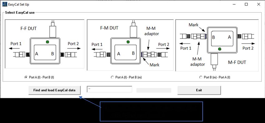
PicoVNA 6 and 8.5 GHz Vector Network Analyzers                                                       Description

3             Description
The PicoVNA 106 and 108 are PC-driven vector network analyzers capable of direct measurement of forward and
reverse parameters. The main characteristics are as follows:

Model                                PicoVNA 106                            PicoVNA 108
Operating frequency range            300 kHz to 6 GHz                       300 kHz to 8.5 GHz
Dynamic range                        ≤ 118 dB                               ≤ 124 dB
Frequency resolution                 ≤ 10 Hz                                ≤ 10 Hz

A simplified block diagram of the instrument is shown below:

              Simplified block diagram of the PicoVNA units

The architecture is based on a four-receiver (Quad RX) arrangement using a bandwidth of up to 140 kHz. Couplers
A and B are wideband RF bridge components which provide the necessary directivity in both directions. Signal
detection is by means of analog-to-digital converters used to sample the IF signal. The sample data is processed
by the embedded controller to yield the I and Q components. The detection system operates with an IF of 1.3 MHz
and employs a patented circuit technique to yield fast speeds with very low trace noise.

The instrument's software runs on a personal computer and communication with the instrument is through the
USB interface. The software carries out the mathematical processing and allows the display of measured
parameters in many forms, including:

·   frequency domain
·   time domain
·   de-embedding utility
·   measuring output power at the 1 dB gain compression point
·   measuring AM to PM conversion
·   measuring frequency mixer characteristics (PicoVNA 108 only)
·   measuring phase and amplitude alignment of two external signal sources (PicoVNA 108 only)

pvug-5                              Copyright © 2017–2022 Pico Technology Ltd                                  9
PicoVNA 6 and 8.5 GHz Vector Network Analyzers                                Description

                    Front panel of the PicoVNA 106 (PicoVNA 108 is similar)

                    Back panel of the PicoVNA 106 (PicoVNA 108 is similar)

pvug-5                        Copyright © 2017–2022 Pico Technology Ltd               10
PicoVNA 6 and 8.5 GHz Vector Network Analyzers Description
SOLT-STD-M/F and SOLT-PREM-M/F manual calibration standards
SOLT-AUTO-M/F automatic (E-Cal) calibration standards
pvug-5 Copyright © 2017–2022 Pico Technology Ltd 11PicoVNA 6 and 8.5 GHz Vector Network Analyzers Vector network analyzer basics
4 Vector network analyzer basics
4.1 Introduction
A vector network analyzer is used to measure the performance of circuits or networks such as amplifiers, filters,
attenuators, cables and antennas. It does this by applying a test signal to the network to be tested, measuring the
reflected and transmitted signals and comparing them to the test signal. The vector network analyzer measures
both the magnitude and phase of these signals.
4.2 Structure of the VNA
The VNA consists of a tunable RF source, the output of which is split into two paths. The signal feeds to the
couplers are each measured by their respective reference receivers through power dividers. In the forward mode,
the test signal is passed through a directional coupler or directional bridge before being applied to the DUT. The
directional output of the coupler, which selects only signals reflected from the input of the DUT, is connected to
the Port1 receiver where the signal’s magnitude and phase are measured. The rest of the signal, the portion that
is not reflected from the input, passes through the DUT to the Port2 receiver where its magnitude and phase are
measured. The measurements at the Port1 and Port2 receivers are referenced to the measurements made by the
Ref1 and Ref2 receivers so that any variations due to the source are removed. The Ref1 and Ref2 receivers also
provide a reference for the measurement of phase.
Simplified vector network analyzer block diagram
In reverse mode, the test signal is applied to the output of the DUT, and the Port2 receiver is used to measure the
reflection from the output port of the DUT while the Port1 receiver measures the reverse transmission through the
DUT.
4.3 Measurement
Vector network analyzers have the capability to measure phase as well as magnitude. This is important for fully
characterizing a device or network either for verifying performance or for generating models for design and
simulation. Knowledge of the phase of the reflection coefficient is particularly important for matching systems
for maximum power transfer. For complex impedances the maximum power is transferred when the load
impedance is the complex conjugate of the source impedance (see figure).
pvug-5 Copyright © 2017–2022 Pico Technology Ltd 12PicoVNA 6 and 8.5 GHz Vector Network Analyzers Vector network analyzer basics
Matching a load for maximum power transfer
Measurement of phase in resonators and other components is important in designing oscillators. In feedback
oscillators, oscillation occurs when the phase shift round the loop is a multiple of 360° and the gain is unity. It is
important that these loop conditions are met as close as possible to the center frequency of the resonant
element to ensure stable oscillation and good phase noise performance.
The ability to measure phase is also important for determining phase distortion in a network. Phase distortion can
be important in both analog and digital systems. In digital transmission systems, where the constellation depends
on both amplitude and phase, any distortion of phase can have serious effects on the errors detected.
4.4 S-parameters
The basic measurements made by the vector network analyzer are S (scattering) parameters. Other parameters
such as H, Y, T and Z parameters may all be deduced from the S-parameters if required. The reason for
measuring S-parameters is that they are made under conditions that are easy to produce at RF. Other parameters
require the measurement of currents and voltages, which is difficult at high frequencies. They may also require
open circuits or short circuits that can be difficult to achieve at high frequencies, and may also be damaging to
the device under test or may cause oscillation.
Forward S-parameters are determined by measuring the magnitude and phase of the incident, reflected and
transmitted signals with the output terminated with a load that is equal to the characteristic impedance of the test
system (see figure below).
pvug-5 Copyright © 2017–2022 Pico Technology Ltd 13PicoVNA 6 and 8.5 GHz Vector Network Analyzers Vector network analyzer basics
S-parameter definitions
pvug-5 Copyright © 2017–2022 Pico Technology Ltd 14PicoVNA 6 and 8.5 GHz Vector Network Analyzers Vector network analyzer basics
The measured parameters are presented in a file similar to the one below. The format is as follows:
· Header lines: these start with a ! symbol and give general information such as time and date.
· Format line: this starts with a # symbol and gives information about the format of the data.
o First field gives the frequency units, in this case MHz
o Second field indicates the parameters measured, in this case S-parameters
o Third field indicates the format of the measurement, in this case MA meaning magnitude and angle. Others
formats are RI, meaning real and imaginary, and DB, meaning log magnitude and angle.
· Data lines. The number of columns of data depends on the parameters that have been measured.
o A 1-port measurement measures the reflected signal from the device under test and usually produces three
columns. If the format is MA (magnitude and angle), the first column is the measurement frequency, the
second is the magnitude of S11 and the third is the angle of S11. If the format is RI, the second column is the
real part of S11 and the third column is the imaginary part of S11.
o When a reflection and transmission measurement is made there are five columns of data. Column 1 is the
measurement frequency, columns 2 and 3 contain S11 magnitude and angle or real and imaginary data, and
columns 4 and 5 contain S21 magnitude and angle or real and imaginary data.
o If a full 2-port measurement is made, there will be nine columns of data. Column 1 contains frequency
information, columns 2 and 3 S11 data, 4 and 5 S21 data, 6 and 7 S12 data, and 8 and 9 S22 data.
The PicoVNA 106 and 108 can generate full set of 2-port parameters but you can choose to export either 1-port
.s1p or full 2-port .s2p S-parameter files to suit most RF and microwave circuit simulators.
Part of a typical 2-port S-parameter file is shown below. The header shows that the frequency units are MHz, the
data format is Magnitude and Angle and the system impedance is 50 Ω. Column 1 shows frequency, 2 and 3 S11,
4 and 5 S21, 6 and 7 S12, and 8 and 9 S22.
! 06/09/2005 15:47:34
! Ref Plane: 0.000 mm
# MHZ S MA R 50
!
3 0.00776 16.96 0.99337 -3.56 0.99324 -3.53 0.00768 12.97
17.985 0.01447 19.99 0.9892 -20.80 0.98985 -20.72 0.01519 15.23
32.97 0.01595 20.45 0.98614 -37.96 0.98657 -37.95 0.01704 6.40
47.955 0.01955 28.95 0.98309 -55.15 0.98337 -55.10 0.018 1.75
62.94 0.02775 24.98 0.98058 -72.29 0.98096 -72.29 0.0199 -6.07
77.925 0.03666 11.76 0.97874 -89.46 0.9803 -89.45 0.02169 -23.06
92.91 0.04159 -6.32 0.97748 -106.62 0.9786 -106.62 0.01981 -48.43
107.895 0.0426 -24.79 0.97492 -123.77 0.97579 -123.89 0.01424 -87.79
122.88 0.0396 -41.35 0.97265 -141.25 0.97269 -141.30 0.00997 -166.81
137.865 0.03451 -52.96 0.96988 -158.65 0.96994 -158.76 0.01877 113.15
152.85 0.03134 -56.07 0.96825 -176.27 0.96858 -176.28 0.03353 69.81
167.835 0.03451 -57.72 0.96686 166.10 0.96612 165.99 0.04901 34.83
182.82 0.04435 -67.59 0.9639 148.18 0.96361 148.21 0.06131 1.42
197.805 0.05636 -86.28 0.96186 130.15 0.96153 130.06 0.07102 -33.33
212.79 0.06878 -110.45 0.95978 111.82 0.95996 111.90 0.07736 -69.57
227.775 0.08035 -136.14 0.9557 93.50 0.9568 93.41 0.08303 -107.21
242.76 0.09099 -161.24 0.95229 74.84 0.95274 74.89 0.08943 -144.34
257.745 0.10183 175.34 0.94707 56.03 0.94755 55.95 0.09906 -179.63
pvug-5 Copyright © 2017–2022 Pico Technology Ltd 15PicoVNA 6 and 8.5 GHz Vector Network Analyzers Vector network analyzer basics
4.5 Displaying measurements
Input and output parameters, S11 and S22, are often displayed on a polar plot or a Smith chart. The polar plot
shows the result in terms of the complex reflection coefficient, but impedance cannot be directly read off the
chart. The Smith chart maps the complex impedance plane onto a polar plot. All values of reactance and all
positive values of resistance, from 0 to ∞, fall within the outer circle. This has the advantage that impedance
values can be read directly from the chart.
The Smith chart
pvug-5 Copyright © 2017–2022 Pico Technology Ltd 16PicoVNA 6 and 8.5 GHz Vector Network Analyzers Vector network analyzer basics
4.6 Calibration and error correction
Before accurate measurements can be made, the network analyzer needs to be calibrated. In the calibration
process, well-defined standards are measured and the results of these measurements are used to correct for
imperfections in the hardware. The most common calibration method, SOLT (short, open, load, thru), uses four
known standards: a short circuit, an open circuit, a load matched to the system impedance, and a through line.
These standards are usually contained in a calibration kit and their characteristics are stored on the controlling
PC in a Cal Kit definition file. Analyzers such as the PicoVNA 106 and 108 that have a full S-parameter test set can
measure and correct all 12 systematic error terms.
Six key sources of errors in forward measurement.
Another six sources exist in the reverse measurement (not shown).
pvug-5 Copyright © 2017–2022 Pico Technology Ltd 17PicoVNA 6 and 8.5 GHz Vector Network Analyzers Vector network analyzer basics 4.7 Other measurements S-parameters are the fundamental measurement performed by the network analyzer, but many other parameters may be derived from these including H, Y and Z parameters. 4.7.1 Reflection parameters The input reflection coefficient Γ can be obtained directly from S11: ρ is the magnitude of the reflection coefficient i.e. the magnitude of S11: ρ = |S11| Sometimes ρ is expressed in logarithmic terms as return loss: return loss = –20 log(ρ) VSWR can also be derived: VSWR definition 4.7.2 Transmission parameters Transmission coefficient T is defined as the transmitted voltage divided by the incident voltage. This is the same as S21. If T is less than 1, there is loss in the DUT, which is usually referred to as insertion loss and expressed in decibels. A negative sign is included in the equation so that the insertion loss is quoted as a positive value: If T is greater than 1, the DUT has gain, which is also normally expressed in decibels: pvug-5 Copyright © 2017–2022 Pico Technology Ltd 18
PicoVNA 6 and 8.5 GHz Vector Network Analyzers                                        Vector network analyzer basics

4.7.3         Phase
The phase behavior of networks can be very important, especially in digital transmission systems. The raw phase
measurement is not always easy to interpret as it has a linear phase increment superimposed on it due to the
electrical length of the DUT. Using the reference plane function the electrical length of the DUT can be removed
leaving the residual phase characteristics of the device.

                            Operation on phase data to yield underlying characteristics

4.7.4         Group delay
Another useful measurement of phase is group delay. Group delay is a measure of the time it takes a signal to
pass through a network versus frequency. It is calculated by differentiating the phase response of the device
with respect to frequency, i.e. the rate of change of phase with frequency:

The linear portion of phase is converted to a constant value typically, though not always, representing the average
time for a signal to transit the device. Differences from the constant value represent deviations from linear phase.
Variations in group delay will cause phase distortion as a signal passes through the circuit.

When measuring group delay the aperture must be specified. Aperture is the frequency step size used in the
differentiation. A small aperture will give more resolution but the displayed trace will be noisy. A larger aperture
effectively averages the noise but reduces the resolution.

pvug-5                                 Copyright © 2017–2022 Pico Technology Ltd                                       19
PicoVNA 6 and 8.5 GHz Vector Network Analyzers Vector network analyzer basics
4.7.5 Gain compression
The 1 dB gain compression point of amplifiers and other active devices can be measured using the power sweep.
The small signal gain of the amplifier is determined at low input power, then the power is increased and the point
at which the gain has fallen by 1 dB is noted.
The 1 dB gain compression is often used to quote output power capability.
4.7.6 AM to PM conversion
Another parameter that can be measured with the VNA is AM to PM conversion. This is a form of signal distortion
where fluctuations in the amplitude of a signal produce corresponding fluctuations in the phase of the signal.
This type of distortion can have serious effects in digital modulation schemes where both amplitude and phase
accuracy are important. Errors in either phase or amplitude cause errors in the constellation diagram.
4.7.7 Time domain reflectometry (TDR)
Time domain reflectometry is a useful technique for measuring the impedance of transmission lines and for
determining the position of any discontinuities due to connectors or damage. The network analyzer can determine
the time domain response to a step input from a broad band frequency sweep at harmonically related
frequencies. An inverse Fourier Transform is performed on the reflected frequency data (S11) to give the impulse
response in the time domain. The impulse response is then integrated to give the step response. Reflected
components of the step excitation show the type of discontinuity and the distance from the calibration plane.
A similar technique is used to derive a TDT (Time Domain Transmission) signal from the transmitted signal data
(S21). This can be used to measure the rise time of amplifiers, filters and other networks. The following provides
a more detailed treatment of TDR and TDT.
pvug-5 Copyright © 2017–2022 Pico Technology Ltd 20PicoVNA 6 and 8.5 GHz Vector Network Analyzers Vector network analyzer basics 4.7.7.1 Traditional TDR The traditional TDR consists of a step source and sampling oscilloscope (see figure below). A step signal is generated and applied to a load. Depending on the value of the load, some of the signal may be reflected back to the source. The signals are measured in the time domain by the sampling scope. By measuring the ratio of the input voltage to the reflected voltage, the impedance of the load can be determined. Also, by observing the position in time when the reflections arrive, it is possible to determine the distance to impedance discontinuities. Traditional TDR setup 4.7.7.1.1 Example: shorted 50 ohm transmission line Simplified representation of the response of a shorted line. pvug-5 Copyright © 2017–2022 Pico Technology Ltd 21
PicoVNA 6 and 8.5 GHz Vector Network Analyzers                                       Vector network analyzer basics

For a transmission line with a short circuit (figure above) the incident signal sees the characteristic impedance of
the line so the scope measures Ei. The incident signal travels along the line to the short circuit where it is
reflected back 180° out of phase. This reflected wave travels back along the line canceling out the incident wave
until it is terminated by the impedance of the source. When the reflected signal reaches the scope the signal
measured by the scope goes to zero as the incident wave has been canceled by the reflection. The result
measured by the scope is a pulse of magnitude Ei and duration that corresponds to the time it takes the signal to
pass down the line to the short and back again. If the velocity of the signal is known, the length of the line can be
calculated:

where v is the velocity of the signal in the transmission line, t is the measured pulse width and d is the length of
the transmission line.

4.7.7.1.2     Example: open-circuited 50 ohm transmission line

  Simplified representation of the response of a open line

In the case of the open circuit transmission line (figure above) the reflected signal is in phase with the incident
signal, so the reflected signal combines with the incident signal to produce an output at the scope that is twice
the incident signal. Again, the distance d can be calculated if the velocity of the signal is known.

4.7.7.1.3     Example: resistively terminated 50 ohm transmission line

  Simplified representation of the response of a resistively terminated line

pvug-5                                Copyright © 2017–2022 Pico Technology Ltd                                        22
PicoVNA 6 and 8.5 GHz Vector Network Analyzers                                     Vector network analyzer basics

4.7.7.1.4     Reactive terminations and discontinuities
Reactive elements can also be determined by their response. Inductive terminations produce a positive pulse.
Capacitive terminations produce a negative pulse.

  Simplified representation of the response of a reactively terminated line

Similarly, the position and type of discontinuity in a cable, due to connectors or damage, can be determined. A
positive pulse indicates a connector that is inductive or damage to a cable, such as a removal of part of the outer
screen. A negative-going pulse indicates a connector with too much capacitance or damage to the cable, such as
being crushed.

  Simplified representation of the response of a line discontinuity

4.7.7.2       Time domain from frequency domain
An alternative to traditional TDR is where the time domain response is determined from the frequency domain
using an Inverse Fast Fourier Transform (IFFT). Several methods are available for extracting time domain
information from the frequency domain. The main methods are lowpass and bandpass.

4.7.7.2.1     Lowpass method
The lowpass method can produce results that are similar to the traditional TDR measurements made with a time
domain reflectometer using a step signal, and can also compute the response to an impulse. It provides both
magnitude and phase information and gives the best time resolution. However, it requires that the circuit is DC-
coupled. This is the method supported by the PicoVNA 106 and 108.

pvug-5                               Copyright © 2017–2022 Pico Technology Ltd                                   23
PicoVNA 6 and 8.5 GHz Vector Network Analyzers                                       Vector network analyzer basics

The lowpass method uses an Inverse Fourier Transform to determine the impulse response in the time domain
from the reflection coefficient measured in the frequency domain. The DC component is extrapolated from the
low-frequency data to provide a phase reference. Alternatively, if the DC termination is known it can be entered
manually. Once the impulse response is computed, the step response may be determined from the time integral
of the impulse response. In the step response mode the trace is similar to that of a TDR, except that there is no
step at t = 0. When the time domain response is derived from the frequency information the value at t = 0 is the
impedance of the transmission line or load immediately following the calibration plane. The value is referenced to
50 Ω, the characteristic impedance of the system. For example, an open circuit would appear as a value of +1 unit
relative to the reference value and a short circuit would appear as a value of –1 unit relative to the reference value
(see example TDR plots above).

To facilitate the use of the Inverse Fourier Transform to compute the time domain response, the samples in the
frequency domain must be harmonically related and consist of 2n points. For this reason, the TDR facility in the
PicoVNA 106 and 108 makes available special 512, 1024, 2048 and 4096-frequency-point calibrations with a stop
frequency of up to 6000 MHz (PicoVNA 106) or 8500 MHz (PicoVNA 108). The resulting alias-free range is a
function of the number of frequency points (N) and the total frequency span. It is given by the expression:

So, the available ranges on the PicoVNA units are approximately as follows:

Model                                  PicoVNA 106                            PicoVNA 108
Ranges                                 100 ns, 171 ns, 341 ns, 683 ns         60 ns, 120 ns, 240 ns, 481 ns
Time resolution                        98 ps to 84 ps                         58 ps

The transform returns twice the number of points of the calibration in the time domain. Therefore the above
ranges provide time resolutions approximately as shown.

4.7.7.2.2     Bandpass method
The bandpass method provides only magnitude information so it is not possible to distinguish between inductive
and capacitive reactances. Also, the time resolution is only half as good as in the lowpass mode. However, the
method can be used for circuits where there is no DC path and hence is suitable for AC-coupled circuits such as
bandpass filters. This method is not currently supported by the PicoVNA 106 and 108.

4.7.7.3       Windowing
The bandwidth of the network analyzer is limited by the frequency range, so the frequency domain data will be
truncated at the bandwidth of the analyzer. Also the analyzer gathers data at discrete frequencies. The result of
the sampled nature of the data and the truncation in the frequency domain is to produce a sin(x)/x response when
transformed to the time domain. This appears as ringing on both the displayed impulse response and the step
response. To overcome this problem, a technique known as windowing can be applied to the frequency domain
data before implementing the Inverse Fourier Transform.

The windowing function progressively reduces the data values to zero as the edge of the frequency band is
approached, thus minimizing the effect of the discontinuities. When the modified data is transformed, the ringing
is reduced or removed depending on the selected windowing function. However, the windowing function reduces
the bandwidth and so increases the width of the pulse in impulse response mode and slows the edge in step
response mode. A balance must be made between the width of the pulse, or speed of the edge, and the amount
of ringing to be able to determine closely spaced discontinuities. The PicoVNA 106 and 108 allow you to choose a
rectangular window (no bandwidth reduction), a Hanning window (raised cosine), or a Kaiser–Bessel window.
The order of the Kaiser–Bessel window is configurable.

pvug-5                                Copyright © 2017–2022 Pico Technology Ltd                                     24
PicoVNA 6 and 8.5 GHz Vector Network Analyzers                                  Vector network analyzer basics

4.7.7.4       Aliasing
The sampled nature of the data means it is subject to the effects of aliasing. The result is repetition of time-
domain response at the effective sampling rate in the frequency domain. This limits the maximum time delay and
hence maximum cable length that can be observed. In the PicoVNA 106 this is 683 ns (approximately 138 m of
cable) and in the PicoVNA 108 it is 481 ns (approximately 97 m of cable).

pvug-5                              Copyright © 2017–2022 Pico Technology Ltd                                 25
PicoVNA 6 and 8.5 GHz Vector Network Analyzers                                                      Getting started

5              Getting started
Refer to the Quick Start Guide above for initial instructions, then return here for more detail.

5.1            Minimum requirements
A PC or laptop is required to operate the VNA. The recommended minimum requirements are stated in the
Specifications.

The performance of the software is influenced by the performance of the PC and video adaptor installed in it. It is
important that an adaptor with good graphics performance is used. As a general guide, it is recommended that an
adaptor with at least 64 MB of memory is used.

5.2            Software installation
Follow the Quick Start Guide to install the software from the disk or from www.picotech.com. The installer will
copy the program and the USB driver to your computer. You need administrative privileges in order to run the
installer.

The installer creates a support directory at one of these locations:

· PicoVNA 106: C:\User\Public\Documents\PicoVNA2
· PicoVNA 108: C:\User\Public\Documents\PicoVNA3

This directory contains the following files:

·   xxx-log.txt             The status log file. ‘xxx’ is the serial number
·   DefCal.cal              Default calibration data (last used calibration)
·   UsersGuide.pdf          This User's Guide
·   Support\                Folder with data files to support the software

5.2.1          Typical error messages
On Windows 7 machines it is common to see the following error message:

It is safe to click Ignore to continue the installation.

pvug-5                                  Copyright © 2017–2022 Pico Technology Ltd                                 26
PicoVNA 6 and 8.5 GHz Vector Network Analyzers                                                    Getting started

5.2.2         Mixer measurements (PicoVNA 108 only)
Control of the PicoSource AS108 300 kHz to 8 GHz signal source is built into the PicoVNA software. If you wish to
carry out mixer measurements using other sources or sensors it is very likely that you will need to install the
Keysight® IO Libraries Suite to support communication with external instruments through either the USB or GPIB
interfaces. Please see www.keysight.com for details.

pvug-5                               Copyright © 2017–2022 Pico Technology Ltd                                 27
PicoVNA 6 and 8.5 GHz Vector Network Analyzers                                                         Getting started

5.3           Switching on the VNA
When the VNA is powered on, the front-panel channel activity indicators will flash to indicate that the controller
has started correctly.

5.4           Calibration kit parameters
The minimum requirements to carry out a 12-term calibration (full error correction) depend on the device to be
tested. For example, the most accurate calibration is for insertable devices, and this requires a total of six
standards: three of the four in each of the male and female cal standards.

An ‘insertable’ device is one that has connectors of different sexes at its ports. On the other hand, a calibration
for a non-insertable device can be carried out using only three standards by using the unknown thru calibration
method.

The calibration kits parameters can be inspected using the Calibration Kit Parameters window (see below) found
under the Tools menu. From this the kit editor can be launched to modify and create new kits as discussed later
in the section.

The unknown thru calibration method only requires that the thru adaptor be reciprocal: that is, have S21 = S12.

                           Calibration Kit window. The short/open offsets are in mm in air.

5.4.1         Manual fixed SOLT calibration - insertable DUT
Two Pico calibration kits required: Premium PC3.5 kits SOLT-PREM-M and SOLT-PREM-F or Standard SMA kits
SOLT-STD-M and SOLT-STD-F or alternative calibration kits comprising:

· Open circuit (2 pieces, one male and one female)
· Short circuit (2 pieces, one male and one female)
· Matched termination (2 pieces, one male and one female)

pvug-5                                Copyright © 2017–2022 Pico Technology Ltd                                       28
PicoVNA 6 and 8.5 GHz Vector Network Analyzers Getting started
For insertable DUTs the requirement is for two calibration kits, one of each sex. Generally, it is required that the
matched termination should be of good quality and, as a guide, should have a return loss of better than 40 dB.
However, the PicoVNA 106 and 108 allow terminations with relatively poor return loss values to be used and still
maintain good accuracy. This is discussed in Using a matched termination.
5.4.2 Manual fixed SOLT calibration - non-insertable DUT
One Pico calibration kit required: Premium PC3.5 kit SOLT-PREM-M or SOLT-PREM-F or Standard SMA kits
SOLT-STD-M or SOLT-STD-for alternative calibration kit comprising:
· Open circuit (1 piece)
· Short circuit (1 piece)
· Matched termination (1 piece)
· Either a characterized through connection adaptor (1 piece) or any uncharacterized reciprocal adaptor
For non-insertable DUTs only a single calibration kit is required. In addition, a reciprocal but otherwise unknown
thru adaptor, or a fully characterized thru adaptor, is required. The latter is supplied with all Pico standard kits.
5.4.3 Open circuit model
The open circuit capacitance model used is described by the equation below, where F is the operating frequency.
Generally, with typical open circuit standards, the effect is small, amounting to no more than a few degrees of
phase shift at 6 or 8.5 GHz.
Copen = C0 + C1F + C2F2 + C3F3
In addition, an offset length (sometimes referred to as offset delay) can be entered as well as the loss of the
offset line.
5.4.4 Short circuit model
The short circuit inductance is modeled by an inductance component and in addition, a non-zero offset length can
be entered together with the loss of the offset line.
5.4.5 Short and open without models
The PicoVNA 106 and 108 support short and open standards defined by data only. In this case the data is
supplied in the form of a 201-frequency-points table. Each frequency point has three comma-separated entries:
frequency (in MHz), real part of the reflection coefficient and the imaginary part of the reflection coefficient.
5.4.6 Calibration kit editor
As already mentioned, the calibration kit editor can be used to create or edit an existing calibration kit. The figure
below shows the editor window. A typical example is to create a new kit using an existing kit as a template to
speed the process. So, the process would be to first load the existing calibration kit from the Calibration Kit
Parameters window. Type the new kit name in the name box and modify the parameters as needed. Finally, click
Save Kit to save the new kit with a new name.
In the above example, if the existing kit loaded had load data or through data and you want to replace this with
new data, uncheck the appropriate box and then check it again.
pvug-5 Copyright © 2017–2022 Pico Technology Ltd 29PicoVNA 6 and 8.5 GHz Vector Network Analyzers Getting started
Calibration Kit Editor
The calibration kits optionally supplied with the PicoVNA 106 and 108 provide an economical solution while
retaining good measurement accuracy. They are supplied with SMA or precision PC3.5 (SMA-compatible)
connectors. Refer to the PicoVNA 100 Series Data Sheet for details.
5.4.7 Using a matched termination with poor return loss or
unmodeled short and open
A successful calibration can be carried out without the need for a good-quality matched load. In order to retain
accuracy, it is necessary to provide the instrument with accurate performance data of the matched load to be
used. The data needs to be in a fixed format thus:
Frequency (MHz) S11 (real) S11 (imaginary)
1.0 -1.7265E-03 7.7777E-05 There must be 201 data lines. Typically these
30.995 -1.6588E-03 3.3093E-04 should cover the band 0.3 MHz to (6.00 GHz or
8.50 GHz). No empty or comment lines are
60.99 -1.4761E-03 5.9003E-04
allowed.
90.985 -1.4653E-03 1.0253E-03
120.98 -1.3841E-03 1.2608E-03
150.975 -1.1924E-03 1.5800E-03
240.96 -1.0884E-03 1.9085E-03
300.95 -8.7216E-04 2.1355E-03
330.945 -7.0326E-04 2.4109E-03
360.94 -5.7006E-04 2.6790E-03
Format for characteristics of matched load
In the case when the models for the open and short are not known, it is possible to enter measured data in the
same format as shown above. This approach can give good results if the open and short can be measured
accurately, particularly at the higher frequencies where it is usually difficult to model components accurately.
When supplied, the data for the through connection adaptor must be in the format shown below. The data must
be a full set of S-parameters with no empty or comment lines. It is important that the data spans as much of the
full frequency range as possible, for example from 0.3 MHz to (6000 MHz or 8500 MHz).
pvug-5 Copyright © 2017–2022 Pico Technology Ltd 30PicoVNA 6 and 8.5 GHz Vector Network Analyzers Getting started Freq (MHz) S11r S11i S21r S21i S12r S12i S22r S22i 0.3 1.1450E-04 -1.0852E-04 0.9965E-01 -1.0394E-03 9.9947E-01 -7.4717E-04 1.0723E-04 4.9711E-05 40.3 2.9307E-04 1.9923E-04 9.9973E-01 -1.0241E-02 9.9934E-01 -1.0505E-02 2.0715E-04 2.0814E-04 80.3 4.1774E-04 4.3168E-04 9.9922E-01 -1.9672E-02 9.9927E-01 -1.9668E-02 2.8195E-04 2.8897E-04 120.3 5.3415E-04 5.7609E-04 9.9898E-01 -2.9165E-02 9.9855E-01 -2.8852E-02 4.0525E-04 2.8043E-04 160.3 7.1924E-04 6.4942E-04 9.9883E-01 -2.9165E-02 9.9855E-01 -2.8852E-02 4.0646E-04 2.8133E-04 200.3 7.8941E-04 7.5903E-04 9.9834E-01 -3.8214E-02 9.9846E-01 -3.8128E-02 5.4323E-04 2.2344E-04 240.3 9.9069E-04 7.8162E-04 9.9792E-01 -5.7033E-02 9.9758E-01 -4.7805E-02 5.7273E-04 2.9411E-04 280.3 1.0791E-03 8.0397E-04 9.9715E-01 -6.6419E-02 9.9699E-01 -6.5967E-02 5.7191E-04 2.6551E-04 320.3 1.2779E-03 8.5429E-04 9.9648E-01 -7.5557E-02 9.9625E-01 -7.5449E-02 6.3081E-04 2.9580E-04 ... and so on, to a total of 201 frequency points Format for the characteristics of the through connector. These must be a full set of S-parameters (real and imaginary). To add matched load, short and open, or thru adaptor data to a calibration kit, follow the steps below: · Load kit using the Kit Editor (see Calibration Kit) · Check the Load Data Available box and similarly the boxes for the Thru and Short and Open circuits in the Kit Editor parameters window. · If the existing kit already has load, short and open, or through data, uncheck and recheck the appropriate box. If this is not done, the existing data will be kept and copied to the new kit. · If needed, manually enter the rest of the kit parameters. Ensure that the correct offset is entered. · Click Save Kit · When prompted, select the data file containing the matched load or the thru adaptor data in the format shown above. · Save the kit for future use by clicking the Save Kit button (see Calibration Kit). Note: When a kit is loaded, any available matched load or thru adaptor data that is associated with the kit will be automatically loaded. The calibration kits available for the PicoVNA 106 and 108 come complete with matched load, short and open, and thru adaptor data. Copy these files to your computer for easy access. It is critically important that the correct kit data, with the correct serial number, is loaded. 5.4.8 Using a third-party calibration kit The PicoVNA 106 and 108 may be used with third-party calibration kits, such as the Keysight/Agilent 85032F, that are characterized by polynomial coefficient models either in written form or as a text file. 1. Use the PicoVNA cal kit editor (Tools > Calibration Kit > Cal Kit Editor). 2. Uncheck all the "data available" boxes. 3. Enter the four poly coefficients of Open capacitance. 4. Enter only the L0 poly coefficient of Short inductance (neglecting the small and HF dominating coefficients) 5. Enter the Short and Open Loss terms. 6. Convert Short and Open offset times (ps) to distance (mm) in air and enter those. 7. The short and open Z0 values are not used (assumed 50 Ω). 8. Nothing is entered for the Load. 9. As this Cal Kit does not have a Thru, we have left the length as zero. If a Thru is provided, measure the length (reference plane to reference plane in mm) and enter that to recreate these files. pvug-5 Copyright © 2017–2022 Pico Technology Ltd 31
PicoVNA 6 and 8.5 GHz Vector Network Analyzers                                                       Getting started

10. Save the cal kit file(s) generated by the editor. We suggest including the calibration kit model number, and
serial number if provided, in the file name.

5.4.9         Defining and Using TRL/TRM Calibration Standards
              (PicoVNA 108 Only)
Below is a summary explanation of preparation for a TRL/TRM calibration. Further detail can be gained from the
white paper entitled TRL calibration for SMT devices using the PicoVNA 108.

Higher Frequencies - Reference line length
For the TRL calibration of higher frequencies it is generally recommended that the line length, ΔL, is selected to
provide no less than 20º and no more than 160º of phase shift with respect to the thru length over the band of
operation. In practice, best results are achieved by restricting the range to around 30º to 150º.
The required reference line length can be calculated as follows.

Φ = phase shift in degrees
f = frequency
c = speed of light
εeff = effective dielectric constant

It is sensible to avoid lower microwave frequencies in order to avoid skin depth effects. So, keeping to 1.5 or 2
GHz and above may be a good idea.

Note: The absolute value of L is not important.
However, all L/2 sections shown must be identical and be exactly half the value of L.

pvug-5                                 Copyright © 2017–2022 Pico Technology Ltd                                     32
PicoVNA 6 and 8.5 GHz Vector Network Analyzers Getting started
PCB circuit blocks for TRL calibration and measurement
For example, assuming a nominal 50 Ω line with resulting effective dielectric constant of 3.35, to achieve 30º
phase shift at, say, 1.5 GHz, we find that:
∆L = 9.1 mm
This reference line length of 9.1 mm would in turn provide 150º of phase shift at 7.5 GHz. So, the useable
bandwidth for this line, as a TRL line standard, is 1.5 GHz to 7.5 GHz.
Lower frequencies - Matched Loads for TRM calibration
The PicoVNA 108 automatically switches to TRM at frequencies below those supported by the TRL reference
line(s). The TRM technique relies on matched loads to set the reference impedance. This approach works well
since good matched loads can easily be implemented at lower microwave frequencies (< 2 GHz). The frequency
range of the TRL reference line is set in the calibration kit definition and is described in the following section.
TRL calibration kit
In order to perform a TRL calibration with the PicoVNA 108, a calibration kit file needs to be created. This can be
done very easily using the calibration kit editor (Tools > Calibration kit > Cal Kit Editor).
Use the calibration kit editor to create the TRL cal kit file
TRL calibration kit – entering the reference line information
In this example we will use only one of the possible reference lines (‘Delays’) so we check just the box next to
‘Line 1’ to indicate that the cal kit has only one reference line. The Line 2 box is left unchecked as shown above.
We can either enter the electrical delay in ps and click the button Compute from delay to set the frequency range
of the line, or preferably, enter directly a narrower frequency range we wish to assign to the reference line. The
low frequency is entered into the box labeled FL and the high frequency into the box FH. Both values are in GHz.
pvug-5 Copyright © 2017–2022 Pico Technology Ltd 33PicoVNA 6 and 8.5 GHz Vector Network Analyzers Getting started TRL calibration kit – entering the Reflect Standard information The next step is to select whether the Reflect Standard is going to be a short or an open circuit. Click the appropriate radio button as required. Note that it is only necessary to know approximately the value of the reflection coefficient of the Reflect Standard. So, for example we could use on-PCB short circuits implemented with vias to ground. For this, we can enter 100 pH as an approximate value of the inductance into the box labeled L (pH). Alternatively a more accurate value might be available from design CAD or direct measurement. Likewise if we chose to use Open reflection standards we would enter a capacitance value at C0. Finally, we enter the desired Kit name in the top left box and click Save Kit to save the file to disk. We would recommend indication of this being a TRL Kit with Open/Short reflect standards and possibly its Max frequency coverage within the file name. pvug-5 Copyright © 2017–2022 Pico Technology Ltd 34
PicoVNA 6 and 8.5 GHz Vector Network Analyzers                                                           Operation

6             Operation
The PicoVNA 2 and PicoVNA 3 software allows you to program the measurement parameters and plots the
measurement results in real time. The main window includes a status panel that displays information including
calibration status, frequency sweep step size and sweep status. The Help menu includes a copy of this manual.

6.1           The PicoVNA 2 or 3 main window
The PicoVNA 2 main window is shown below. PicoVNA 3 is similar. It is dominated by a large graphics area where
the measurement results are plotted together with the readout of the markers. One, two or four plots can be
displayed simultaneously. The plots can be configured to display the desired measurements.

                                             User interface window

6.1.1         Display setup
Setting up the display is carried out through the Display Set Up window which is called up from the main window
by clicking Display. The window is shown below. The typical sequence to set up the display is as follows:

· Set the number of channels to be displayed by clicking the appropriate radio button under Display Channels
· Select the desired active channel from the drop-down list (can also be selected by clicking on a marker in the
  main window on the desired display channel)
· Select the channel to set up by clicking the appropriate radio button under Select

pvug-5                               Copyright © 2017–2022 Pico Technology Ltd                                     35
PicoVNA 6 and 8.5 GHz Vector Network Analyzers Operation
· Choose the desired parameter to display on this channel from the drop-down list under Parameter / Graph
Type
· Choose the desired graph type from the drop-down list under Parameter / Graph Type
· Select the vertical axis values from the Vertical Axis section. Optionally, click Autoscale to automatically set
the sensitivity and reference values. Note that reference position 1 is at the top (see second figure below).
· Click Apply to apply the selected values
· Repeat the above steps for each display needed
Note: The Active Channel must be one of the displayed channels.
The Display Set Up window is used to set up the measurements display
Display graph parameters
pvug-5 Copyright © 2017–2022 Pico Technology Ltd 36PicoVNA 6 and 8.5 GHz Vector Network Analyzers Operation
The colors of the main graphics display can be changed to suit individual preferences. This can be done by
selecting the Color Scheme item from the Tools menu. To set a color, click the color preview box next to the
item name.
Once you have set up a color scheme, you can save and recall it as a Cal and Status or just a Status setting
using the File menu.
Editing graph parameters using the mouse
The figure above shows how the mouse can be used to quickly adjust reference position, reference value and
vertical scale sensitivity.for the graph. Drag the indicated values up and down to adjust, or type a new value where
the cursor indicates.
6.1.2 Data markers
It is possible to display up to eight markers on each display. They are set up by clicking on the Markers button
(see figure below). There are four possible marker modes as follows:
Active marker: The active marker is the marker used for comparison when the delta marker mode (switched on
by selecting a reference marker) is on. One of the displayed markers must be chosen as the active marker.
Reference marker: The reference marker causes the delta marker mode to be switched on. The value difference
between the active marker and the reference markers is shown on the right hand marker display panel.
Fixed marker: A fixed marker cannot be moved and its position is not updated with subsequent measurement
values. It provide a fixed reference point. Only a reference marker can be made a fixed marker. Once a marker is
fixed, it cannot be moved until it is unfixed.
Normal marker: The value of a normal marker is displayed on the right-hand marker readout panel and in lower
resolution readouts below each measurement plot.
Any marker (except a fixed marker) can be moved to a new position by left clicking on it (on any displayed
channel) and dragging it to a new position.
The markers set up form provides a Peak / Minimum Search facility. This places marker 1 at either the peak or
minimum value on the displayed trace on the active channel when the corresponding Find button is pressed.
pvug-5 Copyright © 2017–2022 Pico Technology Ltd 37You can also read