Pandemics and Cities: Evidence from the Black Death - CMEPR
←
→
Page content transcription
If your browser does not render page correctly, please read the page content below
Pandemics and Cities:
                    Evidence from the Black Death
         Remi Jedwab and Noel D. Johnson and Mark Koyama*

                                     February 14, 2022

                                          Abstract

       The Black Death killed 40% of Europe’s population between 1347 and
   1352. Using a novel dataset on plague mortality at the city level, we
   study its effect on urban populations. We establish that plague mortality
   was unrelated to city-level characteristics and had a random component.
   Turning our attention to the recovery, we find that on average, cities
   recovered their pre-plague populations within two centuries. However, this
   masked considerable heterogeneity. Coastal and riverine cities grew fastest
   following the Black Death, as did cities that were part of trade networks
   such as the Hanseatic League.
   JEL: R11; R12; O11; O47; J11; N00; N13

   Keywords: Pandemics; Black Death; Cities; Shocks; Path Dependence

   * Corresponding author: Noel Johnson: Department of Economics, George Mason University,
njohnsoL@gmu.edu. Remi Jedwab: Department of Economics, George Washington University,
jedwab@gwu.edu. Mark Koyama: Department of Economics, George Mason University and
CEPR. mkoyama2@gmu.edu. We are grateful to Oded Galor, two anonymous referees, Daron
Acemoglu, Guido Alfani, Brian Beach, Sascha Becker, Hoyt Bleakley, Leah Boustan, Donald Davis,
Jonathan Dingel, Dave Donaldson, Edward Glaeser, Timothy Guinnane, Walker Hanlon, Stephan
Heblich, Daniel Keniston, Jeffrey Lin, Jared Rubin, Daniel Sturm, and audiences at Barcelona-
GSE, Bocconi, CEPR Economic History (Dublin), Chapman, Cliometrics, Columbia (Zoom), the
Deep-Rooted Factors in Comparative Development Conference (Brown), George Mason, George
Washington, Harvard, Michigan, NBER DAE SI, NBER Urban SI, Stellenbosch, Stanford, UEA
(Philadelphia Fed), UN-Habitat, Yale, WEHC and World Bank for helpful comments. We gratefully
acknowledge the support of the Institute for International Economic Policy at George Washington
and the Mercatus Center at George Mason. We thank Fernando Arteaga, Trey Dudley, Zhilong Ge,
and Jessi Troyan for research assistance. This paper was previously circulated as “Pandemics,
Places, and Populations: Evidence from the Black Death” (CEPR DP 13523 (2019)).
1

   The Black Death was the largest demographic shock in modern European
history, killing approximately 40% of its population between 1347-1352. Many
cities were devastated, while others were hardly affected at all. On average,
England, France, Italy and Spain lost 50-60% of their populations in just one or
two years. While the Black Death has been extensively studied by historians and
social scientists, little is know about its spatial effects, due to the lack of data on
local mortality. We use city-level data on Black Death mortality to test whether
cities that experienced high mortality shocks were permanently affected. And we
identify the city-level characteristics associated with the speed of urban recovery.
   We are not the first to study the Black Death. Important contributions to
the historical literature include: Ziegler (1969); Gottfried (1983); Benedictow
(2005); Clark (2016); Campbell (2016). Many scholars argue that Northwestern
Europe rose to economic prominence due in part to the differential effects of the
Black Death (North and Thomas, 1973; Brenner, 1976; Pamuk, 2007; van Zanden,
2009; Moor and Zanden, 2010; de Pleijt and van Zanden, 2013). Acemoglu and
Robinson (2012) suggest that the Black Death was a critical juncture inaugurating
an institutional divergence between western and eastern Europe.
   The standard model of growth in the preindustrial world is Malthusian
(Galor, 2005; Ashraf and Galor, 2011; Galor, 2011). In Malthusian theory, a
demographic shock such as the Black Death should be associated with a rise
in per capita income. Indeed, the Black Death is often viewed as a classic test
in support of this theory (see Hatcher and Bailey, 2001; Clark, 2007; Jedwab et
al., 2021). Voigtländer and Voth (2013b) adapt the Malthusian model to show
how a large mortality shock can trigger a transition to a new steady state. When
wages increase, non-homothetic preferences raise the demand for urban goods
and spur urbanization. Since historically cities were unhealthy and because
the plague returned frequently and conflict was endemic, mortality rates and
incomes remained high, thus explaining the rise in European incomes prior to
the Great Divergence.
   We build on this body of research to test four important hypotheses using
2

novel city-level data on Black Death mortality.
H1: What were the determinants of mortality from the Black Death and was
the virulence of the Black Death as if random? While previous literature has
explored the macroeconomic effects of the Black Death, due to a lack of local
data, it has been a challenge to establish the causal impact of the plague at the
city and regional level. We investigate how mortality varied across cities and
the extent to which these mortality rates had a plausibly random component.
For example, we ask: were trade routes associated with higher mortality rates?
We find mortality rates were uncorrelated with observables including access
to trade routes. We also establish that higher mortality cities did not have
different growth trajectories than low mortality cities before the Black Death.
While this may be surprising given what we know about trade networks and the
diffusion of pandemics, our results highlight the importance of differences in
epidemiological and environmental characteristics for the diffusion of disease.
H2: What was the causal impact of the Black Death on city populations in the
short-run and in the long-run? The literature on the Black Death at the country-
level shows significant short-run impacts and aggregate recovery after a few
centuries. However, at the country-level it is difficult to disentangle the effects
of the plague from other changes occurring at the same time. Because we use
local level data, we are able to exploit several causal techniques to corroborate
these findings. The Black Death was not the only major shock in the fourteenth
century. The Great Famine (1315-1317) caused a huge number of deaths and
likely reduced the livestock population of Europe by 80%. It also coincided with
the end of the Medieval Warm period and famines recurred across Europe for
much of the remainder of the century (Campbell, 2016). The Hundred Years’ War
(1337-1453) also devastated many regions and disrupted trade patterns across
Europe. Any one of these could have been correlated with plague mortality and
city growth in both the short and long runs. As such, our causal investigation of
city recovery is an important contribution to the existing literature.
H3: What was the impact of a city’s mortality rate from the Black Death on
3

nearby cities?   Our unique city-level data allow us to address this. We find
that the mortality rate in a city affected not just that city but also the city’s
“neighbors”. It has long been recognized that the Black Death led to massive
market disintermediation in the short-run (Broadberry et al., 2015, Ch. X).
However, there are no formal empirical tests of the existence and magnitude of
this effect. We find a large negative, though imprecise, impact of neighboring
cities mortality in the short-run and no long-run affect. When we examine
mortality at the regional level we find that higher average regional mortality rates
led to slower recovery than if a lone city were to experience that same rate. We
discuss how this discrepancy may be explained by city-level spillovers.
H4: What factors determined city recovery? In a Malthusian economy, a pandemic
might have no long-term spatial effects on average. That is, we would expect
high-mortality cities to recover over time independent of the impact of the
plague. Nonetheless, there could still be permutations between cities, as some
large cities become relatively smaller, and small cities, relatively larger.
   We corroborate that the European population recovered by 1600. However,
we also show that there was a significant amount of heterogeneity in urban
recovery. For a given mortality shock, some cities recovered faster than others.
Our data allows us to do a quantitative analysis of the factors which may explain
these differences. We find strong correlations between city recovery and access
to markets and trade and local geography. Our analysis suggests that many
prominent modern-day cities might have been marginal today absent these
factors. Furthermore, we discuss why the Black Death might have led to people
moving to better urban locations overall.
   In addition to the macroeconomics and historical literatures on the economic
effects of the Black Death, we contribute to a body of research on shocks and
long-run urban persistence. Unlike other shocks considered in the literature, our
shock was exceptionally large. The Black Death was also a comparatively “pure”
population shock. More precisely, buildings and equipment were not destroyed
and the event itself did not directly target a particular demographic group. This
4

makes our setting well suited to test for the path dependent effects of mortality
shocks (see Bleakley and Lin (2015) and Hanlon and Heblich (2020) for surveys of
the path dependence literature).1 Different causes have been advanced for this
path dependence, including locational fundamentals (i.e. natural advantages),
sunk investments (i.e. man-made advantages), agglomeration effects (i.e. the
direct effect of scale), or institutions (Henderson and Thisse, eds, 2004; Bleakley
and Lin, 2012; Maloney and Caicedo, 2015; Hanlon, 2017; Dalgaard et al., 2018a).
       Our findings on the importance of land suitability and natural and historical
trade networks for recovery are related to Henderson et al. (2017b) who show
how both agriculture- and trade-related geographic variables explain the long-
run distribution of economic activity globally. Due to high transportation costs,
cities had to be closer, or naturally connected, to agriculturally suitable areas.
Instead of studying how the influence of these factors has changed over time, we
study their importance after a massive population shock.2
       Finally, most pre-COVID studies of their economic consequences employ
macroeconomic approaches (Young, 2005; Weil, 2010; Voigtländer and Voth,
2013b,a), notable exceptions being Almond (2006) and Beach et al. (2018) who
study the 1918 influenza pandemic.                There is also research on subsequent
outbreaks of the bubonic plague (Bosker et al., 2008; Wilde, 2017; Alfani and
Murphy, 2017; Alfani and Bonetti, 2018; Alfani and Percoco, 2019; Dittmar and
Meisenzahl, 2019; Siuda and Sunde, 2021). However, with the partial exception
of the plague that hit Italy in the 17th century, these events were on average
much less deadly than the Black Death and only affected a few areas at a time

   1
     Wars and bombings, as studied by Davis and Weinstein (2002, 2008) and Caicedo and Riaño
(2020) also led to massive physical destruction. Disasters such as floods and fires, as studied
by Boustan et al. (2017) and Hornbeck and Keniston (2017) kill far less people but also lead
to physical destruction. Climate change, as studied by Waldinger (2015) and Henderson et al.
(2017a), kill people, but in this scenario physical geography is also, by construction, changing.
   2
     Other studies finding a strong impact of geography on spatial development include Bosker,
Buringh and van Zanden (2013); Maloney and Caicedo (2015); Andersen, Dalgaard and Selaya
(2016); Bosker and Buringh (2017); Dalgaard, Knudsen and Selaya (2020). Several papers also
shed light on aspects of medieval cities, for example de la Croix, Doepke and Mokyr (2018) on
guilds, Croix et al. (2019); de la Croix and Morault (2020) on universities, and Becker et al. (2020)
on fiscal institutions. See Jedwab et al. (2020) for a survey of the literature on medieval cities.
5
(Aberth, 2010, p.37). Likewise, there is a nascent literature on the effects of the
West African Ebola epidemic (2013–2016) (e.g., Bowles et al., 2016). However,
this disease has killed only about 10,000 people which is 0.003% of West Africa’s
population. Pandemics like the Black Death differ from epidemics in that they
affect a very large number of areas and people, so their effects are likely to differ.
1. Data
Mortality. Data on cumulative Black Death mortality for the period 1347-1352
come from Christakos et al. (2005, 117-122) who compile mortality rates based
on information from a wide array of historical sources including ecclesiastical
and parish records, testaments, tax records, court rolls, chroniclers’ reports,
donations to the church, financial transactions, mortality of famous people,
letters, edicts, guild records, hospital records, cemeteries and tombstones.
Christakos et al. (2005) carefully examine each data point and arbitrate between
conflicting estimates based on the best available information. We have checked
these data using other sources including Ziegler (1969), Russell (1972), Gottfried
(1983), and Benedictow (2005) (see Web Appx. Section 1. for details). These data
yield mortality estimates for 274 localities in 16 countries.
For 177 of these we have a percentage estimate. In other cases the sources
report more qualitative estimates: (i) For 49 cities Christakos et al. (2005) provide
a literary description of mortality. We rank these descriptions based on the
implied magnitude of the shock and assign each one of them a numeric rate.3 (ii)
For 19 cities we know clergy mortality. Christakos et al. (2005) show that clergy
mortality was 8% higher than general mortality, so we divide the clergy mortality
rates by 1.08.4 (iii) For 29 cities we know the desertion rate, which includes non-
returnees. Following Christakos et al. (2005, 154-155), who show that desertion
rates were 1.2 times higher than mortality rates, we divide desertion rates by 1.2.
Cities. Our main source is the Bairoch (1988) dataset, which reports population
3
5% for “spared”/“escaped”, 10% for “partially spared”/“minimal”, 20% for “low”, 25% for
“moderate”, 50% for “high”, 66% for “highly depopulated”, and 80% for “decimated”.
4
Clergymen were the only exception to our statement that specific populations were not
targeted. Clergymen, however, only comprised a few individuals so this should not matter overall.6 estimates for 1,726 cities between 800 and 1850. Observations are provided for every century up to 1700 and then for each fifty year interval. The criterion for inclusion in the dataset is a city population greater than 1,000 inhabitants. We update Bairoch where scholars—Nicholas (1997), Campbell (2008), Bosker et al. (2013) and Voigtländer and Voth (2013b)—have revised population estimates. We also add 76 cities mentioned in Christakos et al. (2005). In the end, we obtain 1,801 cities and focus on 1100-1850 (see Web Appx. Section 2. for details).5 Sample. Our sample consists of 165 cities that existed in 1300 and for which we know the Black Death mortality rate. They comprise 60% of the urban population of Western Europe in 1300. We map these along with their mortality rates in Fig. 1. Controls. Controls for locational fundamentals include growing season temperature, elevation, soil suitability for cereal production, potato cultivation and pastoral farming, dummies for whether the city is within 10 km of a coast or river, and longitude and latitude. To proxy for increasing returns, we control for population and market access in 1300. We calculate market access for every city in our main sample to the cities of the full sample for which we have populations in 1300. Market access for town i is defined as M Ai = ⌃j (Lj ) ÷ (⌧ij ), with Lj being the population of town j 6= i, ⌧ij the travel time between town i and town j, and = 3.8 (Donaldson, 2018). We compute the least cost travel paths via four transportation modes—sea, river, road and walking —using the Plague diffusion data from Boerner and Severgnini (2014). To proxy for sunk investments, we control for the presence of major and minor Roman roads (and their intersections) (McCormick et al., 2013), medieval trade routes (and their intersections) (Shepherd, 1923), and dummies capturing the presence of market fairs, membership in the Hanseatic league (Dollinger, 1970), whether a city possessed a university (Bosker et al., 2013), and whether a city was within 10 km of an aqueduct (Talbert, ed, 2000). To control for institutions, we distinguish between cities located in monarchies, self-governing cities, or whether the city was a state capital c. 1300 (Bosker et al., 2013; Stasavage, 2014). We also include 5 The 76 added cities are comparatively small, typically below a few thousand individuals. As such, it is likely that Bairoch (1988) captures almost all significant cities circa 1300.
7

measures of parliamentary activity during the 14th century (Zanden et al., 2012)
and control for whether a city was within 100 km of a battle between 1300-50. See
Web Appx. Section 3. for details and Table A.1 for summary statistics.

2. The Shock
The Black Death arrived in Europe in October 1347 after ships carrying the plague
from Kaffa in Crimea stopped in Messina in Sicily (Figure 1). Over the next three
years it spread across Europe killing 40% of the population (we obtain a mortality
rate of 38.9% for the 274 localities in our sample). In this section we document
that there was a plausible random component to mortality (Hypothesis H1).
Epidemiology.      Recent discoveries in plague pits have corroborated the
hypothesis that the Black Death was Bubonic plague (Benedictow, 2005, 2010).
The bacterium Yersinia Pestis was transmitted by the fleas of the black rat.
Infected fleas suffer from a blocked esophagus.         These “blocked” fleas are
unable to sate themselves and continue to bite rats or humans, regurgitating
the bacterium into the bite wound. Within less than a week, the bacteria is
transmitted from the bite to the lymph nodes causing them to become buboes.
Once infected, death occurred within ten days with 70% probability.
   Fleas cannot spread the disease far in the absence of hosts. A rat (or other
small mammal) carrying infected fleas could board a ship or wagon and hide
in the barrels, bags, or straw it transported. Likewise, the body or clothes of a
person walking or on horseback could carry infected fleas. It is important to note
that rats travel at low speeds and tend not to stray far from their home territories.
Yet, dispersal occurs over long distances (10 km) if resources are scarce or for
mate-searching (Byers et al., 2019). Thus, a rat may plausibly infect other rats 10
km away, and in turn that population cluster could infect other rats 10 km away,
etc. Once a host carrying infected fleas arrives in an uninfected community,
other potential hosts coming in close contact to the infected host (whether alive
or dead) become infected as they themselves get bitten by infected fleas. The
disease then spreads among the rat and human populations. As such, factors
such as population density and trade may have been important determinants of
8

the speed with which the disease spread, but not necessarily its mortality rate.
       An important epidemiological fact about the plague that we exploit is that
the virulence was far greater in cities affected earlier (Christakos et al., 2005,
212-213). Initially, epidemics spread exponentially. One possible explanation
for this is that as more people have been infected and survive or die and the
pool of susceptible hosts in the aggregate population decreases, the disease
might mutate in favor of benign pathogens that facilitate transmission, but
at the expense of mortality.6             Pathogen mutation also increases individual
immune responses due to “contacted individuals becoming infected only if
they are exposed to strains that are significantly different from other strains in
their memory repertoire” (Girvan et al., 2002). Pathogen mutation and natural
immunization may eventually cause an epidemic to end.
       Early exposure can explain the terrible mortality Sicilian cities experienced
(two thirds on average). Other coastal cities such as Barcelona, Bristol, Edinburgh
and Rostock experienced much lower mortality rates. Likewise, this also helps
explain why average mortality decreased over time (see Figure 2(a)) and why
the disease eventually disappeared. If we compare the mortality rates of cities
infected 1 month after the initial arrival of the plague in Messina to cities infected
after 6, 12, 24 and 36 months, the average mortality difference is 9, 13, 22 and 39
percentage points. Thus, a difference of a few months in the arrival date of the
plague in a city had dramatic effects on the city’s cumulative mortality rate.
       What determined why some cities were infected earlier than others? While
density and trade could have mattered in theory, since the largest and most
connected cities may have received infected people/cargoes before other cities,
as we explain below, it wasn’t trade potential in general that mattered, but rather
how connected a city was to the origin point of the disease in Europe—Messina.
Why Messina? The disease first arrived in Messina in late 1347, which at the time
   6
    According to Berngruber et al. (2013): “[. . . ] selection for pathogen virulence and horizontal
transmission is highest at the onset [. . . ] but decreases thereafter, as the epidemic depletes
the pool of susceptible hosts [. . . ] In the early stage of an epidemic susceptible hosts are
abundant and virulent pathogens that invest more into horizontal transmission should win the
competition. Later on, [a smaller pool of susceptible hosts favors] [. . . ] benign pathogens [. . . ].”
9 was only the 55th largest city in Europe. While the exact origins of the Black Death are unknown, we do know that Astrakhan, a trade centre located on the Volga river near the Caspian Sea, was infected in 1345. Kaffa, a Genoese colony in Crimea, was then infected in 1346. It was from there that the Genoese galleys with infected rats and humans on their voyage home stopped in Messina in October 1347. Two months later ships left for Genoa. Other infected ships probably also traveled from Messina to other Mediterranean cities around the same time. Messina did not have to be the point of entry for the Plague. Genoa had other colonies in the Black Sea (Deletant, 1984) including Vinica along the banks of the Danube which led all the way to Vienna, a port of entry of plague recurrences in later centuries (Web Appx. Fig. A.1 maps the cities and routes mentioned in this paragraph). It also had colonies along the Dniester River, at the end of which was Halych, a town located on the East-West trade route that led to Leipzig via Prague. Thus, in 1346, the plague could have infected these other Genoese colonies and then traveled to Vienna or Leipzig. Moreover, Astrakhan was an important trading centre connected via river to Moscow and Novgorod, which both had river access to the Gulf of Finland. Novgorod traded with Visby (Sweden), one of the centers of the Hanseatic League, a trade network between Northern European cities. Thus, Messina, Genoa, Vienna, Prague, Leipzig and Visby all could have been the port of entry for the plague and trade networks in Central or Northern Europe could have been infected before the Mediterranean basin. Indeed, when we compute the travel times between Astrakhan and each of the counterfactual ports of entry, we find that it would have taken 3 months for the disease to reach any of them had it spread in their direction resulting in one of these other cities being infected as early as 1346. Yet, it happened that the disease went a different direction towards Genoa, making a stop in Messina. For our main sample of 165 cities, if we sequentially regress their mortality rates on their Euclidean distances to Messina and each of these alternative ports of entry, we indeed only find a significant negative effect for Messina (Web Appx. Table A.2). After Messina. When the disease arrived in Messina, it was extremely virulent
10

and the cities closer to Messina that were infected first also had high mortality
rates. Trade did matter for the diffusion of the disease, but it was connectedness
to Messina that determined the mortality rate of a city. Paris, London, Cologne
and Lisboa were among the largest trading cities of Europe but were infected
much later than smaller cities closer to Messina and, consequently, experienced
relatively lower mortality. Even among cities directly connected to Messina, some
were infected earlier than others due to chance. Within the Mediterranean basin,
Barcelona, Naples, Rome, and Valencia were infected months after smaller cities
such as Aix, Arles, Beziers and Tarragona. In the rest of Europe, smaller hinterland
cities such as Grenoble, Lyon, Rouen, and Verona were infected before important
coastal cities such as Bordeaux, Bruges, Plymouth, or Lübeck. Web Appx. Section
4. and Web Appx. Figure A.3 document visually how there was a plausibly random
component to the spread of the Black Death in the first year of the pandemic.
   What mattered was which city received an infected host early, due to chance.
Infected rats and fleas were not choosing ships or wagons depending on the
economic importance of their final destination.         Likewise, among human
travelers, some going to smaller cities were already infected and some going to
larger cities were not. Plague diffusion also depended on the local populations
of black rats. Since they are territorial, i.e. a territory is chosen because enough
rats have randomly made similar locational decisions, their numbers were not
correlated with population density (Benedictow, 2005). For example, similar
death rates are recorded in urban and in rural areas (Herlihy, 1965). Unlike
today’s brown rats that prefer to live in urban areas, black rats were as likely to
be found in rural areas as in urban areas.
   Bubonic plague was most virulent during the summer (Benedictow, 2005,
233-235). Fleas become most active when it is warm and humid (Gottfried, 1983,
9). Christakos et al. (2005, 230) notes that mortality displayed seasonal patterns
with deaths diminishing with colder weather “without the epidemic coming to
a complete halt”. Using available data on the year and month of first and last
infection for 61 cities, the average duration of the Black Death was 7 months (see
11
Web Appx. Fig. A.2). According to Christakos et al. (2005, 212-213), mortality on
average peaked 3.5 months after the first infection. Therefore, cities infected in
late fall escaped relatively unscathed compared to cities infected in spring.
Plague virulence had a significant random component, depending on a city’s
proximity to Messina, whether infected humans and rats visited the city early
by mischance, the size of its rat population, and whether the disease arrived in
spring (see Web Appx. Section 5. for more qualitative evidence). When studying
variation in mortality rates across space, historical accounts have been unable to
rationalize the patterns in the data (Ziegler, 1969; Gottfried, 1983; Theilmann and
Cate, 2007; Cohn and Alfani, 2007). Venice had high mortality (60%) while Milan
escaped comparatively unscathed (15%). Paris’ mortality rate was 20 points
lower than London’s. Highly urbanized Sicily suffered heavily. Equally urbanized
Flanders had low death rates. Southern Europe and the Mediterranean were hit
hard, but so were the British Isles and Scandinavia. Christakos et al. (2005, 150)
explain that some scholars have “argued that Black Death hit harder the ports
and large cities along trade routes” but that “the generalization is logically valid
at a regional level at best” and that “examples and counterexamples abound.”
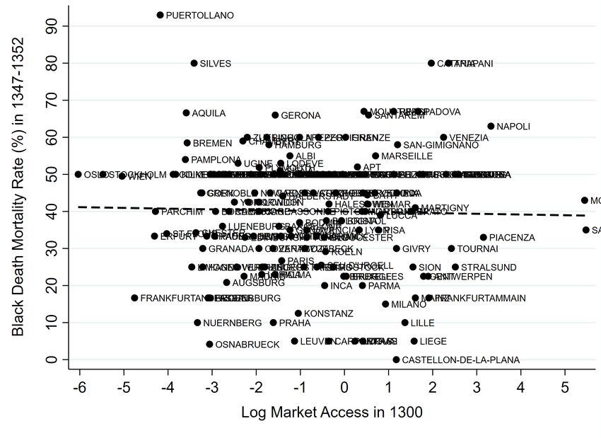
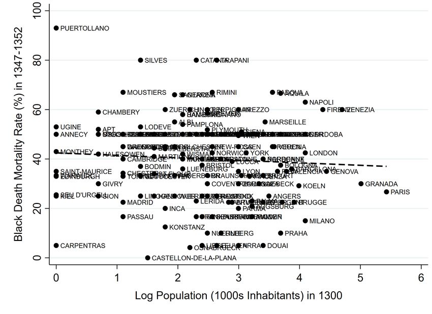
Figure 3(a) illustrates the lack of a relationship between mortality (1347-52)
and city population in 1300 (Y = 42.5*** - 1.01 X; Obs. = 165; R2 = 0.00) in
our sample of 165 cities. For the 88 cities with data on walled area we also
find no relationship with population density (Web Appx. Fig. A.4). Likewise,
Fig. 3(b) indicates no relationship between mortality and log market access in
1300 (Y = 40.0*** -0.20 X; Obs. = 124; R2 = 0.00). Note that random measurement
error in dependent variables (mortality) does not lead to bias. However, random
measurement error in market access produces a downward bias, and non-
classical measurement error is possible. Reassuringly, Web Appx. Table A.3 shows
no correlation when: (i) using a lower trade elasticities in the market access
calculation (2 or 1, instead of 3.8);7 (ii) using alternative measures of transport
costs or Euclidean distance, which has the advantage of not having to rely
7
We use a high sigma because trade costs were high and trade was limited then (relative to
today), much like in 19th century India for which sigma = 3.8 was estimated (Donaldson, 2018).12
on speeds related to plague diffusion itself;8 (iii) including the city itself;9 (iv)
including other (mostly Eastern) European cities not in our main sample of 16
countries; and (v) including cities of the Middle East and North Africa.10
Subsequent outbreaks of bubonic plague took place for two and a half
centuries following the Black Death. Epidemiologists and historians have long
noted the virulence, spread, and associated mortality of the Black Death differed
from the pattern associated with later outbreaks of bubonic plague (see Web
Appendix Section 5.). These plague recurrences were caused either by local
plague reservoirs or the reintroduction of the bacteria from Asia (Schmid et al.,
2015). Though on occasion later outbreaks could devastate a city, in general
mortality was significantly lower than in the initial pandemic (Aberth, 2010, 37).11
To summarize, on average, random factors must have compensated for non-
random factors, making Black Death mortality apparently locally exogenous.
3. The Black Death Shock and City Recovery
To estimate the short- and long-run effects of Black Death mortality on city
growth we estimate a series of city-level regressions based on (Hypothesis H2):
% Popi,t = ↵ + t Morti,1347 52 + ✏i,t (1)
where % Popi,t is the percentage population growth (%) in city i over period t-
1 to t, and Morti,1347 52 is the city-level cumulative mortality rate (%; 1347-52). We
weight observations by their population size in year t-1 to minimize issues arising
from smaller cities mechanically experiencing larger percentage changes.12
Col. (1) of Table 1 measures the short-run impact in 1300-1400. The
8
Boerner and Severgnini (2014) find that traveling by sea was 1.4 and 2.9 times faster than
traveling by river or road. We then assume that walking on a path was twice slower than traveling
by road (and thus 5.7 slower than traveling by sea). They also cite other estimates from Pryor
(1992) and McCormick (2001) that lead to a different combination: (3.8; 3.8; 7.7).
9
To avoid a zero trade cost, we use the travel cost between Paris and Saint-Denis, two localities
7 km away from each other (Saint-Denis is now part of Paris). Paris’ radius was smaller then.
However, to account for likely intracity congestion, we do not adjust down the travel cost.
10
We use the data of Bosker et al. (2013). Consequently, only 10,000+ cities are included.
11
Only the plague of 1629-30 in Italy came close to the Black Death’s virulence (Alfani, 2020).
12
Growth for a city of 1,000 in t-1 and 5,000 in t is 400%. Large cities rarely experience such
growth rates. While this is a standard issue when using percentage growth outcomes, we choose
this as our main specification because the interpretation of the coefficient is straightforward.13
coefficient, -0.87***, should be interpreted relative to the immediate effect in
1347-52, which is -1.00 by construction. The fact that the coefficient is not
significantly different from -1.00 suggests little recovery in the decades directly
following the onset of the Black Death. The effect is large: a one standard
deviation increase in mortality is associated with a 0.31 standard deviation
decrease in population growth. The effect in 1300-1500 is negative (-0.28,
col. (2)) but smaller in size compared to the effect in 1300-1400 and significantly
different from -1. Col. (3)-(5) examine the cumulative effect up to 1750. The
coefficient increases to 0.36, 0.47 and 0.85 by 1600, 1700 and 1750 respectively.
However, the magnitudes are small: A one standard deviation increase in
mortality is associated with between a 0.03 and 0.05 standard deviation increase
in population growth in columns (3)-(5) implying total recovery.
Parallel Trends. Col. (6)-(7) of Table 1 show that prior to 1300, there is no
difference in growth between cities most affected and those comparatively
unaffected by the plague. However, standard errors are not nil, so the pre-Black
Death effects are imprecisely estimated. The sample sizes show that many cities
also did not exist (i.e. were below 1,000 population) before 1300. Since col. (6)-
(7) examine the intensive margin of city growth, we show in col. (8)-(9) that the
likelihood of being above 1,000 by 1200 or 1300 is not correlated with mortality.
Correlates of Mortality. Table 2 shows that mortality rates were uncorrelated
with various city characteristics capturing physical geography (1), access to
markets and trade (2) or institutions (3). The only variables that have explanatory
power are proximity to rivers and latitude. However, the sign on proximity to
rivers is negative which is inconsistent with the claim that trade routes were
correlated with plague virulence. Other measures of transportation and trade
networks do not predict mortality. The coefficient on latitude reflects the fact that
the Black Death hit southern Europe first and was more virulent in the early years
of the epidemic. Finally, no effect is significant once all controls are included.13
13
The R2 in Col. (1) falls to 0.08 when we exclude latitude and temperature (correlation with
latitude of 0.77). If we re-run the specification in Col. (4) while dropping latitude and temperature,
the coefficients of the other controls remain insignificant and the R2 decreases to 0.18. It does not14
In row 2 of Table 3, we show the baseline results hold when we include all the
controls of Table 2 simultaneously. The effect in 1300-1400 is now less negative.
Indeed, we will show in Section 5. that city characteristics affected the recovery
of higher-mortality cities in 1353-1400 and beyond. Over-controlling might then
lead us to under-estimate the negative short-run effects.
Spatial Fixed Effects. In row 3 we include fixed effects corresponding to modern
country borders. As modern country borders differ from the political units of
the fourteenth century, in row 4 we assign a separate dummy variable to each of
the independent polities with at least 5 cities in our data set (Web Appx. Fig. A.5
shows state boundaries).14 Alternatively, we use fixed effects corresponding to
twelve 5x5 degree cells (row 5). The results that we obtain are qualitatively similar.
We then employ three instrumental variable strategies: IV1, IV2 and IV3. IV1
and IV3 rely on the date of first infection in the city, which is available for 124
cities.15 Also, since the IV strategies rely on the spatial diffusion of the Plague, we
cluster standard errors at the state (1300) level (N = 64) for these analyses.
IV1: Timing of Infection IV1 exploits the randomness in plague intensity
generated by the travel path of the disease. As discussed above, the Black Death
was most virulent initially, and over time virulence declined. We create a variable
for date of first infection for each city in our dataset. Fig. 2(a) plots mortality
rates against the date that the city was first infected (number of months since
October 1347). Cities infected later, indeed, had lower mortality. We therefore
use the number of months since October 1347 as an instrumental variable. We
add the controls of Table 2 (incl. longitude and latitude) and include the squares
and cubes of longitude and latitude. The estimates we obtain are similar to our
OLS estimates (row 6 of Table 3; -1.07** and 0.05; IV-F stat = 11.8).
IV2: Proximity to Messina IV2 is based on distance to the point of first infection,
Messina. The logic behind IV2 is similar to IV1: as the virus was more virulent
decrease to 0 because some of the remaining variables are still correlated with latitude.
14
The sheer number of states (44; source: Nussli (2011)) raises a potential problem as many had
only a single major city. Hence we use fixed effects for 7 larger states with at least 5 cities.
15
See Web Appx. Table A.4 for the full first-stage regressions for IV1, IV2 and IV3.15
initially, locations that were connected to Messina were more likely to be infected
earlier and hence more likely to suffer high rates of mortality.
We use as an IV the Euclidean distance to Messina, conditional on average
Euclidean distance to all cities in Western and Eastern Europe and the Middle
East and North Africa (using their 1300 population as weights). Controlling
for average distance to all cities captures the fact that some cities were
better connected overall. Hence, we exploit the fact that it was the specific
connectedness to Messina, and not connectedness overall, that mattered for
mortality. In addition, since we use Euclidean distances, our IV is not built using
the (possibly endogenous) speeds of plague transmission. We add the same
controls as for IV1, including the controls for the various means of transportation.
Controlling for longitude and latitude (and allowing them to have non-linear
effects) is important because it captures any South vs. North and East vs. West
effects. We report the IV estimates in row 7. The short-run coefficient (-1.20**)
is similar to our OLS estimate (IV F-stat = 22.6). The long-run effect is negative
(-0.68), but half the size of the short-run effect and not significant.16
IV3: Month of First Infection IV3 uses the variation in mortality generated
by differences in the month of first infection within a single year. For 124
cities for which we have data on the onset of the plague, Fig. 2(b) shows the
relationship between mortality and the month of peak infection in the city
(= month of onset + 3.5 months). The plague was more virulent when peak
mortality occurred during summer (6-8) (the quadratic fit omits January, which
has abnormally high mortality due to October being the month of onset of the
plague in Europe). We report results using IV3, dummies for the month of peak
infection, while adding the controls used for IV1 and dummies for the year of
first infection to control for the fact that cities infected in earlier years had higher
16
For this IV, we use cities above 1,000 in Europe and cities above 10,000 in the Middle East and
North Africa (estimates not available below). What could matter for trade to influence mortality
could be proximity to large cities only, or proximity to many cities. We take an intermediary
approach and use as weights log population in 1300, thus giving less weight to the largest cities.
Results hold if we: (i) control for average distance to all cities above 10,000 only; and (ii) use as
weights unlogged population – giving more weight to large cities – or no weights – making a high
spatial density of cities important – when computing the distance to all cities (not shown).16
mortality. We obtain similar results (row 8; -0.93*** and -0.23; IV-F stat = 6.0).17
Lastly, results hold when using the three IVs simultaneously (row 9).
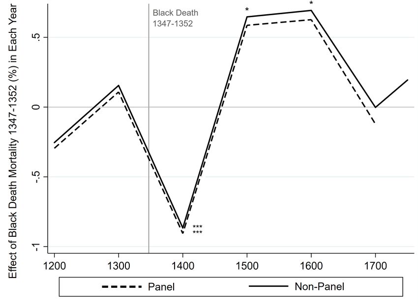
Panel Analysis. To do this we restrict the sample to the 165 cities that are in our
dataset in 1300 and for which we know Black Death mortality rates. We focus our
analysis on the years 1100, 1200, 1300, 1400, 1500, 1600, 1700 and 1750. We then
estimate the following regression equation:
% Popi,t 1!t =↵+ t Morti,1347 52 + i + ✓t + ✏i,t (2)
where the dependent variable is the percentage change in population between
t-1 and t (1100 is dropped), where city (i ) and year (✓t ) fixed effects are included,
and where the variables of interest are mortality in 1347-52 interacted with the
year dummies ( t shows the effect in each year relative to the omitted year 1750).
We use as weights population in t-1 and cluster standard errors at the city level.
Figure 4 shows the interacted effects (“Panel”) and the corresponding effects
when running the cross-sectional regression for each year one by one (“Non-
Panel”). The negative effects in 1300-1400 (“1400”; about -0.9***) are offset by
positive effects in 1400-1500 (“1500”) and 1500-1600 (“1600”) (coefficients shown
in Web Appx. Table A.5), implying city effects do not have important effects.
Robustness. These results are robust to additional concerns about causality,
specification, data measurement, sample size, and sampling.
The Black Death was attributed to the “vengeance of God” or the “‘conjunc-
tion of certain stars and planets” (Horrox, ed, 1994, 48-49). Thus, there was little
variation in a city’s ability to deal with it. Historians report that some cities had
either natural baths (Bath, Nuremberg) or tried to take action in response to the
plague (Milan, Venice). Results hold when we drop these (Web Appx. Table A.6).
Neither the medical profession nor authorities could respond. Medical knowl-
edge was rudimentary: Boccaccio (2005, 1371) wrote that “all the advice of physi-
17
If we study the relationship between mortality and the month of peak infection in the city for
warmer regions vs. colder regions, we find even lower mortality rates in the winter in cities located
in colder regions (Web Appx. Fig. A.6). Using as an IV dummies for the month of peak infection
interacted with the log of a city location’s average temperature, the IV-F stat increases to 7.2. The
coefficients remain very similar to the coefficients for IV3 (row 15 of Web Appx. Table A.6).17
cians and all the power of medicine were profitless and unavailing”. Individuals,
regardless of wealth, could not protect themselves. Prevention measures were
nonexistent: the practice of quarantine was not employed until 1377.18 Other
practices such as separating the sick and burning the homes of the infected were
also introduced after the Black Death period (1347-1352).
Bubonic plague reoccurred following the Black Death. This could be
a source of bias if subsequent outbreaks were correlated with the initial
pandemic. We use data from Biraben (1975) and show results hold if we
control for plague recurrences (see Web Appx. Table A.6 for details).19 The
Black Death initially reduced the intensity of conflict (see Sumpton (1999)).
However, warfare ultimately intensified and, according to some accounts, led
to urbanization (Voigtländer and Voth, 2013a). We show results hold if we
control for contemporaneous or past battles (Web Appx. Table A.6), or control
for proximity to a battle of the Hundred Years’ War prior to the onset of the Black
Death. Results also hold if we control for the number of famines experienced
by the city’s region or country, or the possible magnitude of the Great Famine of
1315-1317 (same table). Finally, Jedwab et al. (2019) show that higher-mortality
cities persecuted Jewish communities less. Results nonetheless hold if we control
for persecutions or drop any city with a persecution (Ibid.).
Similarly, our findings are robust when we: (i) consider other specifications,
for example control for past population trends or study absolute changes
in population; (ii) cluster standard errors differently; (iii) take into account
measurement error arising from the coding of mortality rates; (iv) focus on cities
that are either in the bottom 10% of least affected cities or in the top 10% of most
affected cities, since measurement errors in mortality rates are more likely when
comparing cities with similar rates; (v) use alternative population estimates; and
(vi) address concerns regarding the external validity of our results, for example
increase sample size by using imputed mortality rates for cities outside our main
18
The term quarantine was indeed first used in Ragusa in Croatia in 1377 (Gensini et al., 2004).
19
Subsequent plagues were not correlated with mortality (Web Appx. Table A.7). Later
recurrences also had a different epidemiology to the initial outbreak (Web Appx. Section 5.).18
sample (Web Appx. Table A.8). Lastly, we drop cities located within France,
Germany, Italy, the United Kingdom or Spain (Web Appx. Table A.9).
Overall, the various regressions return similar estimates to those obtained
using the baseline OLS cross-sectional regressions. This reassures us that plague
mortality had a strong locally exogenous component (H1). In the rest of the
analysis, and for the sake of simplicity, we employ the baseline OLS specification.
4. The Black Death as a Regional Shock
So far, we have only discussed the effects of own city mortality on city growth.
However, we need to quantify spillover and general equilibrium effects in order
to test the recovery hypothesis for urban systems, not just individual cities.
These effects are interesting in their own right because the population declines
associated with the Black Death reduced market potential across Europe. In this
sense, it was a massive trade shock that allows us to investigate Hypothesis H3.
Table 4 studies the effects of a city’s own mortality and the spillover effects
from mortality in other cities. Col. (1) reproduces the city-level results. In col. (2)-
(3), we estimate the effects of population-weighted average mortality at the state
level on the percentage change in urban population at the state level.20 Col. (2)
shows the effects for cities that existed in 1300. Our baseline estimate of the
short-run impact of the Plague suggests that a city with a 10% mortality rate was
only 8.7% smaller fifty years later. In contrast, col. (2) suggests that if an entire
region experienced average mortality of 10%, then a city with a 10% mortality
rate would have shrunk by 11.5% by 1400. Col. (3) examines the effects on all
cities that are in the dataset in 1400 (including cities not in the dataset in 1300).
The effects are larger than before (-1.47**) implying that in high-mortality areas,
fewer new cities emerged, a result we explore in more detail below.
Similarly, when we look at the long-run effects in Panel B, we find that unlike
the impact of a city’s own mortality rate, the effect of aggregate mortality is
negative (though the standard errors are very large, implying heterogeneity).
20
For this analysis, we include all 1,801 towns, and use spatially extrapolated mortality rates for
towns without mortality data and population = 500 inhabitants for towns with population below
1,000. We lose 20 states and 1 country (Luxembourg) without any urban population in 1300.19
This is consistent with the Black Death shock having broader, negative,
disintermediation effects on local economies (Broadberry et al., 2015, Ch. X).
In columns (4) and (5), we define “indirect mortality” as the average mortality
rate of the cities of the same state and of the closest 10% of cities, respectively.
Note that cities that experienced high mortality did not always experience high
indirect mortality (the correlation between the two measures is less than 0.5 in
both cases). We again find suggestive evidence that indirect mortality had a
negative impact on population between 1300-1400 (the coefficient is large and
negative but imprecisely estimated). The combined effects of mortality and
indirect mortality are about -1.00, and significant (not shown).21
We also explore how the Black Death shaped the emergence of new cities
and the transition of smaller urban settlements into cities. Recall that our
dataset contains 1,801 cities but that 1,335 of these cities are not present in
the year 1300. These cities can be thought of as the universe of potential city
locations. In column (6), we look at the effect of Black Death mortality rate on
whether a city enters ours dataset in 1400. To do this we use our extrapolated
mortality rate estimates. We find that cities were less likely to emerge when their
extrapolated mortality rate was high. Likewise, we regress the log population
of these 1,335 cities (using 500 for cities below 1,000) on mortality and find
that fewer locations became urbanized in high-mortality areas (column (7)).
Consistent with previous results, we find that these negative effects of the Black
Death disappeared by 1600 (Panel B). This suggests that in the long-run, the Black
Death did not delay the transition of villages into cities.
Finally, we investigate how the Black Death might have impacted rural areas.
In Web Appx. Section 6., we use historical deforestation data to show how, in
high-mortality regions, rural areas recovered slower than urban areas. Since
21
Results hold if indirect mortality is constructed using cities of the same modern country
or using all 1,801 cities but relying on the change in market potential 1300-1353 (not shown).
To construct market potential in 1353, we use the predicted population of the other towns in
1353 (= pop1300 *(100-mort.)). Since mortality is only available for 274 cities, we use spatially
extrapolated mortality rates for 1,527 cities. For each of the 165 observations, the mortality rates
of the other towns are constructed excluding the mortality rate of the observation itself.20
land use recovered slowly in the aggregate, it must be that marginal rural areas
suffered relatively greater population losses following the Black Death. Data on
the desertion of villages in England confirm this result, suggesting that many
of the individuals who came to repopulate high-mortality cities and regions
came from more rural areas in lower-mortality regions. In the Web Appendix
we explain that this was probably driven by wages rising relatively more in
high-mortality urban areas in the aftermath of the shock. Lastly, we further
support this explanation using localized data on fertility regimes, confirming that
migration, not fertility, was behind city population recovery.
5. Heterogeneity in City Recovery
In a Malthusian economy a pandemic might have no long-term spatial effects
on average. Nonetheless, there could be still permutations among cities as some
large cities become relatively smaller, and small cities, relatively larger. These
permutations may in turn be affected by how mortality and the pre-pandemic
characteristics of these cities interact (Hypothesis H4).
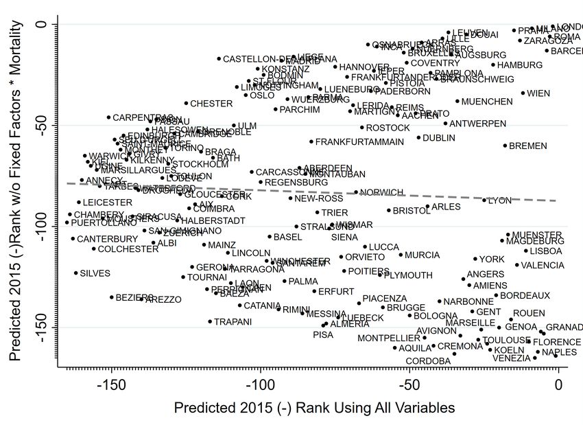
Permutations. Historical evidence suggests there was heterogeneity across cities
in the response to the Black Death.22 For our sample of 165 cities, we regress the
rank of each city in 1600 on its rank in 1300 and find a slope of 0.86***. Hence,
large cities tended to remain large and small cities tended to remain small.
However, the R2 is 0.56, suggesting that aggregate recovery hides permutations.
Figure 5(a) illustrates this, with many cities far from the forty-five degree line.
We test whether these permutations were associated with some of the
characteristics considered in Table 2. We modify Eq. 1 by interacting mortality
(Morti,1347 52 ) with selected city characteristics (Chari ) while controlling for the
characteristics themselves and mortality:
% Popi,t = ↵ + t Morti,1347 52 + Morti,1347 52 ⇤ Chari ✓ + Chari ⇠ + ✏i,t (3)
Throughout, we focus on our main sample of 165 cities, for the period 1300-2015.
For two cities experiencing the same mortality shock (e.g., 50%), the vector ✓
22
Campbell (2016, 365) notes that “towns competed with each other in an urban survival of the
fittest.” See Web Appx. Section 7. for a lengthier discussion of the permutations in the data.21
captures the differential recovery effects of each characteristic.
Interpretation of ✓. If labor becomes scarce in both cities but one city has impor-
tant local factors complementary to labor, net wages should disproportionately
increase there, attracting people. The city’s population then recovers relative to
lower-mortality cities. With high migration costs (including information costs),
relative recovery will be slow enough that the negative effect of mortality may
not have been fully offset by 1400 or even 1500. In the longer run, locations
recovering faster thanks to advantageous characteristics may also gain a long-
run productivity advantage and grow relatively faster. Thus, ✓ will be significant
immediately after the shock and its magnitude may also increase in later periods.
An alternative scenario is when one highly impacted city has a local factor
that is not valuable immediately after the Black Death shock (e.g., given the state
of technology). Initially, the city will not recover faster than another equally
impacted city. However, once the factor becomes valuable (which may occur a
few centuries later), this helps the city escape the low-population equilibrium in
which the Black Death shock put it. ✓ would then be small for some time before
increasing in magnitude and possibly turning significant.
Factor Selection. With 165 cities, we cannot add all 27 variables of Table 2 and
their interactions with mortality. Instead, we select those that proxy for: (i)
land quality: the three agricultural suitability measures (cereal, potato, pastoral);
and (ii) access to markets and trade: coastal and river dummies, Roman road
or medieval land route intersections, and the Hanseatic League dummy. Coast
and rivers lowered transportation costs. Roman roads remained the basis of the
road network in the medieval era (Dalgaard et al., 2018b). Medieval trade routes
reflected long-established trading linkages. We include factors proxying for (iii)
agglomeration effects as the log of the estimated population of the city in 1353
(= pop.1300 x (100-mort.)/100). Finally, we proxy for (iv) institutions using three
dummies for whether the city was part of a monarchy, was a state capital, and
whether it had a representative body (c. 1300).23
23
Lasso regressions cannot be implemented because current Lasso programs do not allow for
regression weights (we use as weights city population in 1300). In addition, one major reason to22
Identification. Table 5 shows the 11 interacted effects, for 1300-1750 (col. (1)-(5))
and 1300-2015 (col. (6)). The 11 interacted effects are simultaneously included in
the model and show the recovery effect associated with each factor conditional
on the recovery effect associated with each other factor. With 165 observations
and 23 variables, this makes our test particularly stringent. Note that we show
the interacted effects for the period 1300-1400 because cities started recovering
in 1353-1400. We thus use 1300 as the start year instead of 1353 because we do
not know the true population of each city in 1353.24
We do not use panel or IV regressions for this analysis as we have
demonstrated above that these methods return results that are similar to OLS.
We thus rely on the baseline OLS cross-sectional regression for its simplicity
and transparency. However, since we cannot be entirely sure that mortality was
indeed exogenous, the results in this section should be taken with caution.25 For
the sake of conciseness, and since what only matters are the interactions with
mortality, we also do not report the independent effect of each factor.
Land Quality. The coefficient on mortality*cereal suitability is positive (but
not significant) after 1400 (col. (2)). However, the implied economic impact is
meaningful since the beta coefficient (henceforth, “beta”) reaches 0.47 by 1600
and remains high thereafter (0.17 in 2015). The 1600 coefficient of 0.47 is half of
the standardized effect for mortality. In other words, places with 1 SD higher
cereal suitability recovered twice as fast as cities with poor cereal suitability
experiencing the same mortality rate. Potato suitability may have also helped
highly impacted cities escape their post-plague low-population equilibrium from
the 17th century onwards (col. (4)). Nunn and Qian (2011) show that countries
that were more suitable for potato cultivation urbanized faster after potato
use Lasso techniques is to make a model sparser in order to reduce muticollinearity. However,
the 11 factors are only weakly correlated (mean correlation for the 11 x 10 ÷ 2 = 55 combinations
⇡ 0.15). Lasso regressions also cannot tell us which other factors from Table 2 should be added.
24
The Bairoch data set stops in 1850. Cities have also grown dramatically since 1850, becoming
multi-city agglomerations. We read the webpage of each city in Wikipedia and selected the 2015
population of the city itself rather than the population of the agglomeration. Results, however,
hold if we use the agglomeration estimate or the mean of the two estimates (not shown).
25
We have 23 variables and 165 cities. Adding interactions of each factor with instruments
would leave us with no variation, and mechanically creates multiple weak instruments.23
cultivation diffused in Europe (the non-effects in col. (1)-(3) are reassuring).26
In high-mortality areas suitable for pastoral farming we find a negative effect
in 1500-1600 (col. (3)) and no effects before (col. (1)-(2)). The effect in 1500-
1600 is strong (beta = -0.64) and becomes weaker over time (beta = -0.25 in
2015). We believe this is caused by higher wages due to labor shortages that
created incentives for landlords to specialize in pastoral agriculture, thus further
reducing the need for labor (Voigtländer and Voth, 2013a, p. 2255).27 As seen, the
effect only became significant in the 16th century. Indeed, pastoral farming as
a solution to labor scarcity and rising wages did not arise immediately or across
Europe (Jedwab et al., 2021). This effect diminishes after 1750.28
Agglomeration Economies. The literature (e.g., Duranton and Puga, 2004) dis-
tinguishes economies of scale – in production, market places, and consumption
– and agglomeration economies strictly defined, according to which a larger pop-
ulation increases productivity and wages, which should cause in-migration. In
row 8 of Table 5 we interact estimated city population in the immediate aftermath
of the Black Death with mortality to investigate if the population shock reduced
agglomeration economies, thereby slowing recovery. We find no economically or
statistically significant effects, suggesting that agglomeration economies did not
play a major role in city growth at this time.
Access to Markets and Trade. The interacted effect for coastal proximity is one
of the only two significant coefficients in 1300-1400 (col. (1)) along with the
interacted effect for the Hanseatic league. While the coefficient of mortality is
-3.9, the coefficient of mortality*coastal proximity is 1.2. Thus, relative to non-
coastal cities, coastal cities recovered almost 33% faster by 1400. In 1500, the
26
The country-level effects of Nunn and Qian (2011) appear in 1750, whereas our interacted
effects appear in 1700 because we focus on the local level. Indeed, the local cultivation of the
potato started in the late 16th century and became widespread in the late 17th century (Nunn
and Qian, 2011, p.601-603). Our effect is still large, and significant, in 2015 (beta = 1.06).
27
This effect is consistent with contemporary accounts. E.g. In 1516 Sir Thomas Moore wrote
in Utopia, “Your sheep. . . that commonly are so meek and so little, now, as I hear, they have
become so greedy and fierce that they devour men themselves.”
28
This may reflect the rise of labor-intensive proto-industry in rural areas, in particular textile
production, which was associated with more rapid population growth (Mendels, 1972; Pfister,
1989). Wool was the most common textile used in making clothing.You can also read