Optical phantoms with variable properties and geometries for diffuse and fluorescence optical spectroscopy
←
→
Page content transcription
If your browser does not render page correctly, please read the page content below
Optical phantoms with variable
                 properties and geometries for diffuse
                 and fluorescence optical spectroscopy

                 Barbara Leh
                 Rainer Siebert
                 Hussein Hamzeh
                 Laurent Menard
                 Marie-Alix Duval
                 Yves Charon
                 Darine Abi Haidar

Downloaded From: https://www.spiedigitallibrary.org/journals/Journal-of-Biomedical-Optics on 19 Jun 2022
Terms of Use: https://www.spiedigitallibrary.org/terms-of-use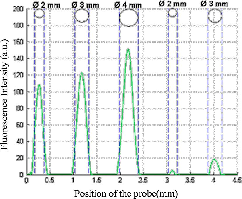
Journal of Biomedical Optics 17(10), 108001 (October 2012)

                Optical phantoms with variable properties and geometries
                for diffuse and fluorescence optical spectroscopy
                Barbara Leh,a Rainer Siebert,a Hussein Hamzeh,a Laurent Menard,a,b Marie-Alix Duval,a Yves Charon,a,b and Darine Abi
                Haidara,b
                a
                    Laboratoire IMNC, UMR 8165, F-91405 Orsay Cedex, France
                b
                    Université Paris 7, F-75012 Paris, France

                              Abstract. Growing interest in optical instruments for biomedical applications has increased the use of optically
                              calibrated phantoms. Often associated with tissue modeling, phantoms allow the characterization of optical
                              devices for clinical purposes. Fluorescent gel phantoms have been developed, mimicking optical properties of
                              healthy and tumorous brain tissues. Specific geometries of dedicated molds offer multiple-layer phantoms with
                              variable thicknesses and monolayer phantoms with cylindrical inclusions at various depths and diameters. Organic
                              chromophores are added to allow fluorescence spectroscopy. These phantoms are designed to be used with
                              405 nm as the excitation wavelength. This wavelength is then adapted to excite large endogenous molecules.
                              The benefits of these phantoms in understanding fluorescence tissue analysis are then demonstrated. In particular,
                              detectability aspects as a function of geometrical and optical parameters are presented and discussed. © 2012 Society of
                              Photo-Optical Instrumentation Engineers (SPIE). [DOI: 10.1117/1.JBO.17.10.108001]

                              Keywords: optical properties; spectroscopy, tissue diagnostic; turbid media, fluorescence.
                              Paper 12245 received Apr. 21, 2012; revised manuscript received Aug. 24, 2012; accepted for publication Aug. 27, 2012; published
                              online Oct. 4, 2012.

                1      Introduction                                                                phantoms, microspheres like polystyrene beads can be used
                In biomedical applications, the interest in novel optical                          instead.5,6 Several types of microsphere compositions covering
                approaches has grown and consequently so has the use of opti-                      the anisotropy scattering range of tissues and different diameters
                cally calibrated phantoms. A phantom is a tool that provides                       are available as SiO2-304 nm (anisotropy coefficient g ¼ 0.82
                known or determined parameters that can be used to characterize                    and scattering cross-section σ sca-cm2 ¼ 2.73 × 10⁻¹² ), SiO2-
                and/or calibrate experimental devices and to understand the bio-                   585 nm (g ¼ 0.94 and σ sca-cm2 ¼ 4.21 × 10⁻¹¹ ) and Melamine
                logical data. Optical phantoms are widely used for developing,                     MF 410 (g ¼ 0.87 and σ sca-cm2 ¼ 1.91 × 10⁻¹⁹ ). A commonly
                testing and optimizing optical instrumentation for fluorescence,                   used absorber is ink.7,8 Sometimes fluorescence characteristics
                diffuse reflectance and Raman spectroscopy.1,2 Optical phantoms                    are also required.3,7–9 A phantom can include several types of
                are important to link experimental results to theoretical models.                  fluorophores that might be either organic fluorophores, such as
                    Depending on their use, various optical phantoms exist in                      Rhodamine 6G6,8 or Protoporphyrin IX,7 or fluorescent particles,
                varying consistencies, shapes, employed components, optical                        such as coloured resins,3 quantum dots9 or endogenous fluoro-
                ranges, etc.                                                                       phores.10 Due to their hydrophobic property, solid phantoms can-
                    When defining a new phantom, the first step is to clearly                      not contain organic or biological fluorophores.
                identify its desired functionalities. Among these functionalities                      In this paper, new gelatin phantoms are presented that mimic
                is the stability over time to get optical references that allow cali-              brain tissue properties. These phantoms should help to define
                bration of optical systems or comparison of different setups.                      and optimize a new prototype fiber optic instrument. This instru-
                Most of the time, these stable phantoms are solid and made                         ment is dedicated for surgical treatment of brain tumors by dis-
                out of polymers3,4 and do not typically model the anatomic                         criminating healthy from tumorous tissues through endogenous
                shapes and chemical composition of tissues. Liquid or gelatine                     fluorescent measurements. Two geometries are used-bilayer
                phantoms can be an alternative when long-term stability is not                     phantoms and phantoms with inclusions. The first models
                required. To imitate biological tissues, different layers are often                tumorous and healthy tissue layers, whereas the latter mimics
                required, such as mimicking tumors in healthy tissues. In the                      cylindrical tumors in a healthy environment.
                case of multi-layer phantoms, several options are possible,                            It is our intention to use the phantoms to simulate the follow-
                such as successive gel layers5 or one solid layer with a liquid                    ing situation: a cancerous layer of various thicknesses is placed
                layer above.6                                                                      in front of a noncancerous layer or vice versa. In the first case, it
                    Other characteristics of phantoms are their geometry and opti-                 will allow for identification of the minimum thickness of can-
                cal properties, the latter being mainly defined through the refrac-                cerous tissue necessary to be detectable with the probe. In the
                tive index and scattering and absorption coefficients. The most                    latter case the maximum layer thickness of noncancerous tissue
                common tissue-like phantom scatterers are intralipids,7,8 used                     would be estimated to still allow for detecting the cancerous
                generally in liquid phantoms. In the case of gelatine or solid                     layer behind. In this first study, different fluorophores are
                                                                                                   used for the two types of tissues. This is the easiest way to

                Address all correspondence to: Darine Abi Haidar, Laboratoire IMNC, UMR
                8165, F-91405 Orsay Cedex, France. E-mail: abihaidar@imnc.in2p3.fr                 0091-3286/2012/$25.00 © 2012 SPIE

                Journal of Biomedical Optics                                               108001-1                                         October 2012   •   Vol. 17(10)

Downloaded From: https://www.spiedigitallibrary.org/journals/Journal-of-Biomedical-Optics on 19 Jun 2022
Terms of Use: https://www.spiedigitallibrary.org/terms-of-use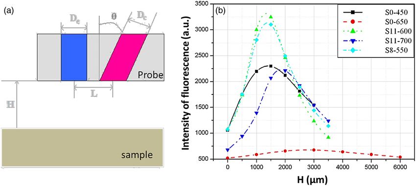
Leh et al.: Optical phantoms with variable properties and geometries for diffuse and fluorescence : : :

                know where the detected photon originates and to get a first-                      degree and L in micrometer. As shown in Fig 1(b), the S11-600
                order estimate of detectable configurations. In a future extension                 probe was identified as collecting the highest fluorescence inten-
                of the study, different fluorophores will be used with different                   sity and so was chosen for the present work. The best fluores-
                concentrations in each layer to analyze the impact on the detect-                  cence collection is obtained with an around 11 deg tilted fiber,
                ability of cancerous tissue.                                                       the fiber distance being around 600 μm. The optimal distance
                    The optical parameters of brain tissue were taken from litera-                 between the tissue and the probe, allowing for detection of
                ture.11,12 Gelatine phantoms are well suited to reach these dif-                   the maximal intensity, is 1.5 mm and the spatial resolution of
                ferent geometries. In addition, organic chromophores that                          this probe is about 500 μm measured by using a test target
                emit in the range of endogenous fluorophores were chosen.13                        (R3LS1P, Thorlabs, France). The collected light is filtered by
                We also took into account the wavelength dependence of                             a high-pass filter (M54-650, Edmund Optics, Barrington NJ,
                these phantoms for fluorescence study. Our phantoms have                           USA) before being analyzed by a spectrometer (QE6500,
                the specificity to be excited at 405 nm, an interesting excitation                 Ocean Optics, Dunedin FL). Figure 2 shows a diagram of the
                wavelength for endogenous fluorophores, much like nicotina-                        experimental device. The setup was similar to the one used in
                mide adenine dinucleotide (NADH), flavins, lipopigments, por-                      our previous work.15
                phyrins and chlorins.14 Most of the time optical commercial
                phantoms are calibrated to be excited at wavelengths longer                        2.2     Phantoms—Optical Properties
                than 450 nm. For an endogenous fluorescence study of cerebral
                tissues, 405 nm is an interesting choice of excitation wave-                       In the present work, the purpose of the phantoms is to charac-
                length. Our phantoms are also used to validate physical models                     terize a probe for auto-fluorescence brain tissue measurements.
                and a Monte Carlo simulation.                                                      Thus, the different components of the phantoms should offer
                                                                                                   brain tissue optical parameters.
                2     Materials and Methods
                                                                                                   2.2.1    Refractive index
                2.1     Experimental Setup
                                                                                                   Gelatine from porcine skin (A-type, G1890, Sigma-Aldrich,
                The light source is a 405-nm-pulsed-laser (PicoQuant, Berlin,                      Saint Quentin Fallavier, France) was used. It is well suited to
                Germany); its frequency is up to 40 MHz with a pulse width                         our phantoms because it produces very little fluorescence
                of less than 100 ps and a maximum power of 1 mW. A                                 when excited at 405 nm. For all gels, a mixture of water and
                home-made 2-fiber-probe has been used [Fig 1(a)]. The fibers                       10% gelatine powder was employed. Measurements of solid
                used are step index multimode Si-fibers. More details of this                      gelatine made by our team,16 basing on Snell’s law, yielded a
                probe are described in Ref. 15. The excitation and the fluores-                    refractive index of 1.40  0.01. This index corresponds to the
                cence collection fibers have a 200 and a 365 μm core-diameter,                     refraction parameter of biological tissues.17
                respectively. Several probe configurations were previously
                tested by our group15 for varied fiber distance L and inclination                  2.2.2    Absorption
                θ of the collection fiber relative to the excitation fiber (the dis-
                tance of the probe relative to the phantom/tissue was also taken                   India ink diluted in water (no. 17, Pelikan, Hannover, Germany)
                into account) to estimate the best fluorescence collection effi-                   was used. Light transmission measurements have been made for
                ciency. This was done through various ways: Geometrical exci-                      several ink concentrations to determine the absorption coeffi-
                tation/collection cone recovery of both fibers, measurements and                   cient μa . The samples were placed in quartz cuvettes and mea-
                simulations. The denomination of the fiber is Sθ-L, where θ is in                  sured with an UVICON 923 spectrometer (Bio-Tek Kontron

                Fig. 1 (a) Probe configuration, excitation fiber (De) and collection fiber (Dc). (b) Influence of the distance between probe and specimen on the collected
                fluorescence intensity.

                Journal of Biomedical Optics                                               108001-2                                         October 2012    •   Vol. 17(10)

Downloaded From: https://www.spiedigitallibrary.org/journals/Journal-of-Biomedical-Optics on 19 Jun 2022
Terms of Use: https://www.spiedigitallibrary.org/terms-of-use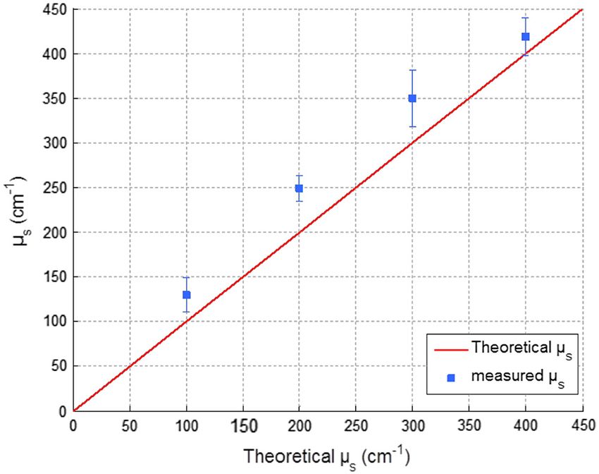
Leh et al.: Optical phantoms with variable properties and geometries for diffuse and fluorescence : : :

                                                                                                   program)15,19 for scattering spheres, knowing their diameter as
                                                                                                   well as their refractive index.
                                                                                                       From the literature in Refs. 11 and 12, we know that brain
                                                                                                   tissue μs is in the range from 100 to 400 cm−1 and the aniso-
                                                                                                   tropy varies from 0.75 to 0.95. MF-410 allows for obtaining the
                                                                                                   scattering coefficient in the interval of cerebral tissues. For a
                                                                                                   concentration of 100 mg∕ml and a density of 1.5 g:cm−3 and
                                                                                                   using a computed Mie theories (Fd Mie program) σ s was cal-
                                                                                                   culated to be 1.91.10−9 cm2 and g ¼ 0.87 using a 405-nm exci-
                                                                                                   tation wavelength.
                Fig. 2 Experimental device for fluorescence intensities measurements.

                Instrument, Milan, Italy). Transmission through a reference                        2.2.4   Optical properties measurements
                (water placed in the same cuvette) was also measured. The                          A single integrating sphere (IS200 Thorlabs) was used to mea-
                absorption coefficient is linear with the ink concentration                        sure reflection and transmission of 1-mm-thick phantom sam-
                (vol./vol.) Cink . A linear fit provided the calibration equation                  ples. Another device with diaphragms allows the
                that was used to obtain the defined μa . The absorption coeffi-                    measurement of the collimated transmission of the same sample.
                cient of gel and spheres was measured and it is equal to 2 cm−1 .                  The samples do not contain any fluorophore. The measured
                This absorption coefficient was taken into account when we cal-                    quantities are analyzed with the program inverse adding-dou-
                culate the concentration of ink for a wanted absorption coeffi-                    bling (IAD) (available at Ref. 19) to retrieve the optical coeffi-
                cient of our phantom. By this μa total ¼ μa ink þ μa gelþsphere .                  cients g, μa and μs . The anisotropy of scattering is found to be
                    In order to correspond to optical absorption coefficients for                  0.85  0.01, close to the expected value of 0.87. The measured
                brain tissues in literature,11,12 the absorption coefficient was var-              absorption coefficients also correspond to the expected ones if
                ied from 3 to 18 cm−1 . Note that after measurements the absorp-                   an offset of þ2 cm−1 is applied; this might be due to the gelatine
                tion due to the fluorophores was not taken into account: μa from                   and micro-particles absorption. The scattering coefficient is also
                the fluorophores was always less than 0.15 cm−1 and thus neg-                      overestimated by less than 10% compared to the expected value,
                ligible compared to the used ink absorption coefficients.                          which is considered acceptable. In conclusion, the phantoms we
                    Compared measurements between two sets of diluted ink in                       built were validated.
                water were made. One set (A) was diluted less than 24 h ago and
                the other one (B) was aged for about three months. The absorp-
                tion coefficient differed by around 15%, with the recent dilution                  2.2.5   Fluorescence
                seemingly more absorbent. Therefore to be completely sure that                     Either Rhodamine B (RhB) (Sigma Aldrich Fluka, Saint-Quen-
                ink dilutions are correct, we choose to always prepare the ink                     tin Fallavier, France) or Fluorescein (FITC) acide libre, (Sigma
                dilutions less than 48 h before casting the phantoms.                              Aldrich Fluka, Saint-Quentin Fallavier, France), each diluted in
                                                                                                   water, are also added to provide fluorescence in the phantom.
                                                                                                   Even if it is far off their absorption maximum, both absorb
                2.2.3    Scattering
                                                                                                   light at 405 nm. Moreover, RhB emits light at around
                Microspheres (micro-particles GmbH, Berlin, Germany) have                          580 nm, similar to Lipopigments, and FITC emission is around
                been used for finding the scattering properties of phantoms.                       515 nm, right in the Flavin range. A typical fluorophore concen-
                For our manipulation we used microspheres of Melamine MF                           tration used for our phantoms is 10−5 M. The absorption spectra
                delivered in 10% solution with these manufactured data                             of these molecules were measured by an absorption spectro-
                (410 nm of diameter, with a density of 1.51 g∕cm3 for each sphere,                 meter (UVICON 932, Bio-Tek, Kontron Instrument, Milan,
                the refractive index is 1.68) dispersed homogeneously in water. By                 Italy). The values of absorption coefficients of FITC and
                varying the concentration of spheres, we made suspensions with                     RhB at a 405-nm excitation wavelength, for a concentration
                the desired scattering properties. The dependence of the scattering                of 10−5 M are 0.13 and 0.15 cm−1 , respectively. These are
                cross-section σ sca and the anisotropy g on the wavelength accord-                 very weak compared with absorption coefficients of cerebral tis-
                ing to the parameters of spheres is established thanks to the Mie                  sues. Thus it is not necessary to make an additional correction to
                theory. They were computed using Mie theory (FdMie program,                        the definition of the ink concentration of the phantoms.
                based on Refs. 18 to 22). For a low concentration of scatterers
                (independent scattering approximation), the power scattered by                     2.2.6   Phantom fabrication protocol
                the unit volume is obtained simply by adding the power scattered
                by each particle. For independent scatterers, we can assume that                   Corresponding to the desired optical parameters, the concentra-
                the phantom-scattering coefficient is a linear function of the                     tions of each phantom component are calculated according to
                microsphere concentration, calculated using Eq. (1), where ρ is                    the above-mentioned methods. Water and ink are mixed before
                the density.21,23–26 We can use this approximation because the den-                the gelatine powder is added. This mixture is then heated in a
                sity ρ of our samples is lower than 0.01 (i.e., the volume occupied                90°C hot water bath. While the powder dissolves, the solution is
                by scattering particles is less than 1% of the total volume).27                    gently agitated to avoid air bubbles. Finally, fluorophores and
                                                                                                   scatterers are added and the mixture is placed in an ultrasound
                                              μs ¼ ρ · σ sca :                          (1)        bath for a few minutes to obtain a homogeneous solution. While
                                                                                                   still liquid, the gel is poured into a mold, which is subsequently
                   It is defined that the scattering cross-section and thus the ani-               placed in a refrigerator for 1.5 h, where the jellification is faster
                sotropy are related to the size of the particles.28–30 It is possible              and evaporation is reduced. In order to minimize drying effects
                to calculate the coefficient g, following the Mie theory (FdMie                    that could influence optical and geometrical properties, the

                Journal of Biomedical Optics                                               108001-3                                         October 2012   •   Vol. 17(10)

Downloaded From: https://www.spiedigitallibrary.org/journals/Journal-of-Biomedical-Optics on 19 Jun 2022
Terms of Use: https://www.spiedigitallibrary.org/terms-of-use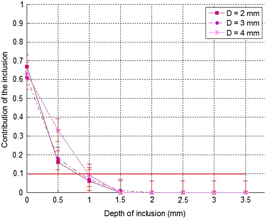
Leh et al.: Optical phantoms with variable properties and geometries for diffuse and fluorescence : : :

                phantom is not used for more than 1 h in a temperature-con-                        film is used between the inclusions and the surrounding gel. In
                trolled room at about 17°C.                                                        order to minimize the effect resulting from the migration of the
                                                                                                   inclusions’ fluorophores towards the surrounding gel and vice
                2.3     Phantoms—Geometrical Possibilities                                         versa, measurements on inclusion phantoms have been made
                                                                                                   within 10 min after inserting the inclusions.
                2.3.1    Mono-and bilayer phantoms

                A triangular-shaped mold (84 × 7 × 20 mm3 , see Fig. 3) can                        3       Data Analysis
                provide monolayer phantoms with a continued variation of
                                                                                                   All obtained fluorescence spectra are analyzed by home-written
                thicknesses. In addition, similar to those from Pfefer,31 bilayer
                                                                                                   Matlab programs. A typical spectrum measured from a bilayer
                phantoms can be produced using two triangular phantoms by
                                                                                                   phantom Stot is shown in Fig. 5. Stot corresponds to the weighted
                putting one onto the other to obtain a rectangular shaped 2-
                                                                                                   sum of two components: the emission spectrum of Rhodamine
                layer phantom [Fig. 4(b)]. Each of the layers—labelled with
                                                                                                   B, SRhB , and that of Fluorescein, SFITC . Background contribu-
                either Fluorescein or Rhodamine B—has its own specific set
                                                                                                   tions were already subtracted from the raw data.
                of optical parameters. A very thin (13 μm thickness) nonfluor-
                                                                                                       If more than one fluorophore was used, e.g., in case of
                escent film is placed in between the two layers to prevent fluor-
                                                                                                   bilayer phantoms or inclusion phantoms, the contribution of
                ophores from migrating into the other layer. Due to the flexible
                                                                                                   each fluorophore has to be determined. In a first step, a charac-
                texture of the gelatine phantoms, an almost perfect interface is
                                                                                                   teristic emission spectrum SRhB and SFITC of each utilized fluor-
                obtained, in most cases without any air bubbles. In contrast to
                                                                                                   ophore (n ¼ 4 for each fluorophore) has been measured using
                Pfefer’s phantoms having only two determined thicknesses (0.3
                                                                                                   monolayer phantoms with equivalent optical parameters and
                and 0.6 mm), in our case any thickness of the upper layer can be
                                                                                                   concentrations. These spectrum are averaged then modelled
                addressed as it depends only on the probe position.
                                                                                                   by weighted sums of Gaussians, two for Rhodamine B and
                                                                                                   three for Fluorescein, the Gaussian number chosen to obtain
                2.3.2    Phantom with cylindrical inclusions                                       the best correspondence measure/sum of Gaussian (coefficient
                A specific mold [Fig. 4(a)] was designed for phantoms with gel                     of adjusted >0.99). Every spectra of fluorophore is normalized
                inclusions, allowing a total of six cylindrical inclusions split into              by the area under the curve of the corresponding fluorophore. In
                two groups of three inclusions with 2, 3, and 4 mm diameters                       this way, the yield of fluorescence is corrected. Indeed, flower
                each. For the first group, the inclusions can be placed at a depth                 and f upper correspond respectively to the area under the curve
                D from 0 to 3 mm, whereas the second group is situated at a                        of the specter of Rhodamine B and the area under the curve
                depth of D þ 0.5 mm [Fig. 4(c)], with D being defined as                           of FITC corrected by the yield of the fluorescence. To simplify,
                the distance between the phantom surface and the closest                           these factors (f lower and f upper ) will be likened to fluorescence
                point of the cylinders to the surface. The phantom production                      intensity. These spectra were then used to fit the experimental
                procedure is done as follows: the gel inclusions are produced                      data from bilayer or inclusion phantoms, as presented in Eq. (2).
                in the horizontal cylindrical holes in the right part of the
                mold. The body of the phantom is molded in the rectangular
                                                                                                               StotðλÞ ¼ f lower SRhB ðλÞ þ f upper SFITC ðλÞ:          (2)
                shaped space on the left while aluminum cylinders are in
                place as illustrated for the first group of inclusions on Fig. 4
                (a). After gel polymerization, the aluminum cylinders are                             The result of this procedure is also shown in Fig. 5. The fitted
                taken out, leaving open spaces facing the gel inclusions in                        RhB (dashed line) and FITC (dotted line) contributions are
                mold. By using aluminum cylinders again, the gel inclusions                        shown with their sum (black line). This sum fits well the mea-
                can be pushed into the holes. The whole procedure is done                          sured data (grey dots).
                underwater to avoid creating air bubbles. The resulting phantom
                can be seen in Fig. 4(c). Contrary to the bilayer phantoms, no

                Fig. 3 Triangular home-designed mold used to make mono and bilayer
                phantoms.

                Fig. 4 (a) A picture of the mold designed to produce phantoms with
                cylindrical inclusions; Aluminium cylinders have been inserted into                Fig. 5 Measured spectrum from a bilayer phantom; fitted by its two
                the mold holes to illustrate the phantom fabrication. (b) Diagrams of              components RhB and FITC after subtraction of the contributions of
                bilayer phantom, and (c) inclusion phantom.                                        noise.

                Journal of Biomedical Optics                                               108001-4                                          October 2012   •    Vol. 17(10)

Downloaded From: https://www.spiedigitallibrary.org/journals/Journal-of-Biomedical-Optics on 19 Jun 2022
Terms of Use: https://www.spiedigitallibrary.org/terms-of-use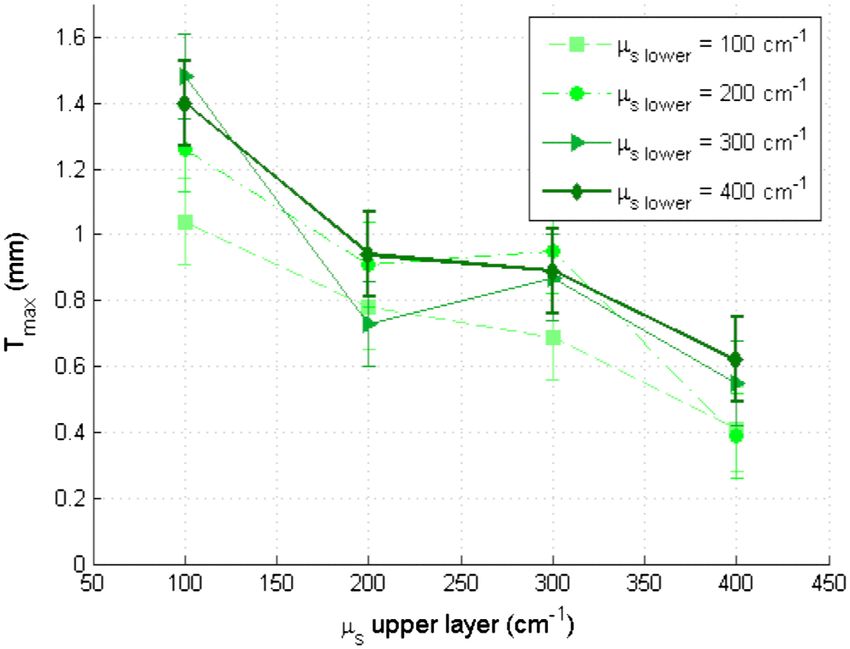
Leh et al.: Optical phantoms with variable properties and geometries for diffuse and fluorescence : : :

                    The specific labelling of the layers with different fluoro-                        The 10% value used to define detectability was arbitrarily
                phores allows for identification of the fluorescence origin                        chosen and real tissue tests will have to be performed to adjust
                and, at the same time, the relative contribution from each                         this value. But the 10% contribution value can provide a good
                layer or inclusion. Consequently, the layer thickness that can                     estimation to evaluate probes.
                be detected as a function of the different geometrical and optical                     T min corresponds to a contribution of 10% of the upper layer
                parameters of probe and phantom was estimated.                                     from the total recorded signal. It illustrates the capacity to detect
                    For a given probe-phantom distance, the fluorescence inten-                    a tumoral on-surface layer. If a layer has a superior thickness to
                sity is measured at each position corresponding to different                       T min it will be considered detectable. The coefficient T max is
                thicknesses (T) of the upper layer. The result is then divided                     equal to a thickness of the upper layer corresponding to a con-
                by the maximal fluorescence intensity collected from the super-                    tribution of 10% of the lower layer of the total collected signal.
                ior layer of the bilayer phantom (equivalent to a monolayer                        In that case, the tumoral layer is considered as being covered by
                phantom). This estimates the percentage of emitted fluorescence                    a healthy layer of tissue. If the healthy layer of tissue has a lower
                of the upper layer from a specific thickness. To compare the                       thickness of T max , the tumoral layer is detectable.
                different configurations, we defined a T 80% value that indicates
                the thickness of the upper layer that gives 80% of the detected                    4       Results
                light. In other words, in a monolayer phantom, about 80% of the                    Before use, the absorption and scattering coefficients of the
                detected light would come from this layer thickness.                               phantom have been experimentally verified with an integrating
                    Such obtained fluorescence intensities for each part or layer                  sphere and the obtained results matched the expected coeffi-
                of the phantom can be used to define the detectability of the                      cients. These measurements were accomplished for different
                layer. In consequence, all emissions of the different chromo-                      couples of (μs ,μa ).
                phores contributing to the total signal have to be taken into                          Figure 7 exposes the values of measured μs according to the
                account. The percentages P of the upper and lower layers are                       expected values (in agreement with Mie theory). Theoretical
                calculated with Eqs. (3) and (4), respectively and a typical exam-                 values are realized by the red line. The error bars shown in
                ple is given in Fig. 6.                                                            the following graphs had been always estimated using eight
                                                                                                   identical phantoms. These errors are estimated by the standard
                                                            f upper ðTÞ                            deviation between the measurements made for every scattering
                              Pupper layer ðTÞ ¼                                        (3)
                                                   f upper ðTÞ þ f lower ðTÞ                       coefficient. An overestimation of the scattering coefficient is
                                                                                                   observed with respect to what we expected, with an average rela-
                                                                                                   tive error of 15% and a maximal relative error of 23%.
                                                            f lower ðTÞ
                              Plower layer ðTÞ ¼                             :          (4)            In the phantom study, only one optical parameter of a layer
                                                   f upper ðTÞ þ f lower ðTÞ                       was varied, either the scattering or the absorption coefficient.
                                                                                                   While, the other parameters were always n ¼ 1.4, g ¼ 0.87
                                                                                                   and ðFluorophoreÞ ¼ 10−5 M. When varying μs ,μa was
                    We consider a layer detectable if it contributes to at least 10%               3 cm−1 . On the other hand, μs was 100 cm−1 , when the absorp-
                of the total signal. As P varies with the thickness of the layer, we               tion coefficient was changed.
                can therefore define two indicators, T min , which is the minimal
                thickness of the upper layer needed to be detected and T max ,
                                                                                                   4.1      Probe Positioning and Geometry
                which corresponds to the maximal thickness of the upper
                layer allowing the detection of the lower layer.                                   As shown in previous research, the position of the probe relative
                                                                                                   to the phantom plays an important role in terms of fluorescence
                                                                                                   light collection.16,31,32 In our case, we evaluated the optimal

                Fig. 6 The fluorescence contributions (P) of FITC (upper layer, black
                line) and RhB (lower layer, grey line) of a bilayer phantom. Data
                have been smoothed. The optical properties of both layers are the
                same, except for the fluorophore F∶n ¼ 1.4; μs ¼ 100 cm−1 ;                        Fig. 7 the values of measured μs according to the expected values (in
                g ¼ 0.87; μa ¼ 3 cm−1 ; ðFÞ ¼ 10−5 M.                                              agreement with Mie theory).

                Journal of Biomedical Optics                                               108001-5                                         October 2012   •   Vol. 17(10)

Downloaded From: https://www.spiedigitallibrary.org/journals/Journal-of-Biomedical-Optics on 19 Jun 2022
Terms of Use: https://www.spiedigitallibrary.org/terms-of-use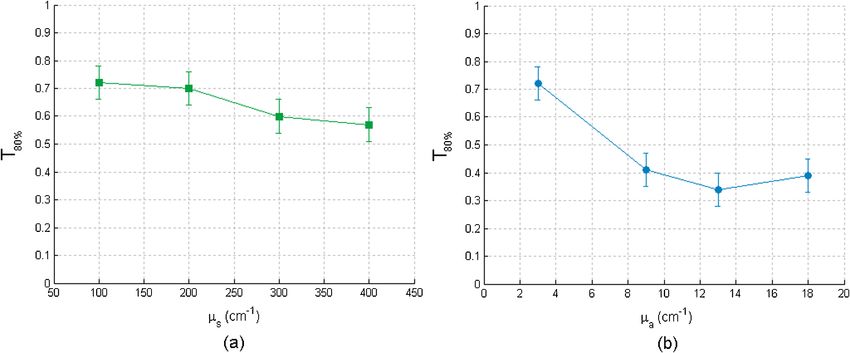
Leh et al.: Optical phantoms with variable properties and geometries for diffuse and fluorescence : : :

                                                                                                   Table 1 T 80% values for various scattering coefficients of monolayer
                                                                                                   phantoms.

                                                                                                   μs ðcm−1 Þ                                                       T 80%

                                                                                                   100                                                              0.53

                                                                                                   200                                                              0.57

                                                                                                   300                                                              0.62

                                                                                                   400                                                              0.50

                                                                                                   0.5 mm. This parameter does not seem to vary significantly
                                                                                                   according to μs and is about 0.56  0.05 mm, corresponding
                                                                                                   to the average and the standard deviation of the values presented
                                                                                                   in Table 1. A statistical error was evaluated by calculating the
                Fig. 8 Fluorescence intensity measured for several probe-sample
                                                                                                   standard deviation between the T 80% determined on several
                separation distances and scattering coefficients. The other optical prop-
                erties of the phantoms used for these measurements are: n ¼ 1.4;                   phantoms (n ¼ 8) with identical optical properties and was esti-
                g ¼ 0.87; μa ¼ 3 cm−1 ; ðRhBÞ ¼ 10−5 M.                                            mated to be 0.06 mm. This error is of the same order as the
                                                                                                   standard deviation of the values of Table 1, what strengthens
                                                                                                   the conclusion of independency between T 80% and μs .
                position by means of monolayer phantoms. Several phantoms                              For bilayer phantoms: In this case, the optical parameters of
                with different scattering coefficients were fabricated and the                     both layers are identical, except for the fluorophore. We view
                intensity of fluorescence light was measured as a function of                      two cases, the variation of the scattering coefficient and that
                the distance between the probe and the sample. As illustrated                      of absorption coefficient. A variation of μs , μa is fixed to
                in Fig. 8, for all μs the collected fluorescence intensities change                3 cm−1 and when μa is different, μs ¼ 100 cm−1 . Every
                considerably with the probe-sample distance. The shape of the                      point of the curve represents the average between two values
                curves is similar for all scattering coefficients. Qualitatively, this             of T 80% defined on two lines of measurements acquired on
                shape can be understood by the changing acceptance overlap of                      the same phantom; the average distance between these measure-
                the excited and collected fibers and the collection efficiency,                    ments for the different phantom is lower than 2%. The error bars
                both varying with distance. The highest fluorescence collection
                                                                                                   (0.06 mm) result from a standard deviation between eight
                yield is found at a probe-sample distance between 1.2 and
                                                                                                   values of effective penetration, calculated on eight phantoms
                1.5 mm. This is important for future clinical applications,
                                                                                                   of identical optical properties. Figure 9(a) shows the variation
                where a spacer will be necessary to position the probe correctly.
                                                                                                   of T 80% as a function of scattering coefficient and Fig. 9(b)
                    The error of the estimated probe-tissue distance is about
                                                                                                   as a function of absorption coefficient.
                0.2 mm, mainly due to limited precision in measuring this dis-
                                                                                                       To determine if the effective depth of detection varies with μs
                tance (flatness of probe and phantom support). Accordingly, the
                                                                                                   or μa, we compared the standard deviation of the points of the
                distance used between the probe and the phantom was always
                1.5 mm within this study. It should be noted that this distance is                 curve, S80% with the square of the statistical error,
                specific for our probe characteristics. Consequently, the 1.5 mm                   σ 80% ¼ 0.06 mm, corresponding to 95% of confidence interval
                distance has to be changed when the probe geometry is modi-                        (a Shapiro test was used). If the criterion presented in Eq. (5) is
                fied, especially when the distance between emitting and collect-                   validated, then T 80% depends on the varied coefficient in the
                ing fiber is varied as this which affects the collection                           considered curve.
                acceptance.31
                                                                                                                         rffiffiffi n
                                                                                                                          1 X ðiÞ
                4.2     Sample and Layer Thicknesses                                                            S80%   ¼        ðT  − T 80% Þ ≥ 2:σ 80% :             (5)
                                                                                                                          n i¼1 80%
                The collected fluorescence intensity changes with the thickness
                of the sample. This can easily be measured with a triangular-
                shaped layer [Figs. 3 or 4(b)], where the sample thickness
                only depends on the position of the probe. This can be seen
                in Fig. 6, where a saturation effect is observed. What is more                         By applying this method, we find that, for Fig. 9(a), S80% ¼
                interesting; these kind of well-calibrated phantoms can be                         0.08 mm is lower than 2. σ 80% ¼ 0.12 mm, we cannot thus con-
                used to evaluate precisely the spatial origin of the fluorescence                  sider that the depth of detection varies with the scattering coeffi-
                emission.                                                                          cient. This conclusion is added to that made on the monolayer
                    For monolayer phantoms (n ¼ 4), Table 1 shows the esti-                        phantom. Concerning Fig. 9(a), the corresponding point in μa ¼
                mated thickness where 80% of the signal comes from, corre-                         3 cm−1 is statistically different from others, making them not
                sponding to four different scattering coefficients. We observe                     differentiated. We can conclude that the effective depth of detec-
                that even for a high-scattering medium, this penetration depth                     tion does not vary with μs but depends on μa . For an absorption
                only marginally changes. In conclusion, we estimated the thick-                    coefficient (μa ) of 3 cm−1 , T 80% is about 0.65  0.08 mm, and
                ness of the explored bulk by our system to be typically around                     decreases to a value of 0.38 mm for higher μa.

                Journal of Biomedical Optics                                               108001-6                                         October 2012   •   Vol. 17(10)

Downloaded From: https://www.spiedigitallibrary.org/journals/Journal-of-Biomedical-Optics on 19 Jun 2022
Terms of Use: https://www.spiedigitallibrary.org/terms-of-use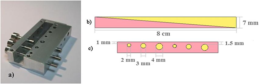
Leh et al.: Optical phantoms with variable properties and geometries for diffuse and fluorescence : : :

                                Fig. 9 Variation of the depth of detection of 80% of the signal of the superior layer according to μs (a) and of μa (b).

                4.3     Detectability                                                              fixed scattering coefficient of the upper layer and variable scat-
                                                                                                   tering coefficient of the lower layer. In Table 2(b), it is the μs of
                In this case, the optical coefficients of the upper and lower layers               the upper layer which is changed while the μs of the lower layer
                are not always identical. These new analyses aim at bringing                       is fixed.
                information about the capacity of the probe to detect the one
                                                                                                       By comparing the values of Table 2 to the critical value σ max ,
                or the other layer of both superimposed different layers.
                                                                                                   we can deduce that the maximal thickness of detection does not
                These results will be approached by the detection of a tumoral
                                                                                                   depend on the scattering coefficient of the lower layer, but it is
                surface layer or in-depth.
                                                                                                   influenced by the scattering properties of the upper layer. The
                     The maximum thickness T max of the upper layer allowing the
                                                                                                   more scattering the upper layer has, the less the thickness T max
                detection of the lower layer has been measured for different μs
                                                                                                   will be, with average values included between 1.3 and 0.49 mm.
                and μa . As can be seen in Fig. 10, a study of the maximal thick-
                                                                                                   A high scattering corresponds to a low mean free path in tissues.
                ness of the upper layer according to μs of the upper layer was
                                                                                                   If we consider an average number of steps of scattering identi-
                made when the absorption coefficient is fixed to 3 cm−1 Every
                                                                                                   cal, whatever μs, a photon will penetrate less deeply in tissue
                curve corresponds to a fixed μs of the lower layer.
                                                                                                   with higher scattering coefficient. This can explain qualitatively
                     A criterion identical to that presented in Eq. (5) was used to
                define if the observed variation was significant or not. In that                   the decrease of T max for higher μs.
                case, the critical value is 2. σ max ¼ 0.26 mm and the standard
                deviation Smax is calculated for values T max according to fixed                   Table 2 Standard deviation Smax for fixed μs of the upper (a) and lower
                μs , either for the lower or upper layer. Table 2 present the values               (b) layer.
                of Smax . Table 2(a) contains the values of Smax calculated for a

                                                                                                   (a)

                                                                                                   Fixed μs upper layer (cm−1 )                                  S max (mm)

                                                                                                   100                                                              0.19

                                                                                                   200                                                              0.10

                                                                                                   300                                                              0.11

                                                                                                   400                                                              0.11

                                                                                                   (b)

                                                                                                   Fixed μs lower layer (cm−1 )                                  S max (mm)

                                                                                                   100                                                              0.29

                                                                                                   200                                                              0.36

                Fig. 10 Variation of the maximal thickness of upper layer allowing the             300                                                              0.40
                detection of the lower layer according to different scattering coefficient
                                                                                                   400                                                              0.32
                of both layers. μa is 3 cm−1 .

                Journal of Biomedical Optics                                               108001-7                                          October 2012    •   Vol. 17(10)

Downloaded From: https://www.spiedigitallibrary.org/journals/Journal-of-Biomedical-Optics on 19 Jun 2022
Terms of Use: https://www.spiedigitallibrary.org/terms-of-use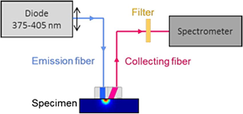
Leh et al.: Optical phantoms with variable properties and geometries for diffuse and fluorescence : : :
Fig. 11 Variation of the maximal thickness of upper layer allowing the detection of the lower layer according to different absorption coefficient of both
layers.
For various scattering and absorption coefficients, the T min we can observe a decrease of T max with μa of the upper
value is always found less than 60 μm. An error was also esti- layer for small values of μa of the lower layer, as seen in Fig. 11.
mated by using identical bilayer phantoms. The estimated T min The deducted values of T min are always lower than 70 μm for
error is 20 μm. taking into account this error, the upper layer different μa , for an average value of 30 μm.
will always be detected, if its thickness is at least 80 μm. Note that in the case of cancer tissue that has necessarily a
Optical problems in tissues are especially difficult regarding higher μs underneath healthy tissue, the explored thickness is
scattering and absorption. For this reason, a study similar to that between 1.3 and 0.5 mm (Table 2).
of the variation of μs was made by varying the absorption coef- We conclude that T max depends on the μs of the upper layer
ficient μa . Figure 11 present results of T max according to μa of and is not affected by the variation of μs and μa of the
the upper layer, where each curve corresponds to a fixed μa of lower layer.
the lower layer. The standard deviation Smax is also calculated in Further study and measurements will be accomplished to
these cases and the results are recapitulated in Table 3. evaluate this thickness for tissues combining high scattering
We cannot conclude the existence of any dependence of the and high absorption coefficients.
thickness T max on the absorption coefficient in the range
included between 3 and 18 cm−1 from Table 3. Qualitatively, 4.4 Phantoms With Inclusion
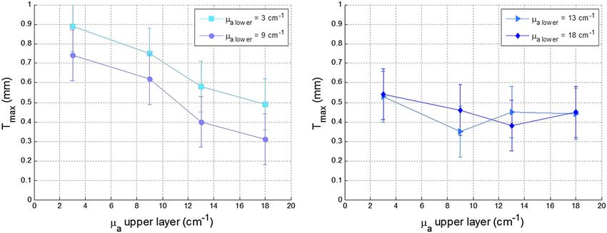
The use of inclusion phantoms [Fig. 4(c)] allows the analysis of
Table 3 Standard deviation Smax for fixed μa of the upper (a) and lower very local “tissue” modifications and to evaluate its fluorescence
(b) layer. contribution to the whole detected signal, which depends on its
size and depth within the phantom. Evidently, optical para-
(a) meters can be varied as well. The probe is moved across
these phantoms similarly to the bilayer phantoms and the mea-
Fixed μa upper layer (cm−1 ) S max (mm) sured data are fitted in the same way.
A typical result can be seen in Fig. 12. Fluorescence inten-
3 017 sities of FITC inclusions are shown as a function of the x-axis
position of the scan when the probe is displaced laterally across
9 0.17
the phantom. Each peak has already been fitted with a Gaussian
13 0.09 curve to get position and full width at half maximum (FWMH)
of the inclusion.
18 0.07 Several phantoms were built to cover a range of inclusion
depths between 0 and 3.5 mm. Figure 12 presents the variation
(b)
of the detected intensity maximum as a function of this depth.
Squares, circles and triangle represent 2-, 3- and 4-mm diameter
Fixed μa lower layer (cm−1 ) S max (mm)
inclusions, respectively.
The parameters of interests are the maximum and the
3 0.16 FWHM. The error on the maximal intensity measured on an
9 0.20 inclusion was calculated by means of six phantoms each one
contain six inclusions, half in 1 mm depth and the others
13 0.07 1.5 mm deep. The average variation of the maximal intensity
was estimated with a relative standard deviation of the order
18 0.07 of 1%, with a maximal standard deviation of 3%.
Journal of Biomedical Optics 108001-8 October 2012 • Vol. 17(10)
Downloaded From: https://www.spiedigitallibrary.org/journals/Journal-of-Biomedical-Optics on 19 Jun 2022
Terms of Use: https://www.spiedigitallibrary.org/terms-of-useLeh et al.: Optical phantoms with variable properties and geometries for diffuse and fluorescence : : :
Table 4 Average values of FWHM for different diameters.
Diameter (mm) FWHM (mm)
2 1.3 0.5 (n ¼ 4)
3 1.8 0.2 (n ¼ 4)
4 2.4 0.2 (n ¼ 4)
developed to evaluate the detection properties. To achieve
this study, we took into account various thicknesses or depths,
inclusions of several sizes and optical parameters. In case of a
monolayer phantom, the thickness T 80% from where 80% of the
total signal is collected, is independent of the scattering coeffi-
Fig. 12 FITC intensity as a function of probe position. The optical prop-
erties of the FITC inclusions are: n ¼ 1.4; μs ¼ 150 cm−1 ; g ¼ 0.87;
cient and is around 0.56 0.06 mm.
μa ¼ 3 cm−1 ; ðFITCÞ ¼ 10−5 M. The surrounding gel has the same para- When considering bilayer phantoms, two different indica-
meters except for the scattering coefficient μs ¼ 100 cm−1 and the fluor- tors, T min and T max , were investigated corresponding to the
ophore, which is RhB. The inclusion depths are 1 and 1.5 mm. minimal and maximal thicknesses of the upper layer that still
permits detection of the upper or lower layer, respectively.
For both indicators, absorption and scattering coefficients
have been varied.
Figure 13 recapitulates the maxima of the inclusions’ contri- Being independent of absorption and scattering coefficients,
butions for different depths and diameters. The contributions in the minimum thickness T min of the upper layer to be detected is
0 mm depth are lower than 100%. This is understandable by the never larger than 80 μm and in most cases even smaller. On the
spatial resolution of the probe which is 500 μm and thus it mea- other hand, the maximum thickness of the upper layer allowing
sures a superior surface of the outcrop of the inclusion. The red detection of the lower layer is strongly μs –dependent. For
line represents the limit of 10% detectability. The detection is increasing scattering coefficient of the upper layer, T max
quasi-independent from the diameter of the inclusions, when decreases. In consequence, even a rather thin layer of tumorous
it is included between 2 and 4 mm. The maximal depth of tissue at the surface having a high-scattering coefficient will
the inclusion allowing its detection is about 0. 9 mm. inhibit a signal contribution from underlying healthy tissue,
The FWHM does not vary with the depth of the inclusion. property that should help in tumorous tissue identification.
Table 4 contains the average values of FWHM for different dia- More generally it can be stated that high differences of the scat-
meters. The relationship between FWHM and the diameter is tering coefficients of two tissue layers favor the detection of the
constant with a ratio of about 0.6. high diffusive tumorous one.
Detectability of inclusions has also been examined. At least
5 Discussion for inclusion diameters larger than 2 mm, the inclusions are
Using our homemade probe, several scattering, absorbing and detectable to depths of 1.5 mm. While the detectability does
fluorescent phantoms with different geometries have been not vary with diameter, the inclusion widths (FWHM) are under-
estimated by about 40%. Both properties can be explained by
geometrical considerations: the inclusions have a circular, not
a rectangular shape, and the determined depth is the distance
between the phantom surface and the inclusion’s top edge.
We determined the limit of detection, defined as a minimal con-
tribution of 10% of the measured total signal, in a depth slightly
lower than 1 mm. Nevertheless, the signal resulting from inclu-
sions is very well defined because of the adjustment method of
the emission spectrum and the same for superior depths. The
value of the threshold of detection defined arbitrarily in 10%
of the total signal seems too radical. In fact, it is possible,
due to the method of spectrum processing, to detect inclusions
more profoundly than the defined threshold.
6 Conclusion
In the present work, the making of original mono-and bilayer
phantoms, as well as phantoms with inclusions, was presented.
These phantoms with calibrated and verified optical parameters
are suited to fluorescence spectroscopy. They provide an accu-
Fig. 13 Normalized maximum peak intensities measured for inclusions rate tool to characterize and compare fiber probe detection char-
of 2, 3, and 4 mm diameters, corresponding to squares, circles and tri- acteristics. The phantom optical parameters have been fitted to
angles, respectively, as a function of the inclusion depth. mimic healthy and tumorous brain tissues. These phantoms are
Journal of Biomedical Optics 108001-9 October 2012 • Vol. 17(10)
Downloaded From: https://www.spiedigitallibrary.org/journals/Journal-of-Biomedical-Optics on 19 Jun 2022
Terms of Use: https://www.spiedigitallibrary.org/terms-of-useLeh et al.: Optical phantoms with variable properties and geometries for diffuse and fluorescence : : :
also well fabricated to be excited with 405 nm, a wavelength 12. A. N. Yaroslavsky et al., “Optical properties of selected native and coa-
frequently used for autofluorescence measurements of tissues. gulated human brain tissues in vitro in the visible and near infrared spec-
tral range,” Phys. Med. Biol. 47(12), 2059–2073 (2002).
In the end, the benefits of a phantom with variable optical
13. G. Wagnières, W. Star, and B. C. Wilson, “In vivo fluorescence spectro-
parameters and adaptable geometries were shown for detec- scopy and imaging for oncological applications,” Photochem. Photo-
tion-probe characterization. However, phantom studies are biol. 68(5), 603–632 (1998).
quite time-consuming. Complementary ways to validate probes 14. D. Abi-Haidar et al., “Spectral and lifetime domain measurements of rat
include Monte Carlo simulations that can be easily used to make brain tumors,” Proc. SPIE 8207, 82074P (2012).
a systematic characterization of different probe geometries. We 15. M. H. Vu Thi et al., “Intra-operative probe for brain cancer: feasibility
have developed such a simulation program and its validation via study,” Proc. SPIE 6628, 66281Q (2008).
16. M. H. Vu Thi, “Développement d’une sonde per-operatoire basée sur la
phantom measurements is under study.33 Detailed results will be détection d’autofluorescence pour l’assistance au traitement chirurgical
published soon. des tumeurs cérébrales,” Ph.D. thesis Université Paris XI (2008).
17. T. K. Biswas and T. M. Luu, “In vivo MR measurement of refractive
Acknowledgments index, relative water content and T2 relaxation time of various brain
lesions with clinical application to discriminate brain lesion,” Int. J.
The authors gratefully acknowledge the AnBioPhy laboratory Radiol. 13(1) (2011).
for letting them use their spectrophotometer, especially Imène 18. C. F. Bohren and D. R. Huffman, Absorption and Scattering of Light by
Chebbi for her welcome and help. This work is supported by Small Particles, Wiley, New York (1983).
Paris Diderot University (BQR). 19. S. Prahl, http://omlc.ogi.edu/software/.
20. M. Born and E. Worlf, Principals of Optics, 6th ed., Pergamon Press,
Oxford (1980).
References 21. H. C. Van de Hulst, Light Scattering by Small Particles, Wiley, New
York (1964).
1. F. W. Esmonde-White et al., “Biomedical tissue phantoms with con- 22. W. J. Lentz, “Generating Bessel functions in Mie scattering calculations
trolled geometric and optical properties for Raman spectroscopy and using continued fraction,” Appl. Opt. 15(3), 668–671 (1976).
tomography,” The Analyst 136(21), 4437–4446 (2011). 23. A. Ishimaru and Y. Kuga, “Attenuation constant of a coherent field in a
2. B. W. Pogue and M. S. Patterson, “Review of tissue simulating phan- dense distribution of particles,” J. Opt. Soc. Am. 72(10), 1317–1320
toms for optical spectroscopy, imaging and dosimetry,” J. Biomed. Opt. (1982).
11(4), 041102 (2006). 24. A. Lagendijk and B. A. van Tiggelen, “Resonant multiple scattering of
3. G. C. Beck et al., “Design and characterisation of a tissue phantom sys- light,” Phys. Rep., 270, 143–215 (1996).
tem for optical diagnostics,” Laser Med. Sci. 13(3), 160–177 (1998). 25. B. Gélébart et al., “Phase function simulation in tissue phantoms: a frac-
4. K. P. Rao, S. Radhakrishnan, and M. R. Reddy, “Brain tissue phantoms tal approach,” Pure Appl. Opt. 5(4), 377–388 (1996).
for optical near infrared imaging,” Exp. Brain Res. 170(4), 433–437 26. S. L. Jacques, “Short course note: tissue optics,” SPIE Education
(2006). Courses (2012).
5. L. T. Nieman, M. Jakovljevic, and K. Sokolov, “Compact beveled fiber 27. F. Martelli et al., Light Propagation Through Biological Tissue and
optic probe design for enhanced depth discrimination in epithelial tis- Other Diffusive Media: Theory, Solutions, and Software, p. 193,
sues,” Opt. Express 17(4), 2780–2796 (2009). SPIE Press Monograph, San Jose (1970).
6. K. Vishwanath and M. A. Mycek, “Time-resolved photon migration in 28. L. Henyey and J. Greenstein, “Diffuse radiation in the galaxy,” Astro-
bi-layered tissue models,” Opt. Express 13(19), 7466–7482 (2005). phys. J. 93, 70–83 (1941).
7. D. Kepshire et al., “Fluorescence tomography characterization for sub- 29. S. Jacques et al., “Specifying tissue optical properties using axial depen-
surface imaging with protoporphyrin IX,” Opt. Express 16(12), 8581– dence of confocal reflectance images: confocal scanning laser microscopy
8592 (2008). and optical coherence tomography,” Proc. SPIE 6446, 64460N (2007).
8. M. A. Ansari, R. Massudi, and M. Hejazi, “Experimental and numerical 30. D. Abi-Haidar and T. Oliver, “Confocal reflectance and two-photon
study on simultaneous effects of scattering and absorption on fluores- microscopy studies of a songbird skull for preparation of transcranial
cence spectroscopy of a breast phantom,” Opt. Las. Technol. 41(6), imaging,” J. Biomed. Opt. 14(3), 034038 (2009).
746–750 (2009). 31. T. J. Pfefer et al., “Selective detection of fluorophore layers in turbid
9. I. Noiseux et al., “Development of optical phantoms for use in fluores- media: the role of fiber optic probe design,” Opt. Lett. 28(2), 120–
cence-based imaging,” Proc. SPIE 7567, 75670B (2010). 122 (2003).
10. Q. Liu, G. Grant, and T. Vo-Dinh, “Investigation of synchronous fluor- 32. T. Papaioannou et al., “Effects of fiber-optic probe design and probe-to-
escence method in multicomponent analysis in tissue,” IEEE J. Sel. Top. target distance on diffuse reflectance measurements of turbid media: an
Quantum Electron 16(4), 927–940 (2010). experimental and computational study at 337 nm,” Appl. Opt. 43(14),
11. S. C. Gebhart, W. C. Lin, and A. Mahadevan-Jansen, “In vitro determi- 2846–2860 (2004).
nation of normal and neoplastic human brain tissue optical properties 33. B. Leh et al., “Development of an autofluorescence probe far brain can-
using inverse adding-doubling,” Phys. Med. Biol. 51(8), 2011–2027 cer: probe characterization thanks to phantom studies,” Proc. SPIE
(2006). 7567, 756707 (2010).
Journal of Biomedical Optics 108001-10 October 2012 • Vol. 17(10)
Downloaded From: https://www.spiedigitallibrary.org/journals/Journal-of-Biomedical-Optics on 19 Jun 2022
Terms of Use: https://www.spiedigitallibrary.org/terms-of-useYou can also read