Near Real-Time Social Distancing in London
←
→
Page content transcription
If your browser does not render page correctly, please read the page content below
Near Real-Time Social Distancing in London

                                         James Walsh1 , Oluwafunmilola Kesa2 , Andrew Wang4 , Mihai Ilas4 , Patrick O’Hara2 , Oscar
                                                               Giles1 , Neil Dhir1,2 , Theodoros Damoulas1,2,3
                                                                            1
                                                                              The Alan Turing Institute
                                                                  {jwalsh, ogiles, ndhir}@turing.ac.uk
arXiv:2012.07751v2 [cs.CY] 19 Apr 2021

                                                      Departments of 2 Computer Science and 3 Statistics, University of Warwick
                                                      {funmi.kesa, patrick.h.o-hara, t.damoulas}@warwick.ac.uk
                                                               4
                                                                 Engineering Department, University of Cambridge
                                                                         {aslw3, mai32}@cam.ac.uk

                                                                                      Abstract

                                                  During the COVID-19 pandemic, policy makers at the Greater London Authority,
                                                  the regional governance body of London, UK, are reliant upon prompt and accurate
                                                  data sources. Large well-defined heterogeneous compositions of activity throughout
                                                  the city are sometimes difficult to acquire, yet are a necessity in order to learn
                                                  ‘busyness’ and consequently make safe policy decisions. One component of our
                                                  project within this space is to utilise existing infrastructure to estimate social
                                                  distancing adherence by the general public. Our method enables near immediate
                                                  sampling and contextualisation of activity and physical distancing on the streets of
                                                  London via live traffic camera feeds. We introduce a framework for inspecting and
                                                  improving upon existing methods, whilst also describing its active deployment on
                                                  over 900 real-time feeds.

                                         Introduction

                                         Sources of public data regarding the current global pandemic fail to meet a number of requirements:
                                         accuracy in recorded measure, spatial and temporal granularity, and most importantly accessibility to
                                         policy makers and the general public. As the global community is actively engaged in understanding
                                         more about the effects and transmission mechanism of COVID-19, many governments are enacting
                                         temporary restrictions targeted at reducing the proximity of the public to one another (i.e. ‘social
                                         distancing’). These have become known as “lock-downs" [16], and the monitoring of public response
                                         to these measures have come out of necessity for policy makers to better understand their adoption,
                                         plan economic recovery and eventual suspension. When social restrictions were first implemented in
                                         the UK there were limited options to measure activity. A number of private companies trading in
                                         public movement data began providing aggregate information at the request of local government, from
                                         sources such as workplace reporting, wearable sports activity trackers and point of sale transactions.
                                         It became clear there was an immediate need for additional response metrics for activity, unmet in
                                         the aforementioned sources. Here, we describe a social-distancing estimation system using Open
                                         Government Licensed [9] traffic cameras directed towards pedestrian crossings and pavements,
                                         reporting to policy makers in near real-time. This work includes the description of our pipeline
                                         and new accuracy results on urban footage benchmarks. Due to the nature of this work, there are
                                         substantial privacy concerns, all footage employed is anonymised through restrictive sampling and
                                         systematically undergoes continuous review by our organisation’s Ethical Advisory Panel.

                                         Preprint. Under review.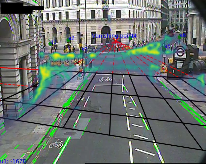
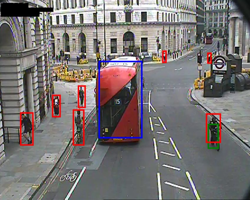
(a) Estimated ground plane from camera calibra-   (b) High accuracy detections, pedestrians, buses
tion, overlaid pedestrian detection density       and bicycles in red, blue, green respectively
           Figure 1: Example of our method applied to a traffic camera at Bank, London

Method
Our method starts with the calibration of each camera we expect to receive samples from, this
Camera Calibration is a one-time process to learn parameters for mapping from the 2D scene to a
3D real-world representation. Once complete, active data collection occurs continuously to ingest
samples from the public domain, upon successful retrieval each clip is queued for object detection
by the inference cluster. Upon exiting the detection stage, each pedestrian detection is transformed
to the learned world-plane representation. These results are submitted to the database, upon which
other digital twin components will be simultaneously retrieving and processing to watch for spikes or
irregularities in selected areas of concern.
1 Camera Calibration Obtaining a world-plane mapping of a camera scene is extensively de-
scribed in the computer vision literature. A large portion of literature requires manual calibration
using known patterns to estimate the transformation [2, 7, 23]. Vanishing line estimation is essential
for perspective transformation [4]. [18, 6] use the activity of a large number of vehicles travelling
parallel and regularly to find the vanishing point. [10, 22, 5, 8] calibrate the camera using clear,
regular or known lines in the scene, which is not practical for the case of a large spread of different
cameras. The stratified transformation discussed in [11] relies on the fact that there are many lines to
be extracted from high quality images to build a real-world model. [18], [22], [5] and [3] extract visi-
ble road features by using a derivative-based binarisation operator. This is only suitable for cameras
overlooking straight and visually similar lanes. Overall, our method is more easily generalised to
higher quantity of cameras with cluttered urban traffic scenes and lower resolution.
The mapping, (u, v, 0) 7→ (X, Y, Z), from the image plane to world geometry is sought, where there
is no a priori truth of the camera parameters. The intrinsics (focal length, principal point, skew
and aspect ratio) and extrinsics (positioning and direction) therefore must be estimated or assumed.
The cameras have the following limitations: Roads have non-zero curvature or have junctions and
vary in width; Irregular road markings of varying quality; Cameras have low resolution, changing
lighting in very short sample duration. To maintain robustness we make the following internal
camera assumptions: (a) unit aspect ratio and constant skew; (b) coincidence of principal point
and image centre; these are commonplace and rarely estimated due to lack of visual information
[4], [6]. External assumptions are as following; (c) zero radial distortion; (d) flat horizon v0 = v1 ;
(e) zero-incline road Z = 0; these seem reasonable by manual inspection of 100 random cameras
and must be made given the above limitations. If cameras where these assumptions do not hold, a
pre-processing stage using additional information can be implemented to correct radial distortion [6],
inclined horizon (setting v1 6= v0 ), and non-zero inclination Z [19].
This simplified pinhole camera model allows the transformation to be described by four parameters
u0, v0, u1, h where (u0, v0), (u1, v0) are the vanishing points of two orthogonal planar directions
subtending the horizon line, and h is the height of the camera above ground (Figure B.1). Parallel
lines on the road and on cars, such as road edges, advanced stop lines and car and truck edges, are
used to estimate this transformation (Figure 2).

                                                   2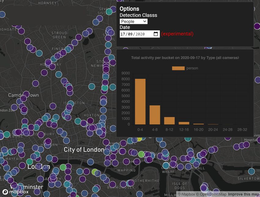
Figure 2: Lines detected by our feature extraction algorithm, two orthogonal sets of lines: those
parallel to the foreground road (green, road edges) and those perpendicular (blue, road perpendicu-
lars). The intersection of each set, the vanishing point (light blue) which lies on the horizon. The
challenging conditions are shown here, including varying lighting and non-zero road curvature.
The Canny edge detector [21] is applied per frame to find sets of road edges and road perpendiculars
as shown in Figure 2. The Hough transform matches collinear edge segments into linked lines
which are then filtered by gradient[18] and dimensions. The vanishing point is then simply the
maximum histogram density estimate of the pairwise line intersections. This is chosen over more
expensive MLE methods [24] where the vanishing point error is optimised using least squares [4],
[3] or Levenberg–Marquardt [18], [11]. This procedure is repeated across different contrast factors
to provide a robust line detector in challenging lighting conditions. Finally, u0 , u1 , v0 values are
averaged over all frames to extract maximum information when the videos are sparsely populated
with vehicles. Finally, the camera height h can be manually calculated by transforming an object of
known dimensions. For example, using frequently appearing London buses of fixed 2.52m width, the
calculated height averages h = 9.6m with 10% average deviation across 7 randomly picked cameras.
Other ways to obtain the scale h include using car length averages [19] or known lane spacings [8, 3].
2 Data Collection Transport for London (TFL) sourced footage selected for this platform consists
of ten-second videos from 911 live cameras every four-minutes from the Open Roads initiative, known
as JamCams [15]. A day of collection constitutes 220,000 individual files of a total of 20-30GB,
deleted upon processing in accordance with our data retention policy. The nature of monitoring public
spaces means we cannot a priori request consent. We limit the resolution of our collected footage to
inhibit any capacity to personally identify an individual. Thus only their humanoid likeness is utilised
for detection.
3 Object Detection In order to detect entities quickly Kingsland Rd/Ball Pond Rd
●
enough to assist policy makers, we evaluated object de- 20 ●
● ●
●
●
● ● ●
tection models such as SSD[13], YOLO v3[17] & YOLO 15
● ● ●
●
●
●
v4[1] to balance speed with accuracy. These are typi- ● ●
● ●
● ● ●
●
●
● ● ●●
●
●
●
●
●
● ●
● ● ●
Count
● ● ● ● ● ● ●
cally determined by architecture, model depth, input sizes, 10 ●
●
● ●
●
●
● ● ●
●●
● ●●
●
●
●
● ●
● ●
●
● ● ●
● ●
● ●● ● ● ●● ● ● ● ● ●
classification cardinality and execution environment. You ●
● ● ●
● ●
●
●●●●●●
●● ● ●● ● ●●
● ●● ● ● ● ●
●
●
● ●
●● ●
● ● ●
● ●●
● ●●
● ● ●●
● ● ●
●●
5 ● ●● ●
●
● ●● ● ● ● ● ● ●
Only Look Once (YOLO) is a one-stage anchor-based ●
●
●●
●
● ● ●● ●
● ●
● ●
● ● ●
●● ● ●
●
● ●
●●● ●
●●
● ●
●
●
● ● ●
● ●
● ● ●● ●●
● ●
●
●
●
●
●
●
●
●● ● ● ●● ●● ● ● ● ● ● ● ● ●
object detector that is both fast and accurate. YOLOv3 0
achieves an accuracy of 57.9 AP50 in 51ms [17]. Re-
Jun 01 Jun 08 Jun 15 Jun 22 Jun 29
cently, a faster version named YOLOv4, was released with Date
a state-of-the-art accuracy than alternative object detectors. Figure 3: Pedestrians in samples from
Notably, YOLOv4 can be trained and used on conventional Kingsland Rd/Ball Pond Rd, June 2020
GPUs which allows for faster experimentation and fine-
tuning on custom datasets. YOLOv4 improves performance and speed by 10% and 12% respectively
[1]. We employ both YOLOv3 & v4 in our experiments. Each were pretrained on Coco[12] dataset,
a large-scale repository of objects belonging to 80 class labels. Due to our objective, the classes of
interest are limited to six labels: person, car, bus, motorbike, bicycle, and truck. We fine-tuned the
model on six labels using joint datasets from COCO and MIO-TCD[14], and then evaluated them
against. Results in the evaluation section shows that fine-tuning the traffic camera footage.
3
Datasets     person    bicycle      car     motorbike      bus      truck
                    Coco 2017   262 465       7113     43 867       8725       6069      9973
       Train
                    MIO-TCD       5760        1758    186 767       1484       8443     54 340
                    Coco 2017    11 004        316      1932         371        285        415
       Validation   MIO-TCD       1368         502     46 730        353       2155     13 694
                    Jamcam        1233         106      7867         106        203      1982

                         Table 1: Training and Validation Dataset Statistics

4 Social distancing To measure distance within this scene we may find the Eu-
clidean distance between pedestrian detections after the above world plane pro-
jection.      We elected to improve in areas of high pedestrian use by employing
points of reference via geotagged static urban furniture, such as traffic lights.
We first select an appropriate flat 2D projected co- "x0 + e # " k cos(θ) k sin(θ) t # "x#
                                                              x        1              3           x
ordinate reference system, British National Grid       y 0 + ey = −k2 sin(θ) k4 cos(θ) ty y
(OS 27700). Then, we create a second transfor-             0              0             0        1     0
mation between these two 2D Cartesian frames of
reference, represented below with scale and shear factors, k, angle of rotation, θ, translations t, and
error terms, e. The estimated real world plane is then generated from the optimisation of the sum of
squares error.

Evaluation
Camera calibration Uncertainty in the estimation of
the vanishing line and extrinsic camera height arises due
to imperfect camera effects eliminated in the assumptions
and inaccurate automatic line extraction. The estimated er-
rors in mapped world position dX, dY , are evaluated for 3
randomly selected cameras which are manually calibrated
beforehand using the total differential over all estimated
parameters pi ∈ {u0 , v0 , u1 , h} assuming that the vehicle
tracking u, v are accurate at the point of evaluation. The
average relative uncertainty in position mapping due to
parameter estimation | dX
                        X | is calculated to be 17.7%, σ = Figure 4: Estimated locations of urban
7.9%.                                                        furniture (green) and pedestrians (blue)
                                                             on British National Grid
Object detection As preprocessing steps, we subset 6
labels from the Coco 2017 and MIO-TCD localization dataset. Unlike the Coco dataset, MIO-TCD
localization dataset contains 11 labels with additional categories such as motorized vehicle, non-
motorized vehicle, pickup truck, single unit truck, and work van, not found in the Coco 2017 dataset.
For comparison, we collapse the different categories of trucks as truck and remove labels regarding
vehicle motorization. We produced new collection of manually labelled entities specifically on frames
from traffic cameras, using CVAT [20]. The dataset contains 1142 frames and 11497 bounding boxes
as shown in Table 1. For evaluation/validation, we compute the mean Average Precision (mAP) at
IOU threshold of 0.5 over the Coco 2017, MIO-TCD, joint (Coco 2017 + MIO-TCD), and JamCam
datasets.
We fine-tune a pretrained YOLOv4 weights file on six labels from different training datasets using a
batch size of 16, subdivsions of 4, image size of 416 and at least 7000 iterations on a Tesla V100-
SXM3-32GB GPU. We train three different models on 1) Coco 2017 training data 2) MIO-TCD
training data 3) Joint data containing random shuffle of Coco 2017 and MIO-TCD training data. Table
1 shows the number of training data by labels. The validation data contains Coco 2017 validation
data, MIO-TCD validation data and Jamcam data.
The performances of the three models are shown in Table 2. On the Coco 2017 validation data, the
model achieves a mean Average Precision (mAP@0.50) of 67.55 %. However, the model trained
on Coco 2017 dataset performed poorly on MIO-TCD localization validation dataset with an mAP
of 20.39 %. Likewise, the performance of the model trained on MIO-TCD dataset reduces greatly
from 85.80 % to 14.24 % when Coco 2017 dataset is used as the validation dataset. This behaviour

                                                  4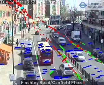
Training    Validation mAP@0.50 ↑ Precision ↑ Recall ↑ F1-score ↑
                            Coco           67.55        0.73       0.70      0.71
                Coco        MIO-TCD        20.39        0.38       0.49      0.43
                            JamCam         41.64        0.62       0.59      0.60
                        Coco               14.24        0.35       0.30      0.30
                MIO-TCD MIO-TCD            85.80        0.83       0.90      0.86
                        JamCam             35.12        0.75       0.45      0.57
                            Coco           64.56        0.71       0.69      0.70
                Joint       MIO-TCD        80.32        0.79       0.88      0.83
                            JamCam         46.53        0.76       0.57      0.65

Table 2: Comparing models fine-tuned on the Coco 2017 dataset, MIO-TCD dataset, and joint training
set using YOLOv4 architecture.

might be as a result of the differences in the resolutions and weather conditions in the two datasets.
Performing a joint training creates a balance between the two datasets and increases the model’s
performance on the independent Jamcam dataset.

Conclusion
This work contributes improved accuracy upon the state of
the art detection model for the urban domain, introduces a
camera perspective estimation method, and demonstrates
how multiple machine learning techniques may directly
benefit public health. Combined with large-scale, inexpen-
sive consumer distributed computing infrastructure, Figure
A.1, we provide an option for policy makers to receive an
almost real-time perspective of their impact via an online
interface, Figure A.2. Ongoing directions for our project
include validating our early warning detection system, im-
proving the Digital Twin’s overall accuracy in providing
"human-in-the-loop" recommendations for policy makers, Figure 5: Pedestrians in samples from
and continuing to increase the transparency and ease of Kingsland Rd/Ball Pond Rd, June 2020
use for our stakeholders and the general public.

Acknowledgements and Disclosure of Funding
Funded by Lloyd’s Register Foundation programme on Data Centric Engineering and Warwick
Impact Fund via the EPSRC Impact Acceleration Account. Further supported by the Greater London
Authority, Transport for London, Microsoft, Department of Engineering at University of Cambridge
and the Science and Technology Facilities Council. We would like to thank Sam Blakeman and James
Brandreth for their help on multiple aspects of this work.

References
 [1] Bochkovskiy, A., Wang, C.-Y., and Liao, H.-Y. M. Yolov4: Optimal speed and accuracy of
     object detection, 2020.

 [2] Caprile, B. and Torre, V. Using vanishing points for camera calibration. International Journal
     of Computer Vision, 4(2):127–139, March 1990. ISSN 1573-1405. doi: 10.1007/BF00127813.
     URL https://doi.org/10.1007/BF00127813.

 [3] Cathey, F. and Dailey, D. A novel technique to dynamically measure vehicle speed using
     uncalibrated roadway cameras. In IEEE Proceedings. Intelligent Vehicles Symposium, 2005.,
     pp. 777–782. IEEE, 2005.

 [4] Criminisi, A. Accurate Visual Metrology from Single and Multiple Uncalibrated Images.
     Springer London, London, 2001. ISBN 978-1-4471-1040-8 978-0-85729-327-5. doi: 10.1007/
     978-0-85729-327-5. URL http://link.springer.com/10.1007/978-0-85729-327-5.

                                                   5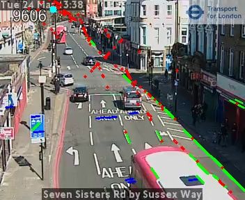
[5] Dong, R., Li, B., and Chen, Q.-m. An Automatic Calibration Method for PTZ Camera in
     Expressway Monitoring System. In 2009 WRI World Congress on Computer Science and
     Information Engineering, volume 6, pp. 636–640, March 2009. doi: 10.1109/CSIE.2009.763.
 [6] Dubska, M., Herout, A., and Sochor, J. Automatic Camera Calibration for Traffic Understanding.
     In Proceedings of the British Machine Vision Conference 2014, pp. 42.1–42.12, Nottingham,
     2014. British Machine Vision Association. ISBN 978-1-901725-52-0. doi: 10.5244/C.28.42.
     URL http://www.bmva.org/bmvc/2014/papers/paper013/index.html.
 [7] Faugeras, O. Three-dimensional computer vision: a geometric viewpoint. MIT Press, 1993.
 [8] Fung, G. S. K.       Camera calibration from road lane markings.    Optical En-
     gineering, 42(10):2967, October 2003.       ISSN 0091-3286.    doi:  10.1117/1.
     1606458.   URL http://opticalengineering.spiedigitallibrary.org/article.
     aspx?doi=10.1117/1.1606458.
 [9] HM Government. Open Government Licence, 2020. URL http://www.nationalarchives.
     gov.uk/doc/open-government-licence/version/3/.
[10] Lai, A. H. S., Yung, N. H. C., and Member, S. Lane detection by orientation and length
     discrimination. IEEE Trans. Syst., Man, Cybern. B, pp. 539–548, 2000.
[11] Liebowitz, D. and Zisserman, A. Metric rectification for perspective images of planes. In
     Proceedings. 1998 IEEE Computer Society Conference on Computer Vision and Pattern Recog-
     nition (Cat. No.98CB36231), pp. 482–488, June 1998. doi: 10.1109/CVPR.1998.698649. ISSN:
     1063-6919.
[12] Lin, T.-Y., Maire, M., Belongie, S., Hays, J., Perona, P., Ramanan, D., Dollár, P., and Zitnick,
     C. L. Microsoft COCO: Common Objects in Context. In Fleet, D., Pajdla, T., Schiele, B.,
     and Tuytelaars, T. (eds.), Computer Vision – ECCV 2014, Lecture Notes in Computer Science,
     pp. 740–755, Cham, 2014. Springer International Publishing. ISBN 978-3-319-10602-1. doi:
     10.1007/978-3-319-10602-1_48.
[13] Liu, W., Anguelov, D., Erhan, D., Szegedy, C., Reed, S., Fu, C.-Y., and Berg, A. C. Ssd: Single
     shot multibox detector, 2015.
[14] Luo, Z., Branchaud-Charron, F., Lemaire, C., Konrad, J., Li, S., Mishra, A., Achkar, A., Eichel,
     J., and Jodoin, P.-M. MIO-TCD: A New Benchmark Dataset for Vehicle Classification and
     Localization. IEEE Transactions on Image Processing, 27(10):5129–5141, October 2018. ISSN
     1941-0042. doi: 10.1109/TIP.2018.2848705. Conference Name: IEEE Transactions on Image
     Processing.
[15] Matters, T. f. L. |. E. J. Our open data, 2020. URL https://www.tfl.gov.uk/info-for/
     open-data-users/our-open-data.
[16] May, T. Lockdown-type measures look effective against covid-19. BMJ, 370, July 2020.
     ISSN 1756-1833. doi: 10.1136/bmj.m2809. URL https://www.bmj.com/content/370/
     bmj.m2809. Publisher: British Medical Journal Publishing Group Section: Editorial.
[17] Redmon, J. and Farhadi, A. Yolov3: An incremental improvement, 2018.
[18] Schoepflin, T. N. and Dailey, D. J. Dynamic camera calibration of roadside traffic management
     cameras for vehicle speed estimation. IEEE Transactions on Intelligent Transportation Systems,
     4(2):90–98, 2003.
[19] Schoepflin, T. N., Dailey, D. J., et al. Algorithms for estimating mean vehicle speed using
     uncalibrated traffic management cameras. Technical report, Washington (State). Dept. of
     Transportation, 2003.
[20] Sekachev, B., Manovich, N., Zhiltsov, M., Zhavoronkov, A., Kalinin, D., Hoff, B., TOsmanov,
     Kruchinin, D., Zankevich, A., DmitriySidnev, Markelov, M., Johannes222, Chenuet, M., a andre,
     telenachos, Melnikov, A., Kim, J., Ilouz, L., Glazov, N., Priya4607, Tehrani, R., Jeong, S.,
     Skubriev, V., Yonekura, S., vugia truong, zliang7, lizhming, and Truong, T. opencv/cvat: v1.1.0,
     August 2020. URL https://doi.org/10.5281/zenodo.4009388.

                                                 6
[21] Shapiro, L. and Stockman, G. Computer Vision. Prentice House London, 2001.
[22] Song, K.-T. and Tai, J.-C. Dynamic Calibration of Pan–Tilt–Zoom Cameras for Traffic Mon-
     itoring. IEEE Transactions on Systems, Man and Cybernetics, Part B (Cybernetics), 36(5):
     1091–1103, October 2006. ISSN 1083-4419. doi: 10.1109/TSMCB.2006.872271. URL
     http://ieeexplore.ieee.org/document/1703651/.
[23] Tsai, R. A versatile camera calibration technique for high-accuracy 3d machine vision metrology
     using off-the-shelf tv cameras and lenses. IEEE Journal on Robotics and Automation, 3(4):
     323–344, 1987.
[24] Zhang, Z., Tan, T., Huang, K., and Wang, Y. Practical Camera Calibration From Moving
     Objects for Traffic Scene Surveillance. IEEE Transactions on Circuits and Systems for Video
     Technology, 23(3):518–533, March 2013. ISSN 1558-2205. doi: 10.1109/TCSVT.2012.2210670.
     Conference Name: IEEE Transactions on Circuits and Systems for Video Technology.

                                                 7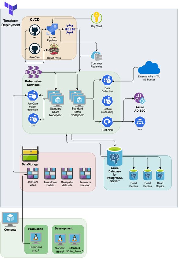
Appendix A   Deployment

                              Figure A.1: Project architecture.
                              Deployment provisioning is controlled
                              declaratively by Terraform, contain-
                              ing each component of the process-
                              ing pipeline. Kubernetes manages two
                              compute clusters: (1) A GPU acceler-
                              ated horizontally scaled video process-
                              ing pool; (2) A stability focused hori-
                              zontally scaled burstable CPU pool exe-
                              cuting scheduled tasks and hosting API
                              access points for direct data acquisition
                              and service for control centre output,
                              Figure A.2.

                              Figure A.2: Control centre output.
                              Provides real-time interactive pan-
                              London activity metrics in web applica-
                              tion format convenient to stakeholders.

                          8
Appendix B Intermediate Camera Planes
0
x-y plane
−120
50
−100
100
−80
1.02152annotatedimage-img0.png
150 −60
−40
200
−20
250
(u0, v0) = 313, −17 0
u1 = −2338
0 50 100 150 200 250 300 pixels −100 −75 −50 −25 0 25 50 75 metres
Figure B.1: Demonstration of perspective mapping of camera calibration from image to world
plane before estimated registration to British National Grid. Rays (black, solid) are drawn as grid
lines and extended (red, dashed) to the estimated vanishing points (u0 , v0 ) and (u1 , v0 ). When
mapped onto world coordinates. For example, vehicle trajectories (green, dotted) are mapped by this
transformation.
9You can also read