Monitoring Stream Temperatures- A Guide for Non-Specialists
←
→
Page content transcription
If your browser does not render page correctly, please read the page content below
Prepared in cooperation with the National Park Service

Monitoring Stream Temperatures—
A Guide for Non-Specialists
Chapter 25 of
Section A, Surface-Water Techniques
Book 3, Applications of Hydraulics

Techniques and Methods 3–A25

U.S. Department of the Interior
U.S. Geological Survey
Cover:
Upper left: East Pinnacles Creek looking north along The Pinnacles, Sierra National Forest, California.
Center: Sycan River looking upstream, Fremont National Forest, Oregon.
Lower right: Big Sawmill Creek looking upstream, Arc Dome Wilderness, Toiyabe National Forest, Nevada.
All photographs by Michael Heck, U.S. Geological Survey.
Monitoring Stream Temperatures—
A Guide for Non-Specialists
By Michael P. Heck, Luke D. Schultz, David Hockman-Wert, Eric C. Dinger, and
Jason B. Dunham

Chapter 25 of
Section A, Surface-Water Techniques
Book 3, Applications of Hydraulics

Prepared in cooperation with the National Park Service

Techniques and Methods 3–A25

U.S. Department of the Interior
U.S. Geological Survey
U.S. Department of the Interior
RYAN K. ZINKE, Secretary

U.S. Geological Survey
William H. Werkheiser, Deputy Director
   exercising the authority of the Director

U.S. Geological Survey, Reston, Virginia: 2018

For more information on the USGS—the Federal source for science about the Earth, its natural and living
resources, natural hazards, and the environment—visit https://www.usgs.gov or call 1–888–ASK–USGS.
For an overview of USGS information products, including maps, imagery, and publications,
visit https://store.usgs.gov.

Any use of trade, firm, or product names is for descriptive purposes only and does not imply endorsement by the
U.S. Government.

Although this information product, for the most part, is in the public domain, it also may contain copyrighted materials
as noted in the text. Permission to reproduce copyrighted items must be secured from the copyright owner.

Suggested citation:
Heck, M.P., Schultz, L.D., Hockman-Wert, D., Dinger, E.C., and Dunham, J.B., 2018, Monitoring stream
temperatures—A guide for non-specialists: U.S. Geological Survey Techniques and Methods, book 3, chap. A25,
76 p., https://doi.org/10.3133/tm3A25.

ISSN 2328-7055 (online)
iii

Contents

Executive Summary........................................................................................................................................1
Section 1. Getting Started—Why, What, Where, When?........................................................................1
Section 2. Standard Operating Procedures...............................................................................................8
Standard Operating Procedure (SOP) 1—Launching Data Loggers......................................................9
Standard Operating Procedure (SOP) 2—Calibration Check of Data Loggers..................................16
Standard Operating Procedure (SOP) 3—Installing Data Loggers in a Stream................................25
Standard Operating Procedure (SOP) 4—Downloading Data Loggers...............................................30
Standard Operating Procedure (SOP) 5—Offloading and Exporting Data in Hoboware Pro..........39
Standard Operating Procedure (SOP) 6—Importing and Managing Data..........................................47
Acknowledgments........................................................................................................................................63
References Cited..........................................................................................................................................63
Appendix 1. Data Logger Installation and Download Forms..............................................................67

Figure
        1.     Diagram showing standard operating procedure workflow..................................................8

Tables
        1. List of examples of how to describe elements of a thermal regime, including
           magnitude, variability, frequency, duration, and timing of temperatures............................3
        2. Categories of temperature descriptors and selected examples of associated biotic
           responses of stream biota to them.............................................................................................5
        3. Onset data loggers commonly used in stream temperature monitoring programs...........7
        4. Software and hardware components necessary to use Onset data loggers.....................7
iv

     Conversion Factors

     U.S. customary units to International System of Units

                    Multiply                       By                             To obtain
                                                  Length
     inch (in.)                                  2.54                 centimeter (cm)
     inch (in.)                                 25.4                  millimeter (mm)
                                                  Volume
     ounce, fluid (fl. oz)                        0.02957             liter (L)
                                                  Mass
     ounce, avoirdupois (oz)                    28.35                 gram (g)
     pound, avoirdupois (lb)                     0.4536               kilogram (kg)

     International System of Units to U.S. customary units

                    Multiply                       By                             To obtain
                                                  Length
     centimeter (cm)                              0.3937               inch (in.)
     millimeter (mm)                              0.03937              inch (in.)
     meter (m)                                    3.281                foot (ft)
     kilometer (km)                               0.6214               mile (mi)
     kilometer (km)                               0.5400               mile, nautical (nmi)
     meter (m)                                    1.094                yard (yd)

     Temperature in degrees Celsius (°C) may be converted to degrees Fahrenheit (°F) as follows:
     °F = (1.8 × °C) + 32.
Monitoring Stream Temperatures—A Guide for
Non-Specialists
By Michael P. Heck1, Luke D. Schultz1, David Hockman-Wert1, Eric C. Dinger2, and Jason B. Dunham1

Executive Summary                                                  and basic reporting. After reading through this protocol,
                                                                   non-specialists with an interest in monitoring streams and
      Water temperature influences most physical and               water quality will have the capability to effectively install
biological processes in streams, and along with streamflows        stream temperature data loggers to remotely record water
is a major driver of ecosystem processes. Collecting data          temperatures.
to measure water temperature is therefore imperative,
and relatively straightforward. Several protocols exist for        Why Monitor Water Temperature?
collecting stream temperature data, but these are frequently
directed towards specialists. This document was developed               In streams, temperature represents the collective influence
to address the need for a protocol intended for non-specialists    of many factors that influence heat exchanges (Caissie,
(non-aquatic) staff. It provides specific step-by-step             2006), including heat gains from solar radiation, inflows of
procedures on (1) how to launch data loggers, (2) check the        groundwater or tributaries, and losses of heat from evaporation
factory calibration of data loggers prior to field use, (3) how    or radiation to the atmosphere. Changes in streamflows,
to install data loggers in streams for year-round monitoring,      stream shading, and other factors can significantly influence
(4) how to download and retrieve data loggers from the field,      stream temperatures. Increasingly, changing precipitation
and (5) how to input project data into organizational databases.   patterns, decreasing snow cover and glaciers, and warming air
                                                                   temperatures, among other factors, have led to concerns about
                                                                   warming temperatures in streams (Isaak, Young, and others,
                                                                   2016). Collectively, temperatures in streams reflect all of these
Section 1. Getting Started—Why,                                    influences.
What, Where, When?                                                      Temperature also is a central force behind just about
                                                                   every biological process that takes place within stream
Is This Protocol for You?                                          ecosystems (Magnuson and others, 1979), ranging from the
                                                                   speed of chemical reactions to ecosystem productivity. Across
      Measuring stream temperature seems like a simple task,       the United States, altered stream temperatures are a leading
but in our experience the details matter. Accordingly, several     source of water quality impairment, leading to loss of cold
protocols are available for measuring stream temperatures          water for species like Pacific salmon (Oncorhynchus spp.) and
that provide guidelines to help avoid common pitfalls,             steelhead (Oncorhynchus mykiss; Poole and others, 2001) and
including Dunham and others (2005), Isaak and Horan (2011),        native trout from the west to east coast (Shepard and others,
Sowder and Steel (2013), U.S. Environmental Protection             2016). In short, simply measuring stream temperature can
Agency (2014), and Mauger and others (2015). Although              help us identify locations were restoration actions are needed,
thorough, these previous protocols lack the clear guidance for     provide us insight about how and why temperatures change
implementation for non-specialists. Our objective in this report   over time or vary in different locations, and help us anticipate
is to provide a simplified distillation of this advice for non-    the consequences of these changes for water quality and
specialists who may not have experience in monitoring stream       species distributions.
temperature, as well as providing standardized techniques

  1
      U.S. Geological Survey.
  2
      National Park Service.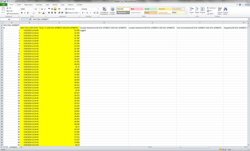
2   Monitoring Stream Temperatures—A Guide for Non-Specialists

Identifying the Key Questions about                                       exceeded thresholds that might cause biological stress
                                                                          for given fish species or other aquatic organisms.
Water Temperature
                                                                        • Duration refers to how long a given thermal condition
     The most important step in designing a temperature                   persists. For example, studies of cold-adapted stream
monitoring effort is to clearly identify the questions that               fish (such as trout) shows that thermal tolerance is a
information from monitoring will answer (Nichols and                      function of temperature (magnitude) and its persistence
Williams, 2006). Common research questions regarding water                (duration, expressed as the number of days that
temperature include the following:                                        temperatures exceed a critical threshold; Wehrly and
    • How are temperatures in streams changing over time?                 others, 2007).
      This could be related to an interest in daily fluctuations
      in temperature, the seasonality of temperature or                 • Timing of temperatures also is important because it
      thermal regimes, or changes across years or longer                  may influence the onset of different portions of the life
      periods of time—up to 30 years or longer in the case of             cycle of aquatic organisms (for example, spawning,
      tracking climate-related changes.                                   hatching, migration) or seasonality of factors with
                                                                          major ecosystem consequences (such as onset of algal
    • How do temperatures relate to potential causes of                   blooms). Biologists often apply the term phenology
      heating or cooling? This could be related to the                    to the timing of biological events, such as hatching,
      importance of changes to shading of streams from                    flowering, or many other types of responses, and there
      solar radiation, influences of heat exchanges with                  are well established broad phenology networks to track
      groundwater, lakes, or runoff from glaciers and                     these events in response to changes in weather and
      snowfields, or an interest in how stream temperatures               climate (USA National Phenology Network accessed at
      track air temperatures.                                             https://usanpn.org/).
    • How do stream biota respond to temperature? This                  Collectively, variation in temperature across seasons
      could involve relating temperature to the presence,          within a year, and among years, can be defined as a thermal
      abundance, or growth of species. Summaries of                regime, which can be defined in terms of magnitude,
      temperature such as magnitude, variability, frequency,       variability, frequency, duration, and timing of temperatures
      duration, and timing could drive biotic processes.           (Arismendi and others, 2013a; Maheu and others, 2015;
                                                                   table 1).
     The following sections provide guidance on how to frame            For practical purposes, the many ways in which status
specific questions of interest for any monitoring effort.          can be described indicate that it is critical to be clear on what
     Status.—The simplest question that can be asked about         aspects of thermal regimes are of most interest. Furthermore,
temperature is “what is it?” This relates to the status of         by embracing a regime-based view of temperature, one can
temperature in a location and time sampled within a given          gain a tremendous range of useful insights (Arismendi and
stream. As with many aspects of temperature, status can have       others, 2013a), just as can be done for air temperatures. For
many meanings.                                                     example, for the purpose of water-quality criteria, thermal
     Because temperature is a continuous phenomenon, status        regimes are often considered in the context of only a single
can refer to many characteristics. Variation in temperature        weekly summary of maximum temperatures (McCullough,
over time can be framed in terms of the magnitude, frequency,      2010). The other 358 days of a typical year also have value
duration, and timing of events (Arismendi and others, 2013a).      in describing stream temperature status; one should consider
    • Magnitude simply refers to how warm or cold                  the costs and benefits of seasonal compared to year-round
      temperatures are. Understanding magnitude can                sampling in this context. Few terrestrial ecologists would
      be important for addressing questions about water            consider data from a single week sufficient in describing a
      quality, for example, where water-quality criteria are       thermal regime.
      often specified in terms of magnitudes (Falke and                 Trends.—Changes in status over time are often
      others, 2016).                                               referred to as trends. A common meaning of trend refers to
                                                                   a progressive change over time, such as a simple pattern of
    • Variability refers to temporal fluctuations in               warming or cooling that may happen in a stream. Other more
      temperature across a given time period. Although             complex patterns of change are possible, such as temperature
      stream fishes have adapted to withstand temperatures         cycles linked to climate. Trends can be considered on any time
      fluctuating on a daily basis, the magnitude of that          scale. Variation among hours within a day may be of interest
      fluctuation must remain within their range of biological     to understand short-term exposures of species to temperature
      tolerances.                                                  (McCullough, 2010). Seasonal warming and cooling (variation
    • Frequency refers to how many times a given thermal           among days within a season) is another common response of
      condition is observed. For example, there may be             interest. Annual trends in temperature can provide important
      an interest in how many times water temperatures             clues about responses to short-term events such as wildfires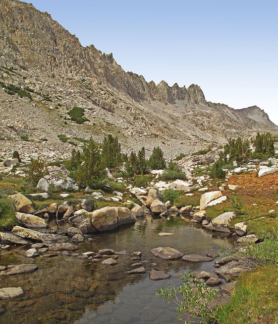
Section 1. Getting Started—Why, What, Where, When?   3

             Table 1. List of examples of how to describe elements of a thermal regime, including magnitude,
             variability, frequency, duration, and timing of temperatures.
             [Modified from Benjamin and others (2016). Descriptor: The values in the table below (16, 18, and 20 °C) are common
             thresholds for mean or maximum temperatures associated with tolerances of coldwater species (cooler values are applied to
             some species or sensitive life stages [McCullough, 2010]). CTD, Cumulative Temperature Distribution is the date when each
             site reached the 50th or 75th percentile of total degree days. Abbreviations: n, number (quantity of); °C, degrees Celsius;
             >, greater than; %, percent]

                    Category             Descriptor                                            Definition
              Magnitude (°C) Maximum                         Warmest temperature (typically of the year)
                             MWMT                            Maximum Weekly Maximum Temperature1
                             MWAT                            Maximum Weekly Average Temperature2
                             Degree days                     Accumulation of temperatures over time3
              Variability (°C)    Mean range                 Difference between the highest and lowest daily mean
                                  Max range                  Difference between the highest and lowest maximum
                                  Mean variance              A statistical measure of deviations among daily means
                                  Max variance               A statistical measure of deviations among daily maximums
              Frequency (n)       Days > 16 °C               Number of days in the record that exceeded 16 °C
                                  Days > 18 °C               Number of days in the record that exceeded 18 °C
                                  Days > 20 °C               Number of days in the record that exceeded 20 °C
              Duration (n)        Consec. days > 16 °C       Consecutive number of days in the record that exceeded 16 °C
                                  Consec. days > 18 °C       Consecutive number of days in the record that exceeded 18 °C
                                  Consec. days > 20 °C       Consecutive number of days in the record that exceeded 20 °C
              Timing              CTD 50%                    Date of attaining 50% of the degree days in a given time frame4
                                  CTD 75%                    Same as above, but for 75% of the distribution
                1
                 Highest 7-day average of maximum daily temperatures in any season or year.
                2
                 Highest 7-day average of average daily temperatures in any season or year.
                3
                 Can be calculated by adding up average temperature for each day greater than zero degrees.
                Summing degree days provides a tally of cumulative temperatures. Fifty percent is the point at which one-half of the total
                4

             heat has accumulated within a time frame (for example, within a year).

(Dunham and others, 2007; Heck, 2007) or longer-term                          (Isaak, Wenger, and others, 2016), and have been used to
changes in climate (Isaak, Young, and others, 2016). As of this               understand the distributions of temperature-sensitive species in
writing, however, there are surprisingly few streams that have                streams.
been monitored for long-enough times (>10 years) to detect                          Additionally, stream temperatures can vary at extremely
reliable trends in the face of regionally changing climates                   fine spatial scales, sometimes with biologically significant
(Isaak and others, 2012; Arismendi and others, 2014; Luce and                 influences at scales of 1 m or less in the case of coldwater
others, 2014).                                                                thermal refuges (Torgersen and others, 2012). In short, one can
      Spatial variation.—In recent years, a host of new spatial               think of spatial variation in terms of the extent of the system
statistical models have emerged that provide powerful new                     of interest and the resolution, or grain, at which information
capabilities for modeling patterns of temperature in whole                    is sought (Peterson and Dunham, 2010). Examples of extent
stream networks (Falke and others, 2013; Ver Hoef and others,                 include questions about a watershed or stream network, or
2014; Isaak and others, 2014; McNyset and others, 2015).                      perhaps questions within the boundaries of a given jurisdiction
In practical terms, this means that it is possible to efficiently             (for example, a National Park or National Forest, State, or
make connections among locations sampled for stream                           other category of land ownership), and not tied to a specific
temperatures to provide a robust and continuous model-based                   watershed. Within a given spatial extent, one can monitor
prediction of stream temperatures. The more points that are                   temperature at a given resolution (for example, samples every
sampled and how they represent variation in a stream network                  1 km, every 100 m, and so on) to produce a representation
result in more accurate and precise predictions at non-sampled                of how stream temperatures change through space (Fullerton
locations (Som and others, 2014). For example, based on                       and others, 2015). The same analogy regarding scale here also
existing data, maps of stream temperatures derived from these                 applies to time, which we discussed previously in section,
new models have been produced for much of the Northeastern                    “Trends” (Steel and Lange, 2007; Peterson and Dunham, 2010).
(DeWeber and Wagner, 2015) and Western United States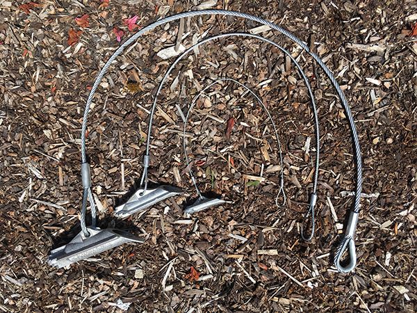
4   Monitoring Stream Temperatures—A Guide for Non-Specialists

      Factors influencing temperature.—In our coverage                   • Changes in snow and ice cover, rainfall, and
of questions related to status, trends, and spatial variation,             streamflows. Melting snow and ice can lead to
we have already indicated some examples of questions tied                  substantial cooling of streams, and in combination
to understanding factors that influence stream temperature.                with rainfall contribute to greater streamflows. Larger
Ideally, one would quantify each component of the heat budget              streams take more energy to heat. Understanding
of a stream and be able to use the basic laws of physics to                sources of water, and how they are delivered over time
understand stream temperature. If there is an interest in factors          (for example, seasonal patterns of rain, snow, or ice
that influence stream temperature, it is important to consider             melt), in combination with how water moves through
how streams heat in the context of a heat budget (Caissie,                 the landscape into streams (for example, storage in
2006), the linkages between these factors and natural or                   aquifers), can be important to understanding heating of
human influences on temperature (Poole and Berman, 2001),                  streams.
and what kinds of information are available that could serve
as useful indicators of these influences (for example, geology,          • Changes in the shape of the stream channel. The
landform, climate, or vegetation; Wigington and others,                    complexity of stream channels, particularly in cases
2012). Boyd and Kasper (2003) provide a useful, detailed                   of complex floodplains or wetlands, can result in
review of specific factors that influence heating of streams,              increased complexity of stream temperatures. This
including factors influencing shade (for example, topographic              can provide species that can move an opportunity to
and streamside vegetation), heat transfers from below-                     take advantage of cold or warm spots in these places
surface waters or mixing with tributaries, air temperatures,               to better meet their thermal requirements to complete
evaporation, and streamflows.                                              their life cycles. Localized inputs of groundwater or
      In practice, complete accounting for the heat budget of              inputs of solar energy (for example, from lakes or
streams is seldom possible (Caissie, 2006). An alternative                 ponds) are common examples of factors influencing
approach to understanding factors that influence stream                    temperatures in these settings.
temperature is through structured experimental manipulations             • Changes in below-surface waters. Changes in
(Johnson and Jones, 2000; Groom and others, 2011), but these               availability or temperature of groundwater or how
can be expensive and difficult to implement, particularly                  water moves between the surface and sub-surface
in areas where strong land- and water-use restrictions are                 within streams (through changes in shape of the stream
in effect. It is also difficult to conduct these experiments at            channel) can affect stream temperatures (that is,
scales that are relevant to management concerns about stream               relatively constant temperatures of spring-dominated
temperature (Fausch and others, 2002). Consequently, much of               streams compared to streams dominated by runoff and
our understanding of factors that influence stream temperature             shallow groundwater storage).
relies on observational and correlational approaches (Caissie,
2006). For example, Isaak, Ver Hoef, and others (2016)                   • Influences of lakes or reservoirs. Water at the surface
and Falke and others (2015) used spatial statistical models                of lakes and reservoirs spends more time in the sun and
to explore linkages between recent wildfires and spatial                   can contribute heat to streams the surface water flows
variability of temperatures in stream networks.                            into. If water is released from the bottom of a deep
      Examples of factors that are commonly studied in relation            reservoir into a stream, however, temperatures may be
to changes in stream temperature include the following (see                cooled in warmer seasons of the year. Many reservoirs
Caissie [2006] for further detail):                                        are seasonally stratified into a warm top layer and cold
     • Changes in stream-side vegetation or shading. Trees,                bottom layer in summer.
       shrubs, and other vegetation along the banks of                   • Climate change. All influences on stream temperature
       streams, and in some cases (such as very tall trees) in             previously listed are directly or indirectly related to
       upland areas, can intercept sunlight and prevent solar              the known and potential influences of climate change.
       radiation from reaching water in the stream channel.                For example, a recent drought in the Western United
       Changes in vegetation occur seasonally (such as loss of             States led to losses of vegetation (from wildfire), low
       leaves in fall or leaf-out in spring) and annually (such            streamflows, and increased water temperatures in a
       as forest growth, tree mortality, or changes in the types           large stream network (Schultz and others, 2017).
       of vegetation) in response to many different natural
       and human influences. Shading is more likely to have              In practice, at least some of the factors listed here are
       an effect on smaller streams.                                likely to play into questions about stream temperature to be
                                                                    addressed through monitoring.
Section 1. Getting Started—Why, What, Where, When? 5
Implications for biota.—Water temperature and Sampling Design
streamflow are considered to be the two most influential
variables that control stream biota and ecosystems (Magnuson After monitoring questions are identified, the next step
and others, 1979; Poff, 1997). In practice, stream temperatures is to consider a sampling design. In short, a sampling design
and flows often fluctuate together, with interactive effects considers both the population of interest or sampling frame
on biota (Arismendi and others, 2013b; Kovach and others, and how it is sampled. The population of interest consists
2015). Accordingly, many questions about stream temperature of all of the possible observations within a defined frame
are focused on its effects on biota. To protect temperature- of inference, for example, all of the possible locations that
sensitive species, many states have identified biological could be instrumented within a given water body. It is usually
temperature criteria for Clean Water Act regulation (see Todd impossible or impractical to survey everything; a subset or
and others [2008]) or developed methods to integrate spatial sample of the population is often drawn to make an inference
models of stream temperature with biological criteria to about the population as a whole. The manner in which a
diagnose thermal impairment of streams (Falke and others, sample is drawn influences the bias and precision of the
2016). In short, when considering questions about biota, inferences about a population—how well a sample represents
consider which species are in question (fish, amphibians, the population. Bias is the degree to which a sample truly
macroinvertebrates, and so on), and how they are hypothesized represents the population, and precision refers to how strongly
to respond to temperature (survival, growth, and phenology). inferences about a population are resolved. A robust sampling
There are an extensive amount of examples of studies relating design should consider the need to control both bias and
individual species to different measures of stream temperature; precision.
we provide a few examples here to illustrate a range of A full treatment of sampling design is outside of the
possibilities (table 2). purview of this protocol, and decisions and intricacies of
It is not possible here to cover all considerations involved sample design should not sway or deter an individual from
in addressing questions about biota (or ecosystem effects of collecting temperature data. The background presented here
stream temperature), except to emphasize that these questions is intended to provide a reference for those with an interest in
are best served by engaging individuals with specialized the basics of sample design considerations. Given the scarcity
expertise from the start of a monitoring effort. of long-term, year-round temperature data, any information
Table 2. Categories of temperature descriptors and selected examples of associated biotic responses of stream biota to them.
[Category: n, number; °C, degrees Celsius]
Category Descriptor Examples of biotic responses
Magnitude (°C) Maximum and minimum Short-duration or acute physiological stress or death if temperatures are too warm (for example,
temperatures trout and salmon; McCullough, 2010) or too cold (for example, smallmouth bass; Horning
and Pearson, 1973).
Degree days Indicator of development time or growth potential in fish (Neuheimer and Taggart, 2007)
and stream insects (Everall and others, 2015). Degree days includes both a description of
magnitude and duration of exposure.
Variability (°C) Temporal variance Increased variability in temperatures may lead to greater likelihood of physiological stress in a
location (Kammerer and Heppell, 2013).
Spatial variation Species need to invest more effort in finding suitable temperatures among locations within a
network of streams when spatial variation in thermal suitability increases (Torgersen and
others, 2012).
Frequency (n) Days Number of days in the record that exceed critical thresholds explained the distribution of
different species of native and nonnative trout (Benjamin and others, 2016).
Timing Date Species may be adapted to the specific timing of temperatures in systems to successfully
complete their life cycles (Vannote and Sweeney, 1980).6 Monitoring Stream Temperatures—A Guide for Non-Specialists
gained will be useful for many purposes. At a minimum, we ease of access, safety concerns, or other concerns not related
recommend documenting the decision process for (1) where to statistical representation. However, subjective samples
and when samples were collected, (2) the frequency of cannot be thought to faithfully represent a larger population
sampling, (3) total number of samples, and (4) method of of possible samples within a population or sampling frame.
sample allocation. We discuss each of these points briefly here The other end of the continuum is a purely random or equal
to help the non-specialist enter into discussions with sampling probability sample. This means that each possible location
experts. in space or time has an equal chance of being sampled.
Where and when to sample.—The answer to this Probabilistic samples such as this provide a much more
question depends on the monitoring objectives. If the reliable representation of the population or sampling frame.
objective is to understand the seasonal fluctuations at a There are many other examples of probabilistic designs (Som
previously monitored site, then the answer is simple: deploy and others, 2014).
the data logger at the previously monitored site for a full-year
deployment to represent all seasons. Multi-year deployments
also may be of interest, particularly if climate-related A Few Preliminary Notes
associations are relevant (where 30 years or more of data are
Because this guide is written for non-specialists, we
most desirable). If the monitoring objective is to quantify
assume users are working with limited resources and hoping to
the distribution of thermal regimes in a given area, then the
accomplish useful temperature monitoring to address a limited
placement requires more thought. Examples include patterns
scope of objectives or questions about stream temperature.
of temperature among possible locations to sample within a
Virtually any collection of high-quality stream temperature
given land ownership, range of a species of concern, water
data can be tremendously useful. For example, crowdsourcing
body (lake or stream network), water body type (perennial or
of temperature data from a variety of local monitoring
intermittent), or any other possible frame of inference.
efforts has long been the source of valuable temperature
Frequency of sampling.—Frequency of sampling
information on a national (Eaton and others, 1995) and
refers to how often temperatures are recorded. Given the high
regional basis (Dunham and others, 2003; DeWeber and others,
memory capacity of temperature data loggers, an interval of at
2015; Chandler and others, 2016). Thus, even collection
least 1 hour or less is a good rule of thumb. Longer intervals
of temperature data from a single location to address local
between measurements run the risk of missing important high
objectives has potential to contribute significant information
or low temperatures within a day (Dunham and others, 2005).
for regional to national applications.
Sample size.—Desirable sample sizes, or number
Before getting into the details of how to monitor stream
of locations sampled, depend on the size or extent of the
temperature, a few preliminary considerations should be taken
sampling frame and specific objectives of the sampling effort,
into account: (1) the identification of relevant safety protocols,
and the degree of variability in temperatures among sites.
(2) the selection of temperature data loggers and data storage
Temperatures can vary over very small (30), even
bodies of water. Beyond that, we encourage all users to consult
for smaller sampling frames. Note that any temperature data
safety officers within their local units or other experienced
collection can be valuable, even if available resources limit
personnel for specific guidance on this topic.
sample sizes.
Sample allocation.—Sample allocation refers to
how samples are distributed in space or time. The simplest
approach is to distribute samples subjectively, based onSection 1. Getting Started—Why, What, Where, When? 7
In regard to selection of temperature data loggers prior to stepping foot in a stream is paramount to a safe and
a variety of options are available (Dunham and others, successful monitoring project. Installations should take place
2005; U.S. Environmental Protection Agency, 2014). For at base flow to ensure loggers can be placed safely in the
consistency, we focus on a single brand of instruments thalweg. The thalweg is defined as the deepest part of the
(table 3) and their associated hardware and software (table 4). channel at any given cross section. Installing a data logger
Further, we focus on a single data storage software package during high flows is not only dangerous to field personnel but
(see SOP 6—Importing and Managing Data) so we can be can lead to failure to place the data logger in a deep enough
specific on protocols to use. That said, the protocols described location to stay wet as streamflows recede (unless the entire
here can be adapted to a wide variety of temperature data channel dries). Additionally, if interested in year-round
loggers and software packages. The basic concepts of monitoring, additional considerations as to placement location
launching, checking the calibration, installing in a stream, would be required given the higher probability of loss or
downloading, and exporting of data are all necessary damage to equipment and thereby data. A review of historical
components of any monitoring project. data from U.S. Geological Survey streamgages (https://
The timing of field operations will have a profound waterdata.usgs.gov/usa/nwis/rt) can be useful for anticipating
influence on data quality as well as the safety of the field when suitable low flows are likely to occur on a particular
personnel. Becoming familiar with a hydrologic regime stream or within a given watershed.
Table 3. Onset data loggers commonly used in stream temperature monitoring programs.
[Accuracy: Accuracy for commonly observed stream temperatures (0–35 °C). Unit cost: $, U.S. dollars. Abbreviations: cm, centimeter; m, meter ; °C, degrees
Celsius]
Battery
Accuracy Resolution Replaceable Memory Waterproof Dimensions Unit
Data logger life
(°C) (at 25 °C) battery? (measurements) (m) (cm) cost
(years)
Onset HOBO® Water Temperature Pro v2 ±0.21 0.02 °C 6 No 42,000 to 120 m 3.0 × 11.4 $129
U22-001
Onset HOBO® 64K Pendant® Temperature ±0.53 0.14 °C 1 Yes 52,000 to 30 m 5.8 × 3.3 × 2.3 $59
UA-001-64
Onset HOBO® TidbiT® v2 ±0.21 0.02 °C 5 No 42,000 to 305 m 3.0 × 4.1 × 1.7 $133
UTBI-001
Table 4. Software and hardware components necessary to use Onset® data loggers.
[Unit cost: $, U.S. dollars]
Product Purpose Unit cost
Onset HOBOware Pro Software
®
Software used for all HOBO data loggers. Use software to launch and read out data
®
$99
BHW-PRO-DLD loggers, plot data, and export for further analysis.
Onset Optic USB Base Station Hardware interface between Onset® data loggers and HOBOware® Pro. Use the base station $124
BASE-U-4 to launch the loggers on a PC/Mac. Couplers are included for compatibility with Onset
U22, Pendant®, and TidbiT® data loggers.
Onset HOBO® Waterproof Shuttle Use the waterproof shuttle to download and re-launch the loggers in the field. Connect the $249
U-DTW-1 waterproof shuttle to a PC/Mac to offload that data into HOBOware® Pro. Waterproof
to 20 meters. Couplers are included for compatibility with Onset U22, Pendant®, and
TidbiT® loggers.8 Monitoring Stream Temperatures—A Guide for Non-Specialists
Section 2. Standard Operating Procedures
Introduction
Figure 1 shows the workflow of the standard operating procedures. Please note that these procedures refer primarily to
Onset data loggers. These are commonly used products with which we are most familiar, but procedures for other products
would be similar.
Launching Data Loggers
How to program data loggers to record data at a specific interval using proprietary software
Calibration Check of Data Loggers
How determine if data loggers are measuring temperature to the manufacturer's specifications
Installing Data Loggers in a Stream
How to anchor a data logger in a stream channel for year-round data collection
Downloading Data Loggers
How to download data and re-launch a data logger in the field using a waterproof shuttle
Offloading and Exporting Data in HOBOware Pro
How to offload data from a waterproof shuttle and export those data from HOBOware Pro
Importing and Managing Data
How to import data into a database, such as Aquarius Time-Series software
Figure 1. Diagram showing standard operating procedure workflow.Standard Operating Procedure (SOP) 1—Launching Data Loggers 9
Standard Operating Procedure (SOP) 1—Launching Data Loggers
Overview
This SOP describes how to program temperature data loggers prior to a calibration check or installation in the field. This
SOP covers setting a logging interval, programming a delayed launch, and which metrics to record.
Supplies
• Computer with HOBOware Pro software installed
• Onset Optic USB Base Station
• Onset data loggers (U22, Pendant, or TidbiT)
• COUPLER2-A (for Pendant), COUPLER2-C (for U22), or COUPLER2-D (for TidbiT)
Procedure—Set Up HOBOware Pro Software c. Select SI from Unit System drop-down, then click
Next (fig. 1.3)
1. Install HOBOware Pro. d. Leave all Data Assistants boxes checked, then click
2. Open HOBOware Pro and continue through the Next (fig. 1.4)
HOBOware Setup Assistant.
a. Click Start (fig. 1.1)
b. Click USB devices only > Next (fig. 1.2)
Figure 1.3. Screen capture showing HOBOware Setup Assistant
Unit System dialog box.
Figure 1.1. Screen capture showing HOBOware Pro initial Setup
Assistant dialog box.
Figure 1.2. Screen capture showing HOBOware Setup Assistant Figure 1.4. Screen capture showing HOBOware Setup Assistant
Device Types selection dialog box. Data Assistants selection dialog box.®
10 Monitoring Stream Temperatures—A Guide for Non-Specialists
e. Select whether or not to send metrics to Onset b. In the navigation pane, click Display, then click
Computer Corporation, then click Next (fig. 1.5). Series to access options (fig. 1.8).
f. Click Done (fig. 1.6) c. Check the box next to Show the option to log
battery, then click OK.
3. Select the option to log battery voltage.
4. Complete steps 1–3 only once as these settings will
a. On main screen, click File > Preferences (fig. 1.7). remain until an update is installed. After updates are
installed, repeat steps 1–3.
Figure 1.5. Screen capture showing HOBOware Setup Assistant Figure 1.6. Screen capture showing HOBOware Setup Assistant
Help improve HOBOware? dialog box. Congratulations… dialog box.
Figure 1.7. Screen capture showing HOBOware Pro Preferences… option under the File menu.Standard Operating Procedure (SOP) 1—Launching Data Loggers 11
Figure 1.8. Screen capture showing HOBOware Pro Preferences dialog box, Display tab and Series preferences.
Procedure—Launch a Data Logger b. Wait a few seconds for the data logger to be detected
by the computer. If no data logger is detected, check
1. Connect the Onset Optic USB Base Station to the all connections, especially the data logger/coupler
computer using the USB cable and the temperature data connection, and make sure the data logger is fully
logger to the base station using the appropriate coupler inserted.
(fig. 1.9). c. For older versions of U22 data loggers, make sure
a. Data loggers can occasionally have a tight fit with the arrow printed on the outside of the data logger is
the coupler. A data logger is fully inserted when you lined up with the arrow on the coupler.
hear an audible “click.” d. For newer versions of U22 data loggers, a ridge on
the optic end should match the groove in the coupler,
ensuring good alignment.
Figure 1.9. Photograph showing Onset couplers for Onset data loggers. From
left to right: Coupler2-A for Pendant data loggers, Coupler2-C for U22 data
loggers, and Coupler2-D for TidbiT data loggers.12 Monitoring Stream Temperatures—A Guide for Non-Specialists
2. On the main screen, click Device > Launch… to open 4. Record the unique data logger serial number from the
the Launch Logger dialog box (fig. 1.10). Launch Logger dialog box (fig. 1.12).
3. Create a Launch Worksheet to record basic metrics from 5. In the Sensors group box, make sure both Temperature
the launch process (fig. 1.11). Only use the Launch and Logger’s Battery Voltage boxes are checked
Worksheet for field installations (SOP 3—Installing Data (fig. 1.13).
Loggers in a Stream). There is no need to record basic
metrics from a calibration check (SOP 2—Calibration
Check of Data Loggers).
Figure 1.10. Screen capture showing HOBOware Pro Launch… option under the Device menu.
Serial# LaunchDate LaunchTime LaunchVoltage Interval
10950791 6/13/2016 8:00am 3.48 1 hour
Figure 1.11. Example of a Launch Worksheet.Standard Operating Procedure (SOP) 1—Launching Data Loggers 13 Figure 1.12. Screen capture showing HOBOware Pro Launch Logger dialog box. The red oval highlights the unique data logger serial number. Figure 1.13. Screen capture showing HOBOware Pro Launch Logger dialog box. The red oval highlights Temperature and Logger’s Battery Voltage check boxes.
14   Monitoring Stream Temperatures—A Guide for Non-Specialists

 6.   In the Deployment group box, select desired logging                b.   Record the date/time of the delayed start on the
      interval from the Logging Interval drop-down list                       Launch Worksheet (fig. 1.11).
      (fig. 1.14).
                                                                    8.   Click Delayed Start to launch the data logger.
      a.   Logging interval recommendations are: 10 seconds
           for calibration checks (SOP 2—Calibration Check          9.   Record the battery voltage at the time of launch on the
           of Data Loggers) and 1 hour for field installations           Launch Worksheet. Voltage is important to note because
           (SOP 3—Installing Data Loggers in a Stream). A                installing a data logger with a low battery could result in
           1-hour logging interval has been shown to have                data loss.
           a low probability of missing the daily maximum                a.   On main screen, click Device > Status (fig. 1.15).
           temperature by more than 1°C (Dunham and others,
           2005, fig. 5).                                                b.   The battery voltage is shown in the Current
                                                                              Readings group box of the Status dialog box
 7.   In the Deployment group box, select a delayed start in                  (fig. 1.16).
      Start Logging: On Date/Time and set to mm/dd/yy at
      hh:mm:ss. This is the time when the data loggers will              c.   Onset U22 data logger battery voltage should be
      activate and begin recording temperatures.                              greater than 3.3 volts (V); and Onset TidbiT and
                                                                              Onset Pendant data loggers battery voltage should be
      a.   A delayed start will reduce, but not eliminate, the                greater than 2.7 V. Send data loggers with voltages
           amount of measurements collected before the data                   below these levels back to the manufacturer.
           logger is installed in a stream. It is acceptable for
           data loggers to begin recording several days or         10.   Disconnect the data logger from the base station. It is
           weeks before their field installation as long as data         now ready for its calibration check (SOP 2—Calibration
           recorded prior to installation is flagged as “pre-            Check of Data Loggers) or installation in the field
           install” at the conclusion of monitoring.                     (SOP 3—Installing Data Loggers in a Stream).

                         Figure 1.14. Screen capture showing HOBOware Pro Launch Logger dialog box. The
                         red oval highlights the Logging Interval drop-down list.
Standard Operating Procedure (SOP) 1—Launching Data Loggers 15
Figure 1.15. Screen capture showing HOBOware Pro Status… option under the Device menu.
Figure 1.16. Screen capture showing HOBOware Pro Status dialog box.16 Monitoring Stream Temperatures—A Guide for Non-Specialists
Standard Operating Procedure (SOP) 2—Calibration Check of Data Loggers
Overview
This SOP describes how to determine if data loggers are measuring temperature to the manufacturer’s specifications.
Thermometers and data loggers calibrated to National Institute of Standards and Technology (NIST) standards are available
as a reference during calibration checks. A calibration check should be performed before and after each field installation.
A calibration check consists of data loggers recording for 30 minutes in a warm bath, 30 minutes in a cool-down bath, and
30 minutes in a cold bath. This process takes approximately 2 days to complete.
Supplies
• Three coolers (large enough to submerge all data loggers with lots of extra room)
• Crushed ice
• Onset data loggers (U22, Pendant, or TidbiT)
• One NIST-calibrated Onset data logger (use same model as data logger being calibrated: U22, Pendant, or TidbiT)
• 8-in. cable/zip ties (0.095 in. width)
• 10-oz lead fishing weights (one weight per five data loggers)
• Onset Optic USB Base Station
• COUPLER2-A (for Pendant), COUPLER2-C (for U22), or COUPLER2-D (for TidbiT)
• Computer with HOBOware Pro software installed
Procedure—Day 1 b. Set a delayed start to a time the following day to
initiate the calibration check. Make sure there is
1. Fill a cooler about 3/4 full with room temperature adequate time to set up the cold bath (see step 4).
water and place in a climate controlled room (stable air c. Create a Calibration Check Worksheet to record
temperature). This will be the warm bath. basic metrics from the calibration process (fig. 2.1).
2. Launch data loggers, including the NIST-calibrated data d. Record the serial number and battery voltage at the
logger following procedures in SOP 1. time of launch on Calibration Check Worksheet.
a. Select a 10 second logging interval.
Serial# CalibVoltage CalibDate CalibMeanWarmDiff CalibMeanCoolDiff
10768077 3.57 7/26/2016 0.068 0.011
10768078 3.54 7/26/2016 0.057 0.084
10768079 3.57 7/26/2016 0.019 0.000
10768080 3.57 7/26/2016 0.043 0.055
Figure 2.1. Example of a Calibration Check Worksheet.Standard Operating Procedure (SOP) 2—Calibration Check of Data Loggers 17
3. Bundle five data loggers and one 10-oz lead fishing Procedure—Day 2
weight together with an 8-in. cable/zip tie (fig. 2.2).
4. Immerse launched and bundled data loggers in the warm 1. Approximately 3 hours before the data loggers are
bath and let soak overnight with the cooler lid open programmed to start recording, fill two coolers about 3/4
(fig. 2.3). full with crushed ice and add cold water until ice is fully
immersed in water.
a. Close lids and place coolers in the same climate
controlled room (stable air temperature). These will
be the cool-down and cold baths.
2. Following the delayed start time, begin mixing the water
in the warm bath by gently lifting one end of the cooler
about 4 in. off the ground.
a. Repeat this mixing/lifting about every 20 seconds for
30 minutes. The warm calibration check is complete.
3. Remove the bundled data loggers from the warm bath
and immerse them in the cool-down bath (one of the two
coolers with ice/water mixture) and close the lid.
a. The cool-down bath is used to decrease the
temperature of the data loggers from room
temperature to about 0 °C.
b. Leave the data loggers in the cool-down bath for
30 minutes.
4. Remove the bundled data loggers from the cool-down
bath and immerse them in the cold bath.
5. Mix the water in the cold bath by gently lifting one end
of the cooler about 4 in. off the ground.
a. Repeat this mixing/lifting about every 20 seconds for
Figure 2.2. Photograph showing five Onset U22 data loggers 30 minutes. The cold calibration check is complete.
attached to a 10-ounce lead weight with an 8-inch cable/zip
tie. 6. Open HOBOware Pro software and download all the
available updates, if prompted (fig. 2.4)
7. Connect the Onset Optic USB base station to
the computer using the USB cable and connect a
temperature data logger to the base station using the
appropriate coupler (see SOP 1—Launching Data
Loggers).
Figure 2.3. Photograph showing four clusters of five
Onset U22 data loggers soaking in a warm bath used for a Figure 2.4. Screen capture showing HOBOware Pro Check for
calibration check. Updates? dialog box.18 Monitoring Stream Temperatures—A Guide for Non-Specialists
8. Readout data from the data logger. c. Create or select a folder in which to store .hobo file,
then save the file (fig. 2.7).
a. On the HOBOware Pro main screen, click Device >
Readout… (fig. 2.5). d. The Plot Setup dialog box will open (fig. 2.8). To
see a graph of the data, click Plot, otherwise click
b. When prompted to stop the data logger, click Stop Cancel.
(fig. 2.6).
Figure 2.5. Screen capture showing HOBOware Pro screen capture showing the Readout… option under the Device menu.
Figure 2.6. Screen capture showing HOBOware Pro Stop
Logger? dialog.Standard Operating Procedure (SOP) 2—Calibration Check of Data Loggers 19
Figure 2.7. Screen capture showing HOBOware Pro Save dialog box to determine the
location to save a .hobo file.
Figure 2.8. Screen capture showing
HOBOware Pro Plot Setup dialog box.20 Monitoring Stream Temperatures—A Guide for Non-Specialists
9. Disconnect the temperature data logger from the base b. Browse to the folder where the .hobo files were
station. After readout, the data logger will be stopped saved and select all the files, then click Continue
and will remain in that state until it is launched again. (fig. 2.10).
10. Continue to readout data from all data loggers (repeat c. In the Choose Export Folder dialog box, choose
step 7). folder where to save the .csv files, then click Export
(fig. 2.11).
11. After reading out data from all data loggers, export the
.hobo files as .csv files. d. When the bulk file export is complete, click OK.
a. On the HOBOware Pro main screen, click 12. Close HOBOware Pro.
Tools > Bulk File Export > Select Files to
Export… (fig. 2.9). 13. Open Microsoft Excel or other spreadsheet application
and create a blank worksheet.
Figure 2.9. Screen capture showing HOBOware Pro Select Files to Export… option under the Bulk File Export option, under the
Tools menu.Standard Operating Procedure (SOP) 2—Calibration Check of Data Loggers 21 Figure 2.10. Screen capture showing HOBOware Pro Select Files to Export dialog box to select .hobo files to export as .csv files. Figure 2.11. Screen capture showing HOBOware Pro Choose Export Folder dialog box to determine the location to export .csv files.
22 Monitoring Stream Temperatures—A Guide for Non-Specialists
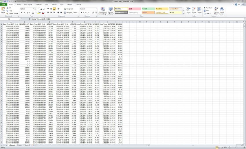
14. Open an exported .csv file, select the Date Time and when data loggers are recording highly consistent
Temp columns (fig. 2.12), then copy and paste them into temperatures. It is not possible to quantify what
columns A-B of the blank worksheet. “highly consistent” temperatures are because the
purpose of the calibration check is to look for data
15. Continue opening .csv files and copying and pasting the loggers that are dissimilar from one another and the
Date Time and Temp columns into C-D, E-F, G-H, and NIST data logger. That comparison needs to be made
so on (fig. 2.13). The header of the Temp column can be when all data loggers are recording temperatures in a
shortened to the data logger serial number (S/N). highly consistent or similar way.
16. Create a graph of data logger temperatures over time. b. Identify a period during the cold bath of greater
Make sure to include the NIST-calibrated data logger than or equal to 15 minutes (90 consecutive records)
temperatures (fig. 2.14). when data loggers are recording highly consistent
a. Identify a period during the warm bath of greater temperatures.
than or equal to 15 minutes (90 consecutive records)
Figure 2.12. Screen capture showing exported .csv file opened in Microsoft® Excel with the Date Time and Temp columns highlighted.Standard Operating Procedure (SOP) 2—Calibration Check of Data Loggers 23
Figure 2.13. Screen capture showing Microsoft® Excel with Date Time and Temp columns copied from five .csv files and pasted into
one worksheet. The Temp column headers were shortened to the data logger serial number (S/N).
Figure 2.14. Graph showing temperature over time for five Onset U22 data loggers. During
this calibration check, data loggers were placed in a warm bath before moving to a cool-
down and then a cold bath. Periods of 15 minutes (90 consecutive records) with highly
consistent temperatures are highlighted by red ovals.24 Monitoring Stream Temperatures—A Guide for Non-Specialists
17. Calculate the mean temperature for each data logger a. Accuracy for Onset U22 and TidbiT data loggers is
during that period of 90 consecutive records during the ±0.21 °C.
warm calibration.
b. Accuracy for Onset Pendant data loggers is
18. Calculate the difference between the mean temperature ±0.53 °C.
of the NIST calibrated data logger and mean temperature
of each individual data logger. c. Send inaccurate data loggers back to the
manufacturer.
a. Record that value under CalibMeanWarmDiff in the
Calibration Check Worksheet (fig. 2.1).
Procedure—Post-Field Installation Calibration
19. Calculate the mean temperature for each data logger
during that period of 90 consecutive records during the Check
cold calibration.
1. Perform a calibration check after a data logger has been
20. Calculate the difference between the mean temperature collected following field installation to check for drift in
of the NIST calibrated data logger and mean temperature temperature measurements.
of each individual data logger.
a. Drift of temperature measurements is when pre- and
a. Record that value under CalibMeanCoolDiff in the post-field calibration checks are not equal.
Calibration Check Worksheet (fig. 2.1).
2. Test the accuracy of a data logger following its field
21. Diagnose data loggers with inaccurate measurements by installation by performing the same 2-day calibration
identifying data loggers with a CalibMeanWarmDiff or check as outlined here.
a CalibMeanCoolDiff that is outside the manufacturer
specified tolerance.Standard Operating Procedure (SOP) 3—Installing Data Loggers in a Stream 25
Standard Operating Procedure (SOP) 3—Installing Data Loggers in a Stream
Overview
This SOP describes how to anchor a data logger in a stream channel for year-round data collection. This SOP also covers
which site characteristics to record to make retrieving the data logger easier.
Supplies
• Global Positioning System (GPS; pre-loaded with site coordinates in decimal degrees latitude/longitude or Universal
Transverse Mercator [UTM])
• Maps
• Stream Temperature Data Logger Installation Form (see example in appendix 1)
• Pencil
• Digital camera
• Digital thermometer
• Onset data loggers (U22, Pendant, or TidbiT)
• PVC solar shields (1 per data logger)
• 8-in. cable/zip ties (0.095 in. width; minimum two per Pendant)
• 11-in. cable/zip ties (0.18 in. width; minimum two per U22 or TidbiT)
• 36-in. cable/zip ties (0.35 in. width; three per site)
• UV resistant sand bags (two per site)
• 36-in. rebar (0.5 in. diameter; one per site)
• Rebar caps (one per piece of rebar)
• DUCKBILL Earth Anchors Model 40 (one per site)
• Driving rod for DUCKBILL Earth Anchors Model 40 (one per site)
• DUCKBILL Earth Anchors Model 68 (one per site)
• Driving rod for DUCKBILL Earth Anchors Model 68 (one per site)
• 5 lb sledge hammer
• Flagging (optional)
• Wire cutters
• Waders/wading boots or wet wading gearYou can also read