Investigating the WRF Temperature and Precipitation Performance Sensitivity to Spatial Resolution over Central Europe - MDPI
←
→
Page content transcription
If your browser does not render page correctly, please read the page content below

atmosphere

Article
Investigating the WRF Temperature and Precipitation
Performance Sensitivity to Spatial Resolution over
Central Europe
Ioannis Stergiou 1 , Efthimios Tagaris 2 and Rafaella-Eleni P. Sotiropoulou 1, *

                                          1   Department of Mechanical Engineering, University of Western Macedonia, 50132 Kozani, Greece;
                                              jstegiou@uowm.gr
                                          2   Department of Chemical Engineering, University of Western Macedonia, 50132 Kozani, Greece;
                                              etagaris@uowm.gr
                                          *   Correspondence: rsotiropoulou@uowm.gr; Tel.: +30-24610-56645

                                          Abstract: The grid size resolution effect on the annual and seasonal simulated mean, maximum and
                                          minimum daily temperatures and precipitation is assessed using the Advanced Research Weather
                                          Research and Forecasting model (ARW-WRF, hereafter WRF) that dynamically downscales the
                                          National Centers for Environmental Prediction’s final (NCEP FNL) Operational Global Analysis
                                          data. Simulations were conducted over central Europe for the year 2015 using 36, 12 and 4 km
                                          grid resolutions. Evaluation is done using daily E-OBS data. Several performance metrics and the
                                          bias adjusted equitable threat score (BAETS) for precipitation are used. Results show that model
                                          performance for mean, maximum and minimum temperature improves when increasing the spatial
                                resolution from 36 to 12 km, with no significant added value when further increasing it to 4 km.

                                          Model performance for precipitation is slightly worsened when increasing the spatial resolution from
Citation: Stergiou, I.; Tagaris, E.;
                                          36 to 12 km while further increasing it to 4 km has minor effect. However, simulated and observed
Sotiropoulou, R.-E.P. Investigating
                                          precipitation data are in quite good agreement in areas with precipitation rates below 3 mm/day
the WRF Temperature and
                                          for all three grid resolutions. The annual mean fraction of observed and/or forecast events that
Precipitation Performance Sensitivity
to Spatial Resolution over Central
                                          were correctly predicted (BAETS), when increasing the grid size resolution from 36 to 12 and 4 km,
Europe. Atmosphere 2021, 12, 278.         suggests a slight modification on average over the domain. During summer the model presents
https://doi.org/10.3390/                  significantly lower BAETS skill score compared to the rest of the seasons.
atmos12020278
                                          Keywords: WRF; Central Europe; spatial resolution; temperature; precipitation; sensitivity
Academic Editor: Anthony R. Lupo

Received: 13 January 2021
Accepted: 10 February 2021                1. Introduction
Published: 19 February 2021
                                               Earth system models (ESMs) and climate circulation models (GCMs) are still the
                                          principal tools of the scientific community for projecting future climate [1,2]. Nonetheless,
Publisher’s Note: MDPI stays neutral
                                          both are incapable of simulating local scales, as they currently resolve resolutions of
with regard to jurisdictional claims in
                                          approximately 100 km or coarser, while there are many important climate phenomena
published maps and institutional affil-
                                          that occur at spatial scales of less than 10 km (e.g., convective cloud processes, turbulence,
iations.
                                          wind patterns over complex terrain, sea breeze effects, etc.). In addition, ESMs and GCMs
                                          do not satisfactorily represent vegetation variability, complex topography and coastlines,
                                          which are significant components of the physical system that govern the climate change
                                          signal on a local or regional scale. To cope with these deficiencies, dynamical downscaling
Copyright: © 2021 by the authors.
                                          techniques have been developed and are currently adopted, for effectively adapting the
Licensee MDPI, Basel, Switzerland.
                                          large-scale projections of the inferred climate components provided by an ESM or a GCM
This article is an open access article
                                          to regional or local scales, through explicitly solving the process-based physical dynamics
distributed under the terms and
                                          of the regional climate system at high spatial resolution, when driven by the large-scale
conditions of the Creative Commons
                                          low-resolution data of the ESM/GCM [3,4].
Attribution (CC BY) license (https://
creativecommons.org/licenses/by/
                                               Regional climate models (RCMs) are among the most effective tools for dynamically
4.0/).
                                          downscaling global climate projections to local scales [5], but their ability to reproduce

Atmosphere 2021, 12, 278. https://doi.org/10.3390/atmos12020278                                        https://www.mdpi.com/journal/atmosphere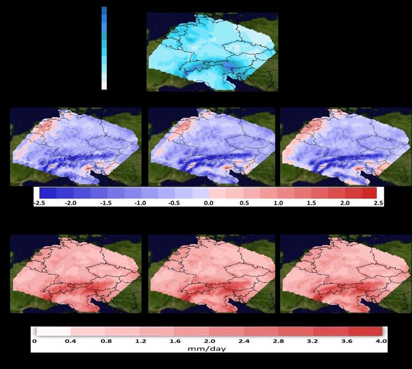
Atmosphere 2021, 12, 278                                                                                            2 of 17

                           current climate conditions needs to be evaluated, in the first place, against observations
                           before being used for such studies. This exercise allows the identification of potential
                           inherent drawbacks related to the assumptions being made by the setup of the RCM,
                           the parameterizations used and their associated uncertainties, as well as an extensive
                           evaluation of the RCM ability to reproduce significant climate features over the domain
                           of interest. Two approaches can be adopted in order to assess RCM’s ability to reproduce
                           current climate, either the use of GCM/ESM data or the use of reanalysis data as initial
                           and boundary conditions of the RCM (e.g., [6–8]). GCM/ESM data are obtained using
                           current greenhouse gases (GHG) forcings. The first approach is not flawless, given that
                           GCMs are not forced by observed data, therefore possible systematic errors developed
                           by a GCM/ESM may propagate into the RCM outputs. As a result, the added value of
                           an RCM used for downscaling purposes might be diminished. Still, such simulations are
                           very useful, as they allow climate projections and assessments for various climate change
                           scenarios on finer resolutions than those resolved by the GCMs/ESMs. On the other hand,
                           reanalysis data are the most accurate representation of the archived climate observations
                           at high temporal and spatial resolution forced by climatic observation, therefore they are
                           extensively used for evaluation purposes of the current climate.
                                 Among the climatic parameters assessed by RCMs, temperature and precipitation are
                           two parameters of crucial relevance for our societal life and the ecosystems. Being able to
                           correctly capture or project their temporal, spatial and quantitative distribution is of high
                           importance. However, their simulation is still very challenging given the wide range of
                           processes involved. Increasing the spatial resolution resolved by RCMs can, to some extent,
                           address the deficiencies in correctly capturing their temporal, spatial and quantitative
                           distribution when downscaling techniques are applied. Multi-nesting approaches in
                           downscaling procedures can add more detail in the assessments, ensuring at the same
                           time that the outputs at the finer scales resolved by the nests of the RCM are dynamically
                           consistent with the large-scale flows. However, the use of several consecutive nests is
                           both a computationally demanding process and does not assure a perfect replicability,
                           degradation or improvement by the RCM outputs. As a result, a number of studies have
                           been conducted assessing the spatial resolution effect, when multi-nesting approaches are
                           used, on models’ performances.
                                 Long term studies have been conducted over Europe, reaching up to 12 km grid-point
                           distance. Vautard et al. [9] examined heatwave prediction within the EURO-CORDEX
                           project at 50 and 12 km resolutions using a multi-model ensemble. They found that
                           there is no significant improvement in maximum temperature prediction, especially in
                           mountainous regions. Kotlarski et al. [10], within the same framework, examined air
                           temperature and precipitation at grid resolutions of 50 and 12 km and could not find clear
                           benefit by the increase in the grid spacing. This was also the conclusion of Jaeger et al. [11]
                           for temperature and precipitation within the ENSEMBLES project at 0.44◦ and 0.22◦ spatial
                           resolutions as well as van Roosmalen et al. [12] for Denmark. However, Heikkilä et al. [13]
                           found noteworthy added value comparing 30 and 10 km simulations over Norway.
                                 A number of studies [14–16] focus only on precipitation sensitivity with respect to
                           various spatial resolutions and regions. Their results address the estimated biases which
                           do not seem to be clearly improved. Giorgi and Marinucci [14] found that precipitation
                           amount, intensity, and distribution depend on the grid size. Leung and Qian [15] found
                           that the increase of the resolution (from 40 to 13 km) did not cause a uniform improvement
                           of precipitation assessments over complex terrains. Li et al. [16] found that increasing the
                           horizontal resolution from 30 to 10 km improved the forecasting ability for precipitation.
                           Rauscher et al. [17] in the framework of the ENSEMBLES project found that both patterns
                           and temporal evolution of precipitation during summer are improved when decreasing
                           grid spacing from 50 to 25 km. Chan et al. [18] also found added value in capturing
                           precipitation events in topographically complex regions as a result of decreasing grid
                           spacing. Precipitation spatial pattern representation is improved but only a small or
                           not significant improvement can be detected for mean biases along coastlines [7]. Prein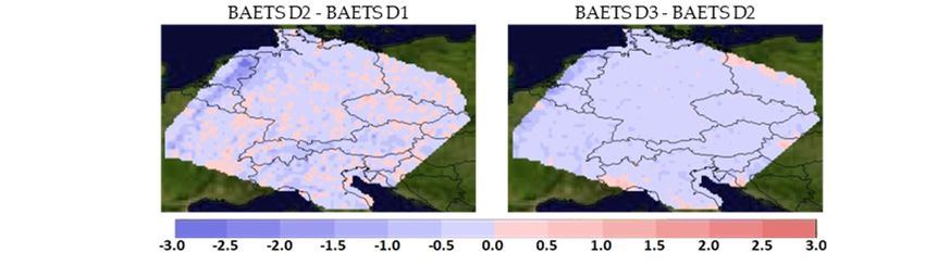
Atmosphere 2021, 12, 278                                                                                            3 of 17

                           et al. [19] examined the representation of mean and extreme precipitation within the EURO-
                           CORDEX project at 0.44◦ and 0.11◦ resolutions and found that increased resolution adds
                           value, while in regions with complex terrain (e.g., Alps, the Carpathian) added value in
                           precipitation biases tends to cancel out by averaging. Similar were the findings of Torma
                           et al. [20] within the EURO-CORDEX framework that found improvement in the spatial
                           representation and the extremes of precipitation at finer grid resolutions.
                                 Despite the large number of studies examining the effect of the spatial resolution on
                           models’ performances, the question of up to what spatial scales downscaling global data
                           to local scales can actually improve local representation of temperature and precipitation
                           and whether very fine resolutions (below 10 km) are necessary for their improved repre-
                           sentation still remains inadequately addressed. Addressing this challenge, in this study
                           we assess the Advanced Research Weather Research and Forecasting model (ARW-WRF,
                           hereafter WRF) [21,22] temperature and precipitation performance sensitivity to the grid
                           size resolution. Performance sensitivity is examined for WRF downscaled simulated mean,
                           maximum and minimum daily temperatures as well as precipitation and we compare the
                           model’s predictions against daily data from the E-OBS data base [23], in order to draw
                           conclusions on the added value of their representation in higher grid size resolution scales.
                           The grid size resolutions selected here, i.e., 36, 12, and 4 km, extend beyond the typical size
                           of 0.11◦ (~12 km) used in previous studies (e.g., [24–26]). The selected domain is extended
                           over central Europe, due to the significant number of observational data, for assessing both
                           annual and seasonal impact.

                           2. Materials and Methods
                           2.1. Modeling Setup
                                The Weather Research and Forecasting (WRF) model [21,22] version 3.9.1 is used to
                           simulate meteorological variables. WRF is one of the most widely used Regional Climate
                           Models (RCMs) for downscaling global data to regional scales. It is a mesoscale numerical
                           weather prediction system used for reproducing local weather and climate at high spatial
                           resolutions. It has extensively been used for climate and meteorological applications over
                           Europe (e.g., [25–27]).
                                In this study, the parent-coarse model domain is centered at (49◦ N, 10.5◦ E) and consists
                           of 50 grid cells east and north with a grid cell size of 36 km. The two nested domains have
                           100 and 250 grid cells in the west–east and south-north direction with grid cell sizes of
                           12 and 4 km, respectively. The finer nested domain covers the central European region
                           (Figure 1). The nests are one-way interactive to avoid feedback of the inner to the outer
                           domains so that the results represent the resolution effect only. In the vertical direction,
                           the model used 40 layers. The NCEP FNL (Final) Operational Model Global Tropospheric
                           Analyses data at 1-degree resolution are used as the single initial and lateral boundary
                           conditions for the parent domain, while the latter is updated every 6 hours throughout
                           the model simulations. The modeling setup is similar to the one used in the WRF EURO-
                           CORDEX framework [10,25] for all grid resolutions, employing the WSM-5 microphysics
                           scheme, the RRTMG radiation scheme, the YSU PBL scheme, and the NOAH land surface
                           scheme. Simulations cover the period July 2014 to December 2015, with a 6 month period
                           being used as a spin-up time, allowing a more realistic development of snow cover [28].

                           2.2. Observational Data
                               Comparison between predicted and observed values for mean, maximum, minimum
                           temperatures and precipitation is performed for the year 2015 using daily data from the
                           E-OBS dataset [[23,29]. The E-OBS data are based on the European Climate Assessment
                           and Dataset (ECA&D) project station observation data (https://www.ecad.eu/download/
                           ensembles/download.php#datafiles (accessed on 5 February 2021)) that covers the entire
                           European domain. The E-OBS dataset has extensively been used in the past for comparison
                           studies over Europe (e.g., [10,26,30–35]). To evaluate model performance, results were
                           compared with the ensemble mean of the regular 0.25◦ grid version of the E-OBS v20.0e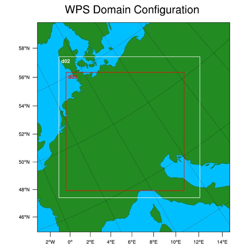
Atmosphere 2021, 12, 278                                                                                                         4 of 17

                                       observational dataset. Therefore, the E-OBS grid of 0.25-degree is used as a reference upon
                                       which all WRF domain grids are interpolated. After interpolating model-derived temper-
                                       ature, and precipitation to the E-OBS grid within the investigation area, i.e., D3 domain,
                                       mean, maximum, minimum temperatures, and precipitation were calculated. One could
                                       argue that the specific database is too coarse to compare against the finer domain’s outputs,
                                       however, as pointed out by Prein et al, [19] and Fantini et al, [36], it is anticipated that if
                                       processes are captured better at higher resolution, improvements are still visible when
Atmosphere 2021, 12, x FOR PEER REVIEW regridded to coarser resolution. As a result, in order to assure a fair intercomparison
                                                                                                                           4 of among
                                                                                                                                18

                                       the three grid resolutions, we chose to regrid variables to the grid of E-OBS.

                                     Figure
                                Figure      1. Weather
                                       1. Weather      Research
                                                  Research      and Forecasting
                                                           and Forecasting    (WRF)(WRF)   multi-nesting
                                                                                     multi-nesting domaindomain  configuration
                                                                                                           configuration       approach
                                                                                                                         approach
                                     with increasing
                                with increasing      domain
                                                domain      resolution
                                                       resolution of 36,of1236,
                                                                             and124and
                                                                                    km.4 km.

                                            DespiteData
                                2.2. Observational     the extensive use of the E-OBS database, there are some known shortfalls
                                      related to the spatial coverage of its network stations and the quality of the data where
                                      Comparison between predicted and observed values for mean, maximum, minimum
                                      sparse density of stations exist, affecting the magnitude of daily extremes in temperature
                                temperatures and precipitation is performed for the year 2015 using daily data from the
                                      (e.g., [32,37–41]) and possibly the total precipitation that is underpredicted [41], especially
                                E-OBS dataset [[23,29]. The E-OBS data are based on the European Climate Assessment
                                      in mountainous and snow-covered regions [42]. However, given that E-OBS has a dense
                                and Dataset (ECA&D) project station observation data (https://www.ecad.eu/down-
                                      station network with good temporal coverage over central Europe, it has been selected for
                                load/ensembles/download.php#datafiles) that covers the entire European domain. The E-
                                      our study, as its known inefficiencies will not affect the comparison with our simulated data.
                                OBS dataset has extensively been used in the past for comparison studies over Europe
                                (e.g.,2.3.
                                       [10,26,30–35]).
                                           PerformanceTo    evaluate model performance, results were compared with the en-
                                                          Metrics
                                semble mean       of the regular  0.25° grid version of the E-OBS v20.0e observational dataset.
                                            Mean bias (MB), separated into positive and negative biases for avoiding any mislead-
                                Therefore,     the E-OBS   grid of 0.25-degreeof
                                      ing results due to counterbalancing        is positive
                                                                                    used as and
                                                                                             a reference
                                                                                                  negative upon which
                                                                                                            values,  meanall absolute
                                                                                                                             WRF do-error
                                main(MAE),
                                       grids are   interpolated.
                                                 root mean square After  interpolating
                                                                     error (RMSE) andmodel-derived        temperature,
                                                                                         the index of agreement    (IoA)and   precipi-
                                                                                                                          (Table  1) are the
                                tationstatistical
                                        to the E-OBS     grid within   the investigation  area, i.e., D3 domain,  mean,    maximum,
                                                   indices used in order to assess the impact of grid size resolution on the model’s
                                minimum       temperatures,
                                      simulated               and
                                                    outputs for    precipitation
                                                                temperature    andwere   calculated.These
                                                                                     precipitation.   One could  argue
                                                                                                            metrics  are that the used
                                                                                                                         widely   spe- and
                                cific database is too coarse to compare against the finer domain’s outputs, however, as
                                pointed out by Prein et al, [19] and Fantini et al, [36], it is anticipated that if processes are
                                captured better at higher resolution, improvements are still visible when regridded to
                                coarser resolution. As a result, in order to assure a fair intercomparison among the three
                                grid resolutions, we chose to regrid variables to the grid of E-OBS.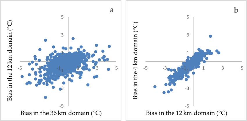
Atmosphere 2021, 12, 278                                                                                                                                       5 of 17

                           simply reproducible allowing in a rigorous way the assessment of the model performance.
                           The statistical analysis is based on the daily values for each individual model grid cell
                           assessing both annual and seasonal impacts. In Table 1, Xpredicted and Xobserved stand for the
                           daily gridded predicted and observed values, with n being the total number of grid points,
                           while overbars denote mean values.

                           Table 1. Statistical Measures.
                                                    n
                                                 ∑i=1 ( X predicted − Xobserved )
                            Mean Bias (MB) =                    n
                                                                       n
                                                                      ∑ |X          − Xobserved |
                            Mean Absolute    Error (MAE) = i=1 rpredicted         n
                                                                                 n                             2
                                                                               ∑i=1 ( X predicted − Xobserved )
                            Root Mean Square Error (RMSE) =                                    n
                                                                                       n                             2
                                                                                    ∑i=1 ( X predicted − Xobserved )
                            Index of Agreement (IoA) = 1 −               n                                                              2
                                                                       ∑i=1 (| X predicted − X observed |+| Xobserved − X observed |)

                                In addition, the bias adjusted equitable threat score (BAETS) [43] for precipitation
                           is used in order to assess how well the forecast “yes” correspond to the observed “yes”
                           events. Table 2 presents the 2 × 2 contingency table in the form required for this analysis,
                           used in verifying dichotomous forecasts.

                           Table 2. Contingency table illustrating the counts used for bias adjusted equitable threat score
                           (BAETS) calculation.

                                                                                               Observed
                                                                                     Yes                              No                           Total
                                                                                     Hits                       False alarms                    Forecast Yes
                                                        Yes
                                Forecast                                             (H)                            (Z)                         (F = H + Z)
                                                                                 Misses                     Correct negatives                   Forecast No
                                                        No
                                                                                  (Y)                             (W)                            (Y + W)
                                                                             Observed Yes                      Observed No                         Total
                                           Total
                                                                             (O = H + Y)                        (Z + W)                     (N = H + Z + Y + W)

                                The BAETS is given by the formula:

                                                                                                HA − F O
                                                                                                       N
                                                                    BAETS =                                                                                       (1)
                                                                                       F + O − HA − F O
                                                                                                      N

                           where HA is the bias adjusted number of hits (H),

                                                          F−H

                                                                              O        O
                                             HA = O −           lambertw       ln                                                                               (2)
                                                            O
                                                        ln O−                F−H      O−H
                                                              H

                           where lambertw stands for the Lambert W-function or omega function, F denotes the forecast
                           event (correctly forecast area or “hits” plus the “false alarms”), O denotes the observed
                           area and N denotes the total number of verification points or events. BAETS has a value
                           between −1 /3 and 1, with 0 indicating no skill and 1 is the perfect score.

                           3. Results and Discussion
                           3.1. Mean Temperature
                                The model reproduces the observed annual domain mean temperature over all three
                           grid size resolutions used in this study. As can be seen in Table 3, there is an average
                           underestimation of the observed mean temperature of 0.13 ◦ C for the 36 km grid size
                           domain (D1), of 0.12 ◦ C on average for the 12 km grid size domain (D2), and of 0.10 ◦ C on
                           average for the 4 km grid size domain (D3). An overestimation is found mainly over the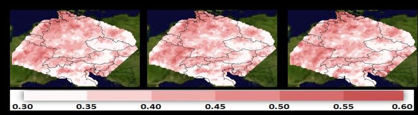
3.1. Mean Temperature
The model reproduces the observed annual domain mean temperature over all three
grid size resolutions used in this study. As can be seen in Table 3, there is an average
Atmosphere 2021, 12, 278 underestimation of the observed mean temperature of 0.13 °C for the 36 km grid 6size of 17
domain (D1), of 0.12 °C on average for the 12 km grid size domain (D2), and of 0.10 °C on
average for the 4 km grid size domain (D3). An overestimation is found mainly over the
north and northeast region of the domain and an underestimation over the southern part
ofnorth and northeast
the domain. region of
This finding, i.e.,the
thedomain andatan
cold bias theunderestimation
north and the warm over the
biassouthern part
at the south
of the domain. This finding, i.e., the cold bias at the north and the warm
part of Europe has also been stated in other RCM studies [10,26]. The highest positive and bias at the south
part of Europe
negative has also
differences are been
found stated in other
in regions RCM studiesby
characterized [10,26].
complexTheorographic
highest positive and
features,
negative differences are found in regions characterized by complex orographic
e.g., the Alps and northern Italy (Figure 2). This trend, as well as the spatial pattern, do features,
e.g.,change,
not the Alpsinand northern
general, Italythe
with (Figure 2). This
increase trend,
in the as well
spatial as the spatial
resolution. pattern,model
However, do not
change, in general,
performance with
is better whenthedecreasing
increase in the the spatial resolution.
grid spacing from However,
36 (D1) tomodel
12 km performance
(D2) but no
is better when decreasing the grid spacing from 36 (D1) to 12 km
significant change is found when the spatial resolution is further increased (i.e., (D2) but no significant
4 km
change
(D3)). is found when the spatial resolution is further increased (i.e., 4 km (D3)).
Tobs
Tobs-TD1 Tobs-TD2 Tobs-TD3
MAED1 MAED2 MAED3
Figure
Figure 2. Spatial distribution plots 2.
forSpatial
annualdistribution plots forobserved
mean temperature: annual mean temperature:
data (upper panel), observed
differencesdata (upper
between panel),
observed
differences between observed and simulated data for the three nested domains (middle
and simulated data for the three nested domains (middle row), and the related mean absolute error (MAE) (lower row). row), and
the related mean absolute error (MAE) (lower row).
This is also supported by the domain wide average values of the statistical measures
This is also
for D1-D3 supported
(Table 3). Thesebymeasures
the domain wide
show average values
statistically of the improvement
significant statistical measures
in the
for D1-D3
biases, the(Table
RMSE3). andThese measures
the MAE whenshow statistically
increasing significant
the spatial improvement
resolution from 36 to in 12 the
km,
biases,
while athe RMSE
minor and the MAE
improvement when
is seen increasing
with the spatial
further increase resolution
of the from
resolution to 436km.
to 12 km,a
From
while a minor
statistical improvement
point of view, thisisimplies
seen with
thatfurther increase
simulations of athe
with resolution
grid size of 12tokm4 km. From
might be
aadequate
statisticaltopoint of view, this implies that simulations with a grid size of 12 km
describe annual temperature trends, derived from daily data, over large regions, might be
avoiding computationally demanding simulation with fine grid spacing. Comparing the
grid data between domains D1 against D2 and D2 against D3 (Table 3, columns ∆ij (D2-D1)
and ∆ij (D3-D2)) it is clear that there is a statistically significant change on the average
values of biases and RMSE between D1 and D2, and a minor change between D2 and D3
with the reduction of the grid resolution. The better closure between D2 and D3 grid data
implies that there is no clear statistical evidence of improvement when downscaling data
to the finer grid resolution used here (i.e., 4 km).
adequate to describe annual temperature trends, derived from daily data, over large re-
gions, avoiding computationally demanding simulation with fine grid spacing. Compar-
Atmosphere 2021, 12, 278 ing the grid data between domains D1 against D2 and D2 against D3 (Table 3, columns 7 of 17
Δij(D2-D1) and Δij(D3-D2)) it is clear that there is a statistically significant change on the
average values of biases and RMSE between D1 and D2, and a minor change between D2
and D3 with the reduction of the grid resolution. The better closure between D2 and D3
Table 3. Annual mean temperature statistical analysis (◦ C).
grid data implies that there is no clear statistical evidence of improvement when
downscaling data to the finer
D1 grid resolution
D2 used here
D3 (i.e., 4 km).
∆ij (D2-D1) ∆ij (D3-D2)
(36 km) (12 km) (4 km)
Table 3. Annual
Mean Observed mean temperature statistical
10.22analysis (°C). - -
Mean Predicted D1
10.09 10.10D2 D3
10.12 - -
Δij (D2-D1) Δij (D3-D2)
(36 km) (12 km) (4 km)
Positive MB
Mean Observed
0.48 0.34
10.22
0.32 0.40
-
0.13
-
Negative MB
Mean Predicted −0.69
10.09 −0.53
10.10 −0.52
10.12 −0.39
- −0.09
-
Positive ΜΒ 0.48 0.34 0.32 0.40 0.13
RMSE 0.87 0.61 0.59 0.72 0.19
Negative ΜΒ −0.69 −0.53 −0.52 −0.39 −0.09
IoA
RMSE 0.970.87 0.98
0.61 0.99
0.59 0.98
0.72 1
0.19
MAEIoA 0.590.97 0.98
0.44 0.99
0.43 0.98
0.39 1
0.10
MAE 0.59 0.44 0.43 0.39 0.10
Investigating the
Investigating the climatological
climatological variability
variability of
of annual
annual average
average temperatures
temperatures inin combi-
combi-
nation with the grid size effect, we compare the grid biases, i.e., simulated minus
nation with the grid size effect, we compare the grid biases, i.e., simulated minus observed observed
daily values
daily values for
foreach
eachgrid,
grid,for
for domains
domains D1D1 against
against D2 D2 (Figure
(Figure 3a) and
3a) and D2 against
D2 against D3
D3 (Fig-
(Figure 3b). The D2 simulation tends to reduce biases compared to D1 with
ure 3b). The D2 simulation tends to reduce biases compared to D1 with slightly higher slightly higher
temperatures (below
temperatures (belowthe thediagonal).
diagonal).TheThebiases between
biases betweenthethe
D2 D2andandD3 simulations are very
D3 simulations are
similar (mostly fall on the diagonal) and smaller in range than the D1 simulation (Figure 3).
very similar (mostly fall on the diagonal) and smaller in range than the D1 simulation
As a result, the improvement is higher for D2 compared to D1, with no significant added
(Figure 3). As a result, the improvement is higher for D2 compared to D1, with no signif-
value being seen for D3 compared to D2.
icant added value being seen for D3 compared to D2.
Figure 3. Scatter plots presenting (a) D1 (x-axis) against D2 (y-axis) and (b) D2 (x-axis) against D3
Figure 3. Scatter plots presenting (a) D1 (x-axis) against D2 (y-axis) and (b) D2 (x-axis) against D3 (y-axis) simulated annual
(y-axis) simulated annual temperature biases for all grids considered.
temperature biases for all grids considered.
In addition, the
In addition, the spatial
spatial error
error variability, defined as
variability, defined as the
the difference
difference between
between the
the first
first
(25th) and third (75th) quartile, is derived for the three domain resolutions. Results
(25th) and third (75th) quartile, is derived for the three domain resolutions. Results show show
improvement
improvement in in the
the spatial
spatial error
error variability
variability (0.85
(0.85 ◦°C for D1,
C for D1, 0.70
0.70 ◦°C for D2
C for D2 and
and 0.68
0.68 ◦°C for
C for
D3)
D3) with
with the
the reduction
reduction ofof the
the grid
grid resolution.
resolution. Although
Although aa clear improvement is
clear improvement is seen
seen when
when
comparing
comparing D1D1 against D2, there
against D2, is no
there is no clear
clear evidence
evidence of of improvement
improvement when when comparing
comparing D2 D2
against D3. These findings also support the conclusion derived from the statistical analysis
that simulations with a grid size resolution of 12 km are sufficient for describing annual
temperature trends over large domains.
The seasonal mean temperature plots present a similar spatial pattern between the
three domains for each season (Figures S1–S4 of Supplementary Material). During autumn,
Atmosphere 2021, 12, 278                                                                                                         8 of 17

                                  the model, for all grid resolutions, overestimates mean temperature over a major part of
                                  the domain and underestimates it mainly over the northwest and central parts of Italy
                                  (Figure S1). Increasing the spatial resolution from 36 (D1) to 4 km (D3) improves the
                                  statistical metrics (Table S1), suggesting that the finer domain better represents autumn
                                  mean temperature. This is related to both the positive and negative MBs which are
                                  improved when moving from the coarser to the finer resolution. During winter the model,
                                  in all three grid resolutions, underestimates mean temperature mainly over northwest Italy
                                  and the region over the Alps (Figure S2). Increasing the spatial resolution from 36 (D1)
                                  to 12 km (D2) leads to improved statistical measures (Table S2) but no significant change
                                  is found when the spatial resolution is further increased (i.e., 4 km (D3)). During spring
                                  and summer, the model, in all grid resolutions, underestimates mean temperature in most
                                  parts of the domain with an exception of the north–northeast region (Figures S3 and S4).
                                  Increasing the spatial resolution from 36 (D1) to 12 km (D2) leads to improved statistical
                                  measures (Tables S3 and S4) but no significant change is found when the spatial resolution
                                  is further increased (i.e., 4 km (D3)).

                                  3.2. Maximum Temperature
                                           The model underestimates annual maximum temperature in a major part of the
                                    domain. The highest differences are found in the Alps region (Figure 4). This trend,
                                    as well as the spatial pattern, do not change with the increase of the spatial resolution.
                                    However, model performance is better when increasing the spatial resolution from 36 (D1)
                                    to 12 km (D2), while a minor change is found when the spatial resolution is further increased
                                    (i.e., 4 km (D3)). This is also supported by the domain wide average values of the 9statistical
  Atmosphere 2021, 12, x FOR PEER REVIEW                                                                                  of 18
                                    metrics (Table 4).

                                                                 TXobs

                           TXobs-TXD1                        TXobs-TXD2                            TXobs-TXD3

                            MAED1                              MAED2                                MAED3

      Figure 4. Spatial distribution plots for annual max temperature: observed data (upper panel), differences between observed
      and simulated data for the three   nested
                                    Figure       domains
                                            4. Spatial       (middleplots
                                                       distribution   row),
                                                                          forand the related
                                                                              annual         MAE (lower
                                                                                     max temperature:   row). data (upper panel),
                                                                                                      observed
                                    differences between observed and simulated data for the three nested domains (middle row), and
                                    the related MAE (lower row).

                                  Table 4. Annual maximum temperature statistical analysis (°C).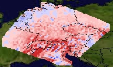
Atmosphere 2021, 12, 278                                                                                              9 of 17

                           Table 4. Annual maximum temperature statistical analysis (◦ C).

                                                      D1            D2             D3
                                                                                             ∆ij (D2-D1)   ∆ij (D3-D2)
                                                    (36 km)       (12 km)        (4 km)
                              Mean Observed                         14.91                         -             -
                              Mean Predicted         14.33          14.41         14.44           -             -
                               Positive BIAS          0.40          0.24           0.23         0.49           0.14
                              Negative BIAS          −0.87         −0.68          −0.64        −0.50          −0.11
                                  RMSE                1.14          0.81           0.76         0.82           0.22
                                    IoA               0.95          0.98           0.99         0.98           1.00
                                   MAE                0.76          0.59           0.56         0.49           0.13

                                The seasonal maximum temperature plots present a similar spatial pattern between the
                           three domains for each season (Figures S5–S8 of Supplementary Material). During autumn,
                           the model overestimates maximum temperature over the domain with the exception
                           of the Alps region (Figure S5). Increasing the spatial resolution from 36 (D1) to 4 km
                           (D3) improves the statistical measures (Table S5) suggesting that the finer domain better
                           represents autumn maximum temperature. However, the improvement between 36 (D1)
                           and 12 km (D2) is more important compared to the improvement between 12 (D2) and 4 km
                           (D3). During winter, the model underestimates maximum temperature in major part of the
                           domain (Figure S6). Underestimation is mainly noted over Italy, the Eastern Alps and most
                           part of Switzerland. Increasing the spatial resolution from 36 (D1) to 12 km (D2) improves
                           the statistical measures (Table S6) but no significant change is found when the spatial
                           resolution is further increased (i.e., 4 km (D3)). During spring and summer, the model
                           underestimates maximum temperature in most parts of the domain (Figures S7 and S8).
                           Increasing the spatial resolution from 36 (D1) to 12 km (D2) improves statistical measures
                           (Tables S3 and S4) but no significant change is found when the spatial resolution is further
                           increased (i.e., 4 km (D3)).

                           3.3. Minimum Temperature
                                The model underestimates annual minimum temperature in major part of the domain
                           for all three grid resolutions used. The highest differences are found over northern Italy
                           and the Alps region (Figure 5). This trend, as well as the spatial pattern, do not change with
                           the increase of the spatial resolution. Model performance does not change in the higher
                           spatial resolution grids (i.e., 12 (D2) and 4 km (D3)) compared to the 36 km (D1) domain,
                           except for the positive bias that is improved on the finer nested domain (Table 5).

                           Table 5. Annual minimum temperature statistical analysis (◦ C).

                                                      D1            D2             D3
                                                                                             ∆ij (D2-D1)   ∆ij (D3-D2)
                                                    (36 km)       (12 km)        (4 km)
                              Mean Observed                         5.73                          -             -
                              Mean Predicted          5.23          5.11           5.00           -             -
                               Positive BIAS          0.55          0.44           0.39         0.40           0.12
                              Negative BIAS          −1.00         −1.00          −1.07        −0.35          −0.14
                                  RMSE                1.27          1.27           1.31         0.63           0.21
                                    IoA               0.92          0.92           0.92         0.98           1.00
                                   MAE                0.85          0.85           0.91         0.35           0.14
3.3. Minimum Temperature
                                       The model underestimates annual minimum temperature in major part of the
                                  domain for all three grid resolutions used. The highest differences are found over northern
                                  Italy and the Alps region (Figure 5). This trend, as well as the spatial pattern, do not
Atmosphere 2021, 12, 278          change with the increase of the spatial resolution. Model performance does not change       in17
                                                                                                                          10 of
                                  the higher spatial resolution grids (i.e., 12 (D2) and 4 km (D3)) compared to the 36 km (D1)
                                  domain, except for the positive bias that is improved on the finer nested domain (Table 5).

                                                                   TNobs

                           TNobs-TND1                          TNobs-TND2                             TNobs-TND3

                            MAED1                                MAED2                                  MAED3

      Figure 5. Spatial distribution plots for annual minimum temperature: observed data (upper panel), differences between
      observed and simulated dataFigure  5. Spatial
                                     for the        distribution
                                             three nested        plots
                                                           domains     for annual
                                                                    (middle  row),minimum    temperature:
                                                                                   and the related        observed
                                                                                                   MAE (lower  row).data (upper
                                 panel), differences between observed and simulated data for the three nested domains (middle
                                         Thethe
                                 row), and    seasonal
                                                related minimum
                                                         MAE (lower temperature
                                                                       row).      plots present a similar spatial pattern between the
                                    three domains for each season (Figures S9–S12 of Supplementary Material). For all seasons,
                                  Table
                                   mean 5. predicted
                                           Annual minimum
                                                     values temperature statistical
                                                             are lower than         analysis (°C).
                                                                              the observed     ones, with domain D1 presenting a
                                    better closure with observations
                                                                  D1     compared
                                                                               D2 to D2 andD3    D3, mainly as a result of the gradual
                                    increase in the negative bias     when moving
                                                                (36 km)      (12 km) from D1    to D2 andΔD3.
                                                                                            (4 km)
                                                                                                            ij (D2-D1)      Δij (D3-D2)
                                                                                                                   This finding   might be
                                    related
                                        Meanto  the stronger negative bias in precipitation
                                              Observed                         5.73          (Tables S13–S16)     - when moving   - to finer
                                    gridMean
                                          resolutions
                                              Predicted that leads  to gradually
                                                                  5.23            larger evaporative
                                                                               5.11           5.00      cooling.  - During autumn -      the
                                    modelPositive BIAS
                                            overestimates         0.55
                                                            min temperature    0.44 the eastern
                                                                              over            0.39border of the 0.40
                                                                                                                   domain and 0.12
                                                                                                                                 north-east
                                    Italy (Figure S9). Increasing the spatial resolution does not improve the statistical measures
                                    except for the positive bias (Table S9). During winter the model underestimates min
                                    temperature mainly over north-west Italy and the Alps region while there is a mixed trend
                                    for the rest of the domain (Figure S10). Increasing the spatial resolution from 36 (D1) to 4 km
                                    (D3) causes a slight improvement on the positive bias but the rest of the statistical measures
                                    do not improve (Table S10). During spring and summer, the model underestimates min
                                    temperature in most part of the domain (Figures S11 and S12). Increasing the spatial
                                    resolution from 36 (D1) to 4 km (D3) does not improve the statistical measures except for
                                    the positive bias (Table S1).

                                    3.4. Precipitation
                                         The model overestimates annual precipitation in major part of the domain except
                                    the regions at the west and south east borders (Figure 6). Simulated and observed data
                                    are in quite good agreement in areas with precipitation rates below 3mm/day with the
Atmosphere 2021, 12, 278 11 of 17
model being able to represent the precipitation range within a ±25% accuracy. However,
for high-precipitation areas such as the alpine and mountainous regions, differences are
quite high (up to 2.5 mm/day overestimation by the model) that are probably related
to known E-OBS deficiencies in properly capturing the correct range of precipitation in
Atmosphere 2021, 12, x FOR PEER REVIEW
regions with sparse and uneven station coverage. This trend as well as the spatial 12 of 18
pattern
do not change with the increase of the spatial resolution.
Figure 6. Spatial distribution plots for annual mean precipitation: observed data (upper panel), differences between
observed and simulated data for the
Figure three nested
6. Spatial domains
distribution (middle
plots row),mean
for annual and the related MAE
precipitation: (lower row).
observed data (upper panel),
differences between observed and simulated data for the three nested domains (middle row), and
The MAE
the related statistical
(loweranalysis
row). suggests that model performance is slightly better when in-
creasing the spatial resolution from 36 (D1) to 12 km (D2) while further increasing spatial
resolution to 4 kmanalysis
The statistical (D1) hassuggests
a negligible
that effect
model(Table 6). Minorisimprovements
performance slightly betterinwhen mod-
els’ performances on a daily, seasonal or annual basis when increasing
increasing the spatial resolution from 36 (D1) to 12 km (D2) while further increasing the grid spac-
spatial resolution to 4 km (D1) has a negligible effect (Table 6). Minor improvementswell
ing to convection permitting simulations have also been found by other studies as in
(e.g., [18,24,44,45])
models’ performancessuggesting
on a daily,thatseasonal
sub-dailyortimeframes
annual basis need to beincreasing
when considered theingrid
such
cases for
spacing toimprovements to be seen.
convection permitting simulations have also been found by other studies as
Investigating
well (e.g., the grid
[18,24,44,45]) size effect,
suggesting that we compare
sub-daily the biases,need
timeframes i.e., to
simulated minus in
be considered ob-
served daily values, for domains
such cases for improvements to be seen. D1 against D2 (Figure 7a) and D2 against D3 (Figure 7b).
The biases between the D2 and D3 simulations are very similar (mostly fall on the diagonal)
Table 6.slightly
with Annuallower precipitationstatistical
mean precipitation rates foranalysis
D3 domain (below the diagonal) and smaller in
(mm/day).
range than the D1 simulation (Figure 7a). As a result, the projection improvement is higher
D1 D2 D3
for D2 compared to D1, with no significant added value being seen for D3 compared
Δij (D2-D1) to D2.
Δij (D3-D2)
(36 km) (12 km) (4 km)
In addition, the spatial error variability
Mean Observed
derived for the three domain
1.97 -
resolutions -
shows
Mean Predicted 2.49 2.48 2.42 - -
Positive MB 0.67 0.66 0.65 0.00 0.66
Negative MB −0.38 −0.35 −0.33 4.97 −2.51
RMSE 0.81 0.80 0.79 2.44 −0.48
IoA 0.77 0.78 0.79 −0.74 0.12Atmosphere 2021, 12, 278 12 of 17
only a minor improvement in the spatial error variability (0.58 mm/d for D1, 0.56 mm/d
for D2 and 0.55 mm/d for D3) with the reduction of the grid resolution.
Table 6. Annual mean precipitation statistical analysis (mm/day).
Atmosphere 2021, 12, x FOR PEER REVIEW 13 of 18
D1 D2 D3
∆ij (D2-D1) ∆ij (D3-D2)
(36 km) (12 km) (4 km)
Investigating
Mean Observed the grid size effect,1.97we compare the biases, i.e.,- simulated minus - ob-
served daily values,
Mean Predicted for domains
2.49 D1 against
2.48 D2 (Figure
2.42 7a) and D2 against
- D3 (Figure
- 7b).
The biases between the D2 and D3 simulations are very similar (mostly fall on the diago-
Positive MB 0.67 0.66 0.65 0.00 0.66
nal) with slightly lower precipitation rates for D3 domain (below the diagonal) and
Negative
smaller MB than the
in range −0.38 −0.35
D1 simulation −0.33
(Figure 7a). the projection−improve-
As a result, 4.97 2.51
ment isRMSE
higher for D2 compared
0.81 to D1,0.80
with no significant
0.79 added2.44 −0.48
value being seen for D3
compared IoAto D2. In addition,
0.77 the spatial
0.78 error variability
0.79 derived
−0.74for the three domain
0.12
resolutions shows only a minor improvement in the spatial error variability (0.58 mm/d
MAE 0.62 0.62 0.60 0.96 −1.39
for D1, 0.56 mm/d for D2 and 0.55 mm/d for D3) with the reduction of the grid resolution.
Figure(a)7.D1
Figure 7. Scatter plots presenting Scatter plots
(x-axis) presenting
against (a) D1and
D2 (y-axis) (x-axis)
(b) D2against
(x-axis)D2 (y-axis)
against D3and (b) D2
(y-axis) (x-axis) against
simulated annual D3
(y-axis) simulated annual precipitation biases for all grid cells considered.
precipitation biases for all grid cells considered.
The
The seasonal
seasonalprecipitation
precipitationplots
plotspresent
presenta similar spatial
a similar spatialtrend between
trend betweenthe the
three do-
three
mains for each season (Figures S13–S16 of Supplementary Material).
domains for each season (Figures S13–S16 of Supplementary Material). During autumn, During autumn, the
model underestimates precipitation mainly at the north-west and
the model underestimates precipitation mainly at the north-west and south-east part ofsouth-east part of the
domain
the domain (Figure S13)S13)
(Figure in all
inresolutions
all resolutionsconsidered, while
considered, the statistical
while analysis
the statistical suggests
analysis sug-
negligible effect effect
gests negligible of theofgrid
the size
grid on
sizethe
onresults (Table
the results S13).S13).
(Table During winter
During the model
winter un-
the model
derestimates
underestimates precipitation
precipitationmainly at the
mainly north-west
at the north-westpartpart
of the
of domain
the domain(Figure S14).S14).
(Figure The
statistical
The analysis
statistical suggests
analysis that model
suggests performance
that model is negligibly
performance affectedaffected
is negligibly when increasing
when in-
the spatial resolution from 36 (D1) to 12 km (D2), while further
creasing the spatial resolution from 36 (D1) to 12 km (D2), while further increasingincreasing to 4 km
to 4(D3)
km
spatial
(D3) resolution
spatial does does
resolution not improve statistics
not improve (Table(Table
statistics S14). S14).
During spring,
During the model
spring, over-
the model
estimates
overestimatesprecipitation at major
precipitation part
at major partof of
thethe
domain
domain(Figure
(FigureS15).
S15).TheThe statistical analysis
statistical analysis
suggests that increasing the spatial resolution from 36 (D1) to 12 km (D2) as well as from
12 (D2) to 4 km (D3) does not modify modify significantly model performance. During summer,
the model overestimates precipitation
precipitation at at major
major parts
parts of the domain with the largest values
over the high elevated regions of northern Italy (Figure S16). This positive bias is caused
by the
the cumulus
cumulusparameterization
parameterizationofofthe themodel
model that overestimates
that overestimates convective
convectiveprecipitation.
precipita-
The
tion.statistical analysis
The statistical suggests
analysis that model
suggests performance
that model is worsened
performance when when
is worsened increasing the
increas-
ing the spatial resolution from 36 (D1) to 12 km (D2) while further increasing to 4 km (D1)
spatial resolution slightly improves statistics compared to 12 km (D2) (Table S16).
Increasing the spatial resolution from 36 (D1) to 4 km (D3) suggests that annual mean
BAETS, which measures the fraction of observed and/or forecast events that were cor-
rectly predicted, is slightly affected on average over the domain (Table 7), presenting a
mixed trend spatially with small changes, apart from a few cells across the domain (Fig-Atmosphere 2021, 12, 278 13 of 17
spatial resolution from 36 (D1) to 12 km (D2) while further increasing to 4 km (D1) spatial
resolution slightly improves statistics compared to 12 km (D2) (Table S16).
Increasing the spatial resolution from 36 (D1) to 4 km (D3) suggests that annual
Atmosphere 2021, 12, x FOR PEER REVIEWmean BAETS, which measures the fraction of observed and/or forecast events that were 14 of 18
correctly predicted, is slightly affected on average over the domain (Table 7), presenting
a mixed trend spatially with small changes, apart from a few cells across the domain
Atmosphere 2021, 12, x FOR PEER REVIEW 14 o
(Figures 8 and 9). The number of these cells is higher when increasing the spatial resolution
resolution from 36 (D1) to 12 km (D2), where a negative impact is dominant among these
from 36 (D1) to 12 km (D2), where a negative impact is dominant among these cells,
cells,compared
compared to the
to the impact
impact when when increasing
increasing the spatial
the spatial resolution
resolution from 12 from 124(D2)
(D2) to to 4 km
km (D3).
(D3).Thesame
The
same trend
sametrend with
trend annual
withwith
annual BAETS
annual
BAETS analysis
BAETS
analysis is is
analysis
alsoalso isfound
found also in the
found
in the seasonal
in the
seasonal BAETS
seasonal
BAETS analysis (F
BAETS
analysis
analysisure(Figure
(Figures S17
S17and S17
and S18,
and
S18, Table
S18,
Table S17).
Table
S17). However, during
S17). However,
However, during summer,
during
summer, thepresents
summer,
the model model presents
the model significan
presents
significantly
lower BAETS
lower
significantlyBAETS skillskill score
lower BAETSscore skillcompared
compared to the to the rest
rest
score compared of the of rest
the seasons.
seasons.
to the of the seasons.
8.Figure
Figure Figure
Annual Annual
8.8.Annual mean
meanBAETS
mean BAETS spatialspatial
BAETS spatialdistribution plots.
distribution
distribution plots. plots.
Figure
Figure 9. Annual
Figure
9. Annual mean
9. Annual
mean BAETS
mean
BAETS changechange
BAETS
change spatial spatial
spatial distribution plots.
distribution
distribution plots. plots.
Table 7. Annual mean BAETS.
Table 7.Table 7. Annual
Annual mean BAETS.
mean BAETS.
D1 D2 D3
D1
(36 km) D1 (12 km) D2 D2 (4 km)D3 D3
(36 km) (36 km) (12 km) (12 km) (4 km) (4 km)
BAETS 0.421 0.417 0.423
BAETS BAETS 0.421 0.421 0.417 0.417 0.423 0.423
4. Conclusions
4. Conclusions
4. Conclusions
WRF performance over central Europe for mean and maximum temperature, both an-
WRF and
nually WRF performance
performance
seasonally, over over
central
is better central
whenEurope Europe
increasingfor the for
mean mean
and
spatial and maximum
maximum
resolution temperature,
temperature,
from 36 to 12 km,both bo
annually
whileannually
and
a minor and seasonally,
seasonally,
change isfound
is betteriswhen
betterthe
when whengridincreasing
increasing the
the spatial
resolution is spatial resolution
resolution
further increasedfrom 4from
to 36 to 12
km 36km,
as to 12 k
while awhile
shown byathe
minor minor
change change
is found
statistical is found
analysis when when
the
performed grid the
in grid resolution
resolution
this study. The is further
is further
exception is theincreased
increased to 4 km
maximum to as
4 km
shown shown
by the by
temperature the statistical
statistical
during analysis
autumn, analysis performed
performed
which is further this in
inimproved this
study. study.
whenThethe The exception
exception
spatial isisthe
is the maximum
resolution in-maximu
creased
temperature to during
4 km. However,
temperature during
autumn, thewhich
improvement
autumn, which isbetween
is further further 36 and 12
improved
improved kmwhen
when isthe
muchthemore important
spatial
spatial resolution
resolution is is
compared
increasedcreased to
to 4 to the
km. improvement
4 km. However,
However, between
the the 12 and
improvement
improvement 4 km. Model
between
between performance
36 36
andand12 12for
kmkm both
is is annual
muchmuch more i
more
and seasonal minimum temperatures does not change in the finer spatial resolution grids
importantportant compared
compared to the
to the improvement
improvement between
between 12 12
andand 4 km.
4 km. Modelperformance
Model performancefor for bo
(i.e., 12 and 4 km) compared to the 36 km domain, except for the negative bias, which is
annualand
both annual and seasonal
seasonal minimum
minimum temperatures does not not change
change in
in the
thefiner
finerspatial
spatialreso
tion grids
resolution grids (i.e.,
(i.e., 12
12 and
and44km)
km)compared
comparedtotothe
the36
36km
kmdomain,
domain,except
exceptforforthe
thenegative
negative bi
whichisis improved
bias, which improved on bothboth nested
nesteddomains.
domains.Model
Modelperformance
performanceforforannual
annualand
andseaso
mean
seasonal precipitation
mean as well
precipitation for annual
as well and seasonal
for annual mean BAETS,
and seasonal which measures
mean BAETS, whichAtmosphere 2021, 12, 278 14 of 17
improved on both nested domains. Model performance for annual and seasonal mean
precipitation as well for annual and seasonal mean BAETS, which measures the fraction of
observed and/or forecast events that were correctly predicted, is slightly affected when
increasing the spatial resolution from 36 to 4 km. The model’s statistical performance for
precipitation is quite good in areas with low precipitation rates, while in high-precipitation
areas such as the mountainous regions, it is not. Precipitation predictability is slightly wors-
ened when increasing the spatial resolution from 36 to 12 km, while further increasing it to
4 km has a negligible or minor effect. BAETS presents a weak correlation with the spatial
resolution, presenting similar behavior over the three domains; during summer, the model
presents significantly lower BAETS skill score compared to the rest of the seasons.
WRF captures the basic features of temperature and precipitation in magnitude,
space and time over central Europe for all three grid size resolutions used in the present
study. The results highlight some seasonal deficiencies and suggest their improved repre-
sentation when analysis is carried out in the 12 km domain compared to the 36 km one.
The model’s skill is not better when further decreasing grid spacing (i.e., when comparing
the results of the 4 km against the 12 km domain). This implies that downscaling produces
skillful information up to 12 km grid size that is used in this study, however, the finer grid
resolution of 4 km used does not provide statistically significant improved representation
of annual or seasonal temperature and precipitation. This finding does not necessarily
mean that model performance is not improved when the finer resolution of 4 km used
in this study is employed. As a matter of fact, the better representation of vegetation
variability, complex topography and coastlines of the fine resolution, which are significant
components of the physical system, are anticipated to improve the model’s performance.
The statistically small improvement found here for the finer domain could be related to the
comparison with the E-OBS coarser resolution than the 4 km used here. We acknowledge
that an evaluation based on the high-resolution data would potentially preserve the finer
resolution details and the decreased improvement in the statistical analysis seen for the
finer resolution compared to the 12 km domain could be a result of the averaging. On the
other hand, if processes are better captured at higher resolution, improvements are ex-
pected to be visible even when regridded to coarser resolution. Still, this points out the
crucial need for high resolution and quality observations over the European domain for
improved representation of such parameters in very fine scales.
Supplementary Materials: The following are available online at https://www.mdpi.com/2073-4
433/12/2/278/s1, Figure S1: Spatial distribution plots for autumn mean temperature: observed
data (upper panel), differences between observed and simulated data for the three nested domains
(middle row), and the related MAE (lower row); Figure S2. Spatial distribution plots for winter mean
temperature: observed data (upper panel), differences between observed and simulated data for the
three nested domains (middle row), and the related MAE (lower row); Figure S3. Spatial distribution
plots for spring mean temperature: observed data (upper panel), differences between observed
and simulated data for the three nested domains (middle row), and the related MAE (lower row);
Figure S4. Spatial distribution plots for summer mean temperature: observed data (upper panel),
differences between observed and simulated data for the three nested domains (middle row), and the
related MAE (lower row); Figure S5. Spatial distribution plots for autumn maximum temperature:
observed data (upper panel), differences between observed and simulated data for the three nested
domains (middle row), and the related MAE (lower row); Figure S6. Spatial distribution plots for
winter m maximum ax temperature: observed data (upper panel), differences between observed
and simulated data for the three nested domains (middle row), and the related MAE (lower row);
Figure S7. Spatial distribution plots for spring maximum temperature: observed data (upper panel),
differences between observed and simulated data for the three nested domains (middle row), and the
related MAE (lower row); Figure S8. Spatial distribution plots for summer maximum temperature:
observed data (upper panel), differences between observed and simulated data for the three nested
domains (middle row), and the related MAE (lower row). Figure S9. Spatial distribution plots
for autumn minimum temperature: observed data (upper panel), differences between observed
and simulated data for the three nested domains (middle row), and the related MAE (lower row);Atmosphere 2021, 12, 278 15 of 17
Figure S10. Spatial distribution plots for winter minimum temperature: observed data (upper panel),
differences between observed and simulated data for the three nested domains (middle row), and the
related MAE (lower row); Figure S11. Spatial distribution plots for spring minimum temperature:
observed data (upper panel), differences between observed and simulated data for the three nested
domains (middle row), and the related MAE (lower row); Figure S12. Spatial distribution plots
for summer minimum temperature: observed data (upper panel), differences between observed
and simulated data for the three nested domains (middle row), and the related MAE (lower row);
Figure S13. Spatial distribution plots for autumn mean precipitation: observed data (upper panel),
differences between observed and simulated data for the three nested domains (middle row), and the
related MAE (lower row); Figure S14. Spatial distribution plots for winter mean precipitation:
observed data (upper panel), differences between observed and simulated data for the three nested
domains (middle row), and the related MAE (lower row); Figure S15. Spatial distribution plots for
spring mean precipitation: observed data (upper panel), differences between observed and simulated
data for the three nested domains (middle row), and the related MAE (lower row); Figure S16.
Spatial distribution plots for summer mean precipitation: observed data (upper panel), differences
between observed and simulated data for the three nested domains (middle row), and the related
MAE (lower row); Figure S18. Seasonal mean BAETS change spatial distribution plots. Table S1.
Autumn mean temperature statistical analysis (◦ C); Table S2. Winter mean temperature statistical
analysis (◦ C); Table S3. Spring mean temperature statistical analysis (◦ C); Table S4. Summer mean
temperature statistical analysis (◦ C); Table S5. Autumn maximum temperature statistical analysis
(◦ C); Table S6 Winter maximum temperature statistical analysis (◦ C); Table S7 Spring maximum
temperature statistical analysis (◦ C); Table S8 Summer maximum temperature statistical analysis
(◦ C); Table S9 Autumn minimum temperature statistical analysis (◦ C); Table S10 Winter minimum
temperature statistical analysis (◦ C); Table S11 Spring minimum temperature statistical analysis
(◦ C); Table S12 Summer minimum temperature statistical analysis (◦ C); Table S13 Autumn mean
precipitation statistical analysis (mm/day); Table S14 Winter mean precipitation statistical analysis
(mm/day); Table S15 Spring mean precipitation statistical analysis (mm/day); Table S16 Summer
mean precipitation statistical analysis (mm/day); Table S17. Seasonal mean BAETS.
Author Contributions: Conceptualization, E.T. and R.-E.P.S.; methodology, I.S., E.T. and R.-E.P.S.;
software, I.S.; validation, I.S., E.T. and R.-E.P.S.; formal analysis, I.S., E.T. and R.-E.P.S.; investigation,
I.S., E.T. and R.-E.P.S.; resources, E.T. and R.-E.P.S.; data curation, I.S., E.T. and R.-E.P.S.; writing—
original draft preparation, I.S.; writing—review and editing, E.T. and R.-E.P.S.; visualization, I.S. and
R.-E.P.S. supervision, E.T. and R.-E.P.S.; project administration, R.-E.P.S.; funding acquisition, E.T. and
R.-E.P.S. All authors have read and agreed to the published version of the manuscript.
Funding: This work was supported by the EU LIFE CLIMATREE project “A novel approach for
accounting & monitoring carbon sequestration of tree crops and their potential as carbon sink areas”
(LIFE14 CCM/GR/000635).
Institutional Review Board Statement: Not applicable.
Informed Consent Statement: Not applicable.
Data Availability Statement: The simulation data presented in this study may be obtained on
request from the corresponding author.
Acknowledgments: We acknowledge the E-OBS dataset from the EU-FP6 project ENSEMBLES
(http://ensembles-eu.metoffice.com (accessed on 5 February 2021)) and the data providers in the
ECA&D project (http://www.ecad.eu (accessed on 5 February 2021)).
Conflicts of Interest: The authors declare no conflict of interest.
References
1. Giorgi, F.; Gutowski, W.J. Coordinated Experiments for Projections of Regional Climate Change. Curr. Clim. Chang. Rep. 2016, 2,
202–210. [CrossRef]
2. Knutti, R.; Sedláček, J. Robustness and Uncertainties in the New CMIP5 Climate Model Projections. Nat. Clim. Chang. 2013, 3,
369–373. [CrossRef]
3. Giorgi, F.; Gutowski, W.J. Regional Dynamical Downscaling and the CORDEX Initiative. Annu. Rev. Environ. Resour. 2015, 40,
467–490. [CrossRef]You can also read