Ignoring carbon emissions from thermokarst ponds results in overestimation of tundra net carbon uptake
←
→
Page content transcription
If your browser does not render page correctly, please read the page content below
Research article
Biogeosciences, 19, 1225–1244, 2022
https://doi.org/10.5194/bg-19-1225-2022
© Author(s) 2022. This work is distributed under
the Creative Commons Attribution 4.0 License.

Ignoring carbon emissions from thermokarst ponds results in
overestimation of tundra net carbon uptake
Lutz Beckebanze1,2, , Zoé Rehder3,4, , David Holl1,2 , Christian Wille5 , Charlotta Mirbach1,2 , and Lars Kutzbach1,2
1 Instituteof Soil Science, Universität Hamburg, Hamburg, Germany
2 Center for Earth System Research and Sustainability (CEN), Universität Hamburg, Hamburg, Germany
3 Department of the Land in the Earth System, Max Planck Institute for Meteorology, Hamburg, Germany
4 International Max Planck Research School on Earth System Modelling, Hamburg, Germany
5 Helmholtz-Zentrum Potsdam – Deutsches GeoForschungsZentrum (GFZ), Potsdam, Germany
 These authors contributed equally to this work.

Correspondence: Lutz Beckebanze (lutz.beckebanze@uni-hamburg.de) and Zoé Rehder (zoe.rehder@mpimet.mpg.de)

Received: 9 August 2021 – Discussion started: 12 August 2021
Revised: 28 January 2022 – Accepted: 29 January 2022 – Published: 28 February 2022

Abstract. Arctic permafrost landscapes have functioned as       1   Introduction
a global carbon sink for millennia. These landscapes are
very heterogeneous, and the omnipresent water bodies within
                                                                Water bodies make up a significant part of the Arctic low-
them act as a carbon source. Yet, few studies have focused
                                                                lands with an areal coverage of about 17 % (Muster et al.,
on the impact of these water bodies on the landscape carbon
                                                                2017) and act as an important carbon source in a landscape
budget. We deepen our understanding of carbon emissions
                                                                that is an overall carbon sink (Kuhn et al., 2018). Intensi-
from thermokarst ponds and constrain their impact by com-
                                                                fied permafrost thaw in the warming Arctic will change the
paring carbon dioxide and methane fluxes from these ponds
                                                                distribution of water bodies and thereby change their contri-
to fluxes from the surrounding tundra. We use eddy covari-
                                                                bution (Andresen and Lougheed, 2015; Bring et al., 2016)
ance measurements from a tower located at the border be-
                                                                to the landscape carbon budget (Kuhn et al., 2018) of tun-
tween a large pond and semi-terrestrial tundra.
                                                                dra landscapes. However, data on greenhouse gas emissions
   When we take the open-water areas of thermokarst ponds
                                                                from Arctic water bodies are still sparse, especially data with
into account, our results show that the estimated summer
                                                                a high temporal resolution and from non-Yedoma regions
carbon uptake of the polygonal tundra is 11 % lower. Fur-
                                                                (Vonk et al., 2015).
ther, the data show that open-water methane emissions are
                                                                   Our study site in the Lena River delta, Siberia, is located
of a similar magnitude to polygonal tundra emissions. How-
                                                                on an island mostly characterized by non-Yedoma polyg-
ever, some parts of the pond’s shoreline exhibit much higher
                                                                onal tundra (Fig. 1). This landscape features many ponds;
emissions. This finding underlines the high spatial variabil-
                                                                we define ponds as water bodies with an area of less than
ity in methane emissions. We conclude that gas fluxes from
                                                                8 × 10⁴ m2 , following Ramsar Convention Secretariat (2016)
thermokarst ponds can contribute significantly to the carbon
                                                                and Rehder et al. (2021). Within our area of interest, ponds
budget of Arctic tundra landscapes. Consequently, changes
                                                                cover about the same area as lakes (Abnizova et al., 2012;
in the water body distribution of tundra landscapes due to
                                                                Muster et al., 2012). The ponds on Samoylov Island have
permafrost degradation may substantially impact the overall
                                                                formed almost exclusively through thermokarst processes:
carbon budget of the Arctic.
                                                                the soil has a high ice content, so when the ice melts, the
                                                                ground subsides, and thermokarst ponds form (Ellis et al.,
                                                                2008). These thermokarst ponds are often only as large as
                                                                one polygon (polygonal ponds). When several polygons are
                                                                inundated, this can cause larger shallow thermokarst ponds

Published by Copernicus Publications on behalf of the European Geosciences Union.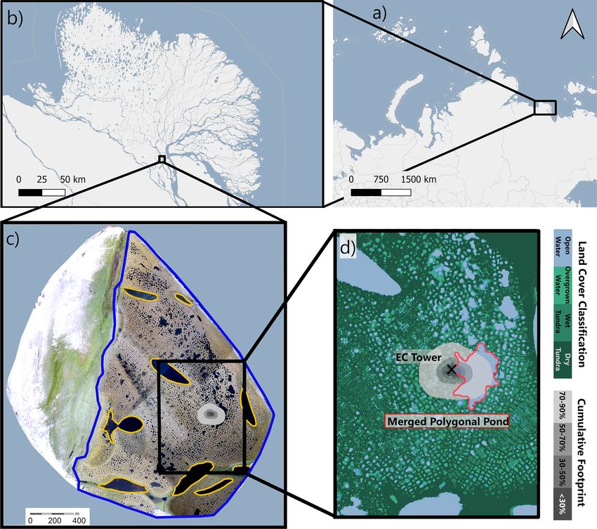
1226                                                        L. Beckebanze, Z. Rehder, et al.: Carbon emissions from ponds

to form, which we term merged polygonal ponds (Rehder                To study spatial and temporal patterns of carbon emis-
et al., 2021). Holgerson and Raymond (2016) as well as Wik        sions from thermokarst ponds, we analyzed land–atmosphere
et al. (2016) report that ponds emit more greenhouse gases        CO2 and CH4 flux observations from an eddy covariance
per unit area than lakes, defined here as water bodies with an    (EC) tower on Samoylov Island, Lena River delta, Russia.
area larger than 8×10⁴ m2 . Thus, in our study area, they have    We set up the EC tower within the polygonal tundra land-
greater potential than lakes to counterbalance the carbon up-     scape at the border between a large merged polygonal pond
take of the surrounding tundra (McGuire et al., 2012; Jammet      and the surrounding semi-terrestrial tundra for 2 months in
et al., 2017; Kuhn et al., 2018). To better understand the im-    summer 2019. The polygonal structures were still clearly
pact of thermokarst ponds on the landscape carbon flux, we        visible along the shore and underwater, and most of the
compare carbon dioxide (CO2 ) and methane (CH4 ) fluxes           pond was shallow (Rehder et al., 2021). Due to the tower’s
from thermokarst ponds to fluxes from the semi-terrestrial        position, fluxes from the merged polygonal pond were the
tundra. The semi-terrestrial tundra consists of wet and dry       dominant source of the observed EC fluxes under easterly
tundra and overgrown shallow water, which are the terrestrial     winds. From other wind directions, the observed EC fluxes
land-surface types used by Muster et al. (2012) to classify       were dominated by semi-terrestrial polygonal tundra with
Samoylov Island.                                                  only a low influence from small polygonal ponds. This pa-
   The main geophysical and biochemical processes that            per aims to deepen the understanding of carbon emissions
drive CH4 fluxes are different to the ones that drive CO2         from thermokarst ponds and constrain their impact on the
fluxes. The microbial decomposition of dissolved organic          landscape carbon balance. We (1) examine the temporal and
carbon, which is introduced laterally into the aquatic system     spatial patterns of net ecosystem exchange (NEE) and the
through rain and meltwater (Neff and Asner, 2001), domi-          spatial pattern of CH4 flux from semi-terrestrial tundra and
nates aquatic CO2 production. When supersaturated with dis-       thermokarst ponds and (2) investigate the influence of the
solved CO2 , ponds emit CO2 into the atmosphere through           thermokarst ponds on the landscape NEE of CO2 during
diffusion. While photosynthetic CO2 uptake has been ob-           the months June to September 2019. To this end, we use a
served in some clear Arctic water bodies (Squires and Le-         footprint model and model NEE of CO2 using the footprint
sack, 2003), most Arctic water bodies are net CO2 sources         weights of semi-terrestrial tundra and thermokarst ponds.
(Kuhn et al., 2018). Estimates of CO2 emissions range from
close to zero (0.028 g m2 d−1 by Treat et al., 2018, and
0.059 g m2 d−1 by Jammet et al., 2017) to substantial (1.4–       2     Methods
2.2 g m2 d−1 by Abnizova et al., 2012).
   Within just one site, CH4 emissions from a water body can      2.1    Study site
vary by up to 5 orders of magnitude: 0.5–6432 mg m2 d−1
(Bouchard et al., 2015). The CH4 that ponds emit is mostly        Samoylov Island (72◦ 220 N, 126◦ 280 E) is located in the
produced in sub-aquatic soils and anoxic bottom waters            southern part of the Lena River delta (Fig. 1b). It is approx-
(Conrad, 1999; Hedderich and Whitman, 2006; Borrel et al.,        imately 5 km2 in size and consists of two geomorphologi-
2011). Additionally, CH4 might also be produced in the            cally different components. The western part of the island
oxic water column (Bogard et al., 2014; Donis et al., 2017),      (∼ 2 km2 ) is a floodplain, which is flooded annually during
though this location of methanogenesis is only significant in     the spring. The eastern part of the island (∼ 3 km2 ), a Late
large water bodies (Günthel et al., 2020). Moreover, there        Holocene river terrace, is characterized by polygonal tun-
is still ongoing debate as to whether methanogenesis oc-          dra. The partially degraded polygonal tundra at this study
curs in oxic waters at all (Encinas Fernández et al., 2016;       site features high spatial heterogeneity on a scale of a few
Peeters et al., 2019). CO2 is also formed as a byproduct          meters in several aspects, including vegetation, water table
of the methanogenesis process (Hedderich and Whitman,             height, and soil properties. Dry and wet vegetated parts of the
2006). Water bodies emit CH4 produced in their benthic zone       semi-terrestrial tundra are interspersed with small and large
through diffusion, ebullition (sudden release of bubbles), or     thermokarst ponds (1 to 10 000 m2 ) and with larger lakes (up
plant-mediated transport. The varying contributions of these      to 0.05 km2 ; Boike et al., 2015a; Kartoziia, 2019). The is-
three local methane emissions pathways lead to high spatial       land is surrounded by the Lena River and sandy floodplains,
variability between water bodies and within a single water        creating additional spatial heterogeneity on a larger scale.
body (Sepulveda-Jauregui et al., 2015; Jansen et al., 2019).         This study focuses on a merged polygonal pond (Figs. 1d
In particular, local seep ebullition causes high spatial vari-    and A1) on the eastern part of the island. This merged polyg-
ance of CH4 emissions within one water body (Walter et al.,       onal pond has a size of 0.024 km2 with a maximum depth of
2006). Variability in the coverage and composition of vascu-      3.4 m and a mean depth of 1.2 m (Rehder et al., 2021; Boike
lar plant communities in a water body can also increase CH4       et al., 2015a). In an aerial image of the pond, the polygonal
variability because CH4 transport efficiency can be species-      structures are clearly visible under the water’s surface (Boike
specific (Knoblauch et al., 2015; Andresen et al., 2017).         et al., 2015c). The vegetated shoreline of this merged polygo-
                                                                  nal pond is dominated by Carex aquatilis, but it also features

Biogeosciences, 19, 1225–1244, 2022                                                   https://doi.org/10.5194/bg-19-1225-2022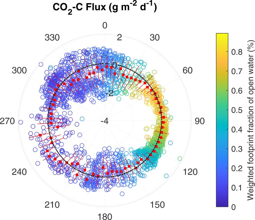
L. Beckebanze, Z. Rehder, et al.: Carbon emissions from ponds                                                                   1227

Carex chordorrhiza, Potentilla palustris, and Aulacomnium            on accurate measurements of the latent and sensible heat flux
spp. These plants grow in the water near the shore, while the        and was applied to the open-path data of the LI-7700. For the
deeper parts of the merged polygonal pond are vegetation-            LI-7700 in particular, the correction term can be larger than
free.                                                                the flux itself, but the correction was derived from the under-
                                                                     lying physical equations. Because we used well-calibrated
2.2   Instruments                                                    instruments as well as EddyPro, which uses an up-to-date
                                                                     implementation of the correction, we were confident that
We measured gas fluxes using an eddy covariance (EC) tower           the LI-7700 would provide accurate CH4 flux estimates. For
between 11 July and 10 September 2019. The EC tower                  enclosed-path data, we performed a sample-by-sample con-
was located on the eastern part of Samoylov Island, di-              version into mixing ratios to account for air-density fluctu-
rectly on the western shore of the merged polygonal pond             ations (Ibrom et al., 2007b; Burba et al., 2012). Flux losses
(Fig. 1d). The EC instruments were mounted on a tripod               occurred in the low- and high-frequency spectral range due to
at a height of 2.25 m (Fig. A1). The tower was equipped              different filtering effects. We compensated for flux losses in
with an enclosed-path CO2 –H2 O sensor (LI-7200, LI-COR              the low-frequency range in accordance with Moncrieff et al.
Biosciences, USA), an open-path CH4 sensor (LI-7700, LI-             (2004) and in the high-frequency range in accordance with
COR Biosciences, USA), and a 3D ultrasonic anemome-                  Fratini et al. (2012). For the high-frequency range compensa-
ter (R3-50, Gill Instruments Limited, UK). All instruments           tion method, a spectral assessment file was created using the
had a sampling rate of 20 Hz. We also installed radiation-           method of Ibrom et al. (2007a). The spectral assessment re-
shielded temperature and humidity sensors at the EC tower            sulted in cutoff frequencies of 3.05 and 1.67 Hz for CO2 and
(HMP155, Vaisala, Finland) and used data from a photosyn-            CH4 , respectively. For H2 O, we found a humidity-dependent
thetically active radiation (PAR) sensor mounted on a tower          cutoff frequency between 1.25 Hz (relative humidity, RH, of
approximately 500 m to the west of the EC tower (SKP 215,            5 %–45 %) and 0.21 Hz (RH 75 %–95 %). We performed a
Skye Instruments, UK). Additional meteorological data for            quality check on each half-hourly flux following the 0–1–2
Samoylov Island were provided by Boike et al. (2019).                system proposed by Mauder and Foken (2004). In this qual-
                                                                     ity check, flux intervals with the lowest quality received the
2.3   Data processing                                                flag “2” and were excluded from further analysis.

We performed the raw data processing and computation of              2.4     Data analysis
half-hourly fluxes for open-path and enclosed-path fluxes
(CO2 , CH4 , and H2 O) using EddyPro 7.0.6 (LI-COR, 2019).           2.4.1    Land-cover classification
The convention of this software is that positive fluxes are
                                                                     The land-cover classification covers the Late Holocene river
fluxes from the surface to the atmosphere, while negative
                                                                     terrace of Samoylov Island (3.0 km2 , area within the blue
fluxes indicate a flux from the atmosphere downwards. Raw
                                                                     line in Fig. 1c). It is based on high-resolution near-infrared
data screening included spike detection and removal accord-
                                                                     (NIR) orthomosaic aerial imagery obtained in the summer of
ing to Vickers and Mahrt (1997) (1 % maximum accepted
                                                                     2008 (Boike et al., 2015b). We used a subset of the existing
spikes and a maximum of three consecutive outliers). Addi-
                                                                     classification of Muster et al. (2012) as a training dataset to
tionally, we applied statistical tests for raw data screening, in-
                                                                     perform semi-supervised land-cover classification using the
cluding tests for amplitude resolution, skewness and kurtosis,
                                                                     maximum likelihood algorithm in ArcMap Version 10.8 (Esri
discontinuities, angle of attack, and horizontal wind steadi-
                                                                     Inc., USA). We then applied the ArcMap majority filter tool
ness. All of these tests’ parameters were set to EddyPro de-
                                                                     to the new classification. The land-cover classification has a
fault values. We rotated the wind-speed axis to a zero-mean
                                                                     resolution of 0.17 m × 0.17 m,. It is projected onto WGS 84
vertical wind speed using the “double rotation” method of
                                                                     UTM Zone 52N, and the land-cover classes include open wa-
Kaimal and Finnigan (1994). Further, we applied linear de-
                                                                     ter (15.7 %), overgrown water (7.0 %), dry tundra (65.1 %),
trending to the raw data following Gash and Culf (1996) be-
                                                                     and wet tundra (12.1 %), as defined by Muster et al. (2012).
fore performing flux calculations. We compensated for time
                                                                     We summarize the classes overgrown water, dry tundra, and
lags via automatic time lag optimization using a time lag as-
                                                                     wet tundra in the land-cover type of semi-terrestrial tundra.
sessment file from a previous EddyPro run. In this previous
                                                                     The river terrace consists of this semi-terrestrial tundra, large
time lag assessment, the time lags for all gases were detected
                                                                     lakes, and thermokarst ponds. Since small ponds are an inte-
using covariance maximization (Fan et al., 1990), resulting
                                                                     gral part of the polygonal tundra, we use the term “polygonal
in time lags between 0 and 0.4 s for CO2 and between −0.5
                                                                     tundra” to refer to the area of the river terrace covered by
and +0.5 s for CH4 . For H2 O, the time lag was humidity-
                                                                     semi-terrestrial tundra and by thermokarst ponds.
dependent and was calculated for 10 humidity classes. We
compensated for air-density fluctuations due to thermal ex-
pansion and contraction and varying water-vapor concentra-
tions, following Webb et al. (1980). This correction depends

https://doi.org/10.5194/bg-19-1225-2022                                                      Biogeosciences, 19, 1225–1244, 2022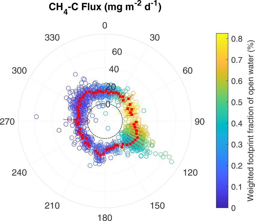
1228                                                              L. Beckebanze, Z. Rehder, et al.: Carbon emissions from ponds

Figure 1. The location of the study site in Russia is shown in (a), and the location of Samoylov Island within the Lena River delta is
shown in (b). Samoylov Island is shown in (c); the surrounding Lena River appears in light blue. The outline of the river terrace land-cover
classification (Sect. 2.4.1) is indicated by the blue line. We focus on the polygonal tundra; however, large lakes are excluded (circled in
yellow). In (d), the land-cover classification is drawn in blue (open water) and green (dark green: dry tundra; medium green: wet tundra; light
green: overgrown water) shades. The merged polygonal pond studied here is outlined in red. The location of the EC tower is marked by a
black cross. The cumulative footprint (see Sect. 2.4.2) is shown in gray shades. Of the flux, 30 % likely originated from within the dark gray
area, 50 % from within the medium dark gray area, 70 % from within the medium light gray area, and 90 % from within the light gray area.
Map data from © OpenStreetMap contributors 2020, distributed under the Open Data Commons Open Database License (ODbL) v1.0 (a, b)
and modified based on Boike et al. (2012) (c, d).

2.4.2   Footprint model                                                   type to each half-hourly flux (from now on referred to as the
                                                                          weighted footprint fraction). The model accounted for the
                                                                          stratification of the atmospheric boundary layer and required
In deploying an EC measurement tower, the tower’s loca-                   a height-independent crosswind distribution and horizontal
tion and sensor height are crucial parameters. A lower mea-               homogeneity of the surface. The input data required station-
surement height results in a smaller footprint. The tower’s               arity of atmospheric conditions during the flux intervals of
footprint describes the source area of the flux within the sur-           30 min.
rounding landscape. As we installed sensors at a height of                   We derived the vertical power-law profiles for the eddy dif-
2.25 m next to the merged polygonal pond, we expected to                  fusivity and the wind speed for each 30 min flux depending
observe substantial flux signals from the adjacent water body             on the atmospheric stratification (see Eq. 6 in Kormann and
as well as from the surrounding semi-terrestrial tundra. Each             Meixner, 2001). We used an analytical approach to find the
land-cover type’s contribution to the flux signal depended on             closest Monin–Obukhov (M–O) similarity profile (see Eq. 36
the wind direction and turbulence characteristics. We imple-              in Kormann and Meixner, 2001). Next, we calculated a two-
mented the analytical footprint model proposed by Kormann                 dimensional probability density function of the source area
and Meixner (2001) in MATLAB (2019). We combined the                      for each flux (from Eqs. 9 and 21 in Kormann and Meixner,
footprint model with land-cover classification data described             2001). We combined each probability density function with
in Sect. 2.4.1 to estimate the contribution of each land-cover

Biogeosciences, 19, 1225–1244, 2022                                                           https://doi.org/10.5194/bg-19-1225-2022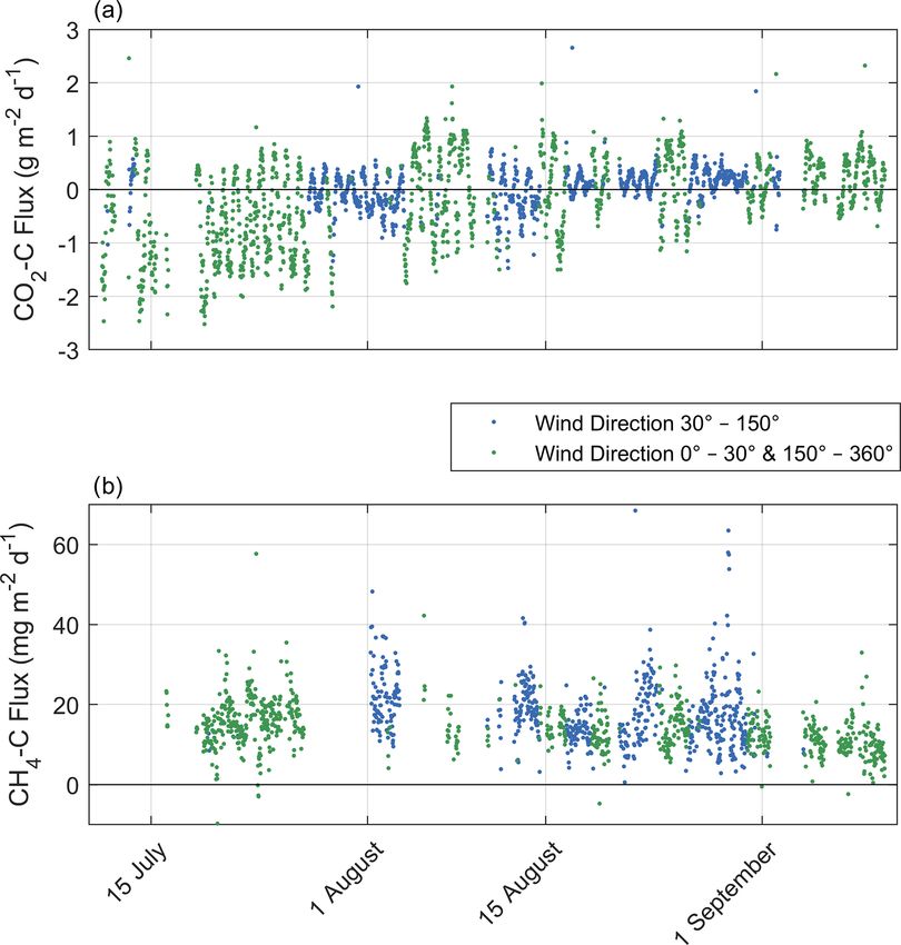
L. Beckebanze, Z. Rehder, et al.: Carbon emissions from ponds                                                                       1229

the land-cover classification of Samoylov Island’s river ter-                 We split the datasets into training (70 %) and validation
race with its four land-cover types (see Sect. 2.4.1). The                (30 %) datasets to test model performance. We implemented
resolution of the footprint model was set to the land-cover               the bulk-NEE model in MATLAB 2019b (MATLAB, 2019)
classification resolution of 0.17 m × 0.17 m. Hence, we were              using the fit function with the NonLinearLeastSquares fit-
able to estimate how much a given grid cell contributed to                ting method. We used the coeffvalues function to estimate
each 30 min flux. We also knew each grid cell’s dominant                  the four parameters (Rbase , Q10 , Pmax , and α) and the confint
land-cover type from the land-cover classification. We com-               function to estimate their 95 % confidence bounds. All par-
bined both pieces of information for each grid cell and cal-              titioned fluxes were converted into CO2 –C fluxes in units of
culated the sum of the fraction fluxes within the source area             g m−2 d−1 before data analysis.
for each of the four land-cover types (dry tundra, wet tundra,
overgrown water, and open water) and determined the con-
                                                                          2.4.4   Separating CO2 fluxes from semi-terrestrial
tribution of each land-cover type with respect to each 30 min
                                                                                  tundra and water bodies
flux (adry tundra , awet tundra , aovergrown water , and aopen water ).
We refer to this contribution of each land-cover type as the
weighted footprint fraction.                                              We wanted to extract fluxes from thermokarst ponds
   We also summed all 30 min two-dimensional probability                  and semi-terrestrial tundra to analyze the influence of
density functions over the entire deployment time. This sum               thermokarst ponds on the carbon balance of a polygonal
is referred to as the cumulative footprint (gray-shaded area in           tundra landscape. However, due to the strong heterogene-
Fig. 1c–d).                                                               ity of the landscape and the relatively small size of the
                                                                          merged polygonal pond compared to the EC footprint, we
2.4.3   Gap-filling the CO2 flux                                          measured a mixed signal from all wind directions. In other
                                                                          words, each flux that was measured with the EC method con-
To gap fill the net ecosystem exchange (NEE) fluxes of CO2 ,              tained information from different land-cover types. We di-
we used the bulk-NEE model proposed by Runkle et al.                      vided the footprint into two classes – semi-terrestrial tundra
(2013). The model is specifically designed to model NEE in                and thermokarst ponds – to assess the impact of thermokarst
Arctic regions: it takes impacts of the polar day into account            ponds on the carbon balance.
by allowing both respiration and photosynthesis to occur si-                 Similar approaches of analyzing heterogeneous eddy co-
multaneously throughout the day. The bulk-NEE model uses                  variance fluxes in Arctic environments have been conducted
the sum of total ecosystem respiration (TER) and gross pri-               for CO2 and CH4 (e.g., Rößger et al., 2019a, b; Tuovinen
mary production (GPP) to describe NEE, our target variable:               et al., 2019). Rößger et al. (2019a, b) extracted CO2 and CH4
NEE = TER + GPP,                                                   (1)    fluxes from two different land-cover classes on a floodplain,
                                                                          while Tuovinen et al. (2019) separated CH4 fluxes from nine
where TER and GPP are in units of           µmol m−2 s−1 .
                                                   TER is
                                                                          individual land-cover classes, including water, and combined
approximated as an exponential function of air temperature
                                                                          them into four source classes (with no separate class for wa-
Tair :
                                                                          ter). All three studies differentiate between fluxes from dif-
                   Tair −Tref
                        γ                                                 ferent vegetation types. Our method is dedicated to distin-
TER = Rbase · Q10               ,                                  (2)    guishing between fluxes from semi-terrestrial tundra and wa-
where Tref = 15 ◦ C and γ = 10 ◦ C are constant, independent              ter bodies.
parameters. Rbase (µmol m−2 s−1 ) describes the basal respi-                 To estimate CO2 fluxes from the merged polygonal pond
ration at the reference temperature Tref , and Q10 (dimension-            (Fpond ), we first fitted the bulk-NEE model to training data,
less) describes the sensitivity of ecosystem respiration to air           excluding fluxes from the direction of the merged polygo-
temperature changes.                                                      nal pond (30◦ < WD < 150◦ , where WD denotes wind direc-
   GPP is described as a rectangular hyperbolic function of               tion). We obtained a dataset consisting of information about
PAR (µmol m−2 s−1 ):                                                      as much semi-terrestrial tundra as possible. We performed
           Pmax · α · PAR                                                 this step since we expected little to no photosynthetic ac-
GPP = −                                                            (3)    tivity in the open-water part of the merged polygonal pond.
           Pmax + α · PAR
                                                                          This gap-filled CO2 flux (hereinafter Fmodeled,mix ) represents
where α (µmol µmol−1 ) is the initial canopy quantum use                  the polygonal tundra surrounding the EC tower, meaning the
efficiency (slope of the fitted curve at PAR = 0) and Pmax                flux is dominated by semi-terrestrial tundra, but also includes
(µmol m−2 s−1 ) is the maximum canopy photosynthetic po-                  polygonal ponds from the wind directions of north, west, and
tential for PAR → ∞.                                                      south. In the model input, we excluded 30 min CO2 fluxes
   The parameters Rbase , Q10 , Pmax , and α were fitted simul-           with an absolute value of more than 4 g m−2 d−1 . In 38 win-
taneously. To account for seasonal changes in plant physi-                dows of 5 d duration, we found an R 2 above 0.9 between the
ology, we fitted the parameters for 5 d running windows as                model output and the validation set. In 18 cases, we obtained
proposed in Holl et al. (2019).                                           an R 2 between 0.8–0.9; in six instances, we obtained an R 2

https://doi.org/10.5194/bg-19-1225-2022                                                          Biogeosciences, 19, 1225–1244, 2022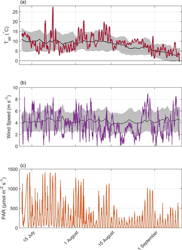
1230                                                           L. Beckebanze, Z. Rehder, et al.: Carbon emissions from ponds

below 0.7. The final RMSE between the model input and the            as we expected different greenhouse gas emission dynam-
gap-filled NEE had a value of 0.29 g m−2 d−1 .                       ics from these lakes and there were no lakes in our footprint
    We assumed that the total observed flux was a linear com-        and therefore within our observation range. Thus, we scaled
bination of the fluxes from the land-cover types weighted            the above numbers to Atundra + Apond = 1, which results in
by their respective contribution to the footprint. Thus, we          Apond = 0.076 and Atundra = 0.924.
postulated that the observed CO2 flux (Fobs,mix , not gap-
filled) was the sum of the individual land-cover type fluxes         2.4.5    CH4 flux partitioning
(Fmodeled,mix and the merged polygonal pond Fpond ) each
multiplied with their weighted footprint fraction (amix and          The data show that the CH4 emissions from the heteroge-
apond ), with aopen water = apond , amix = asum −apond , and asum    neous landscape around the tower were less spatially uniform
being the sum over all land-cover classes:                           than the CO2 emissions. Therefore, we could not use a gap-
                                                                     filling model for CH4 that was similar to the bulk model we
Fobs,mix = apond · Fpond + amix · Fmodeled,mix                       used for CO2 , so we investigated CH4 emissions in a differ-
             Fobs,mix − amix · Fmodeled,mix                          ent way. Based on preliminary results from our analysis and
⇔ Fpond =                                   .                (4)     the aerial image of the study site, we focused on four wind
                         apond
                                                                     sectors instead of extracting the fluxes from the land-cover
To improve data quality, we excluded 30 min fluxes of Fpond          types:
when apond < 50 %. Then, we used the median of Fpond for                 – Tundra. At least half of the footprint consisted of dry
further calculations, and we assumed that all thermokarst                  tundra, and the wind direction was larger than 170◦ .
ponds in the EC footprint emitted the same amount of CO2 .
   As mentioned above, the observed CO2 flux from the wind               – Shore 50◦ (denoted shore50◦ ). Less than 40 % of the
directions of north, west, and south (Fobs,mix ) was influenced            footprint consisted of dry tundra, and water comprised
by polygonal ponds to a small degree. Since our aim was                    at least 30 % of the footprint. The wind direction range
to assess the impact of thermokarst ponds (both polygonal                  was 30◦ < WD < 65◦ .
ponds and merged polygonal ponds) on NEE, we needed to
                                                                         – Pond. At least half of the footprint consisted of open wa-
eliminate the influence of polygonal ponds from our NEE
                                                                           ter, and the wind direction range was 65◦ < WD < 110◦ .
estimate. To extract uncontaminated CO2 flux data from
the semi-terrestrial tundra (Fmodeled,tundra ), we subtracted the        – Shore 120◦ (denoted shore120◦ ). Less than 40 % of the
previously estimated pond CO2 flux Fpond from the observed                 footprint consisted of dry tundra, and water comprised
CO2 flux Fobs,mix :                                                        at least 30 % of the footprint. The wind direction range
                                                                           was 110◦ < WD < 130◦ .
                    Fobs,mix − apond · Fpond
Fmodeled,tundra =                            .               (5)
                              amix                                   2.4.6    CH4 permutation test
We then used this estimated CO2 flux from the semi-                  To evaluate whether the differences in flux medians between
terrestrial tundra Fmodeled,tundra as the regressand variable for    the four wind sectors were significant, we applied a permu-
the bulk-NEE model to obtain a gap-filled dataset regarding          tation test (Edgington and Onghena, 2007). In this test, we
CO2 flux from the semi-terrestrial tundra. This gap-filling          randomly assigned each 30 min flux to one of two groups and
modeling of CO2 –C flux had an RMSE of 0.31 g m−2 d−1 .              calculated both groups’ medians and the differences between
   To evaluate the impact of thermokarst ponds on landscape          the group’s medians. We conducted six tests in total, using
CO2 flux, we estimated a polygonal tundra landscape–CO2              all possible combinations of pairs with the four wind sectors.
flux from the Late Holocene river terrace of Samoylov Is-            After repeating this step 10 000 times, we plotted the result-
land (Flandscape ) by combining thermokarst ponds and semi-          ing differences in medians in a histogram and performed a
terrestrial tundra linearly:                                         one-sample t test to evaluate whether the observed differ-
                                                                     ence in medians differed significantly (p < 0.01) from the
Flandscape = Apond · Fpond + Atundra · Fmodeled,tundra ,
                                                                     randomly generated differences.
where Fpond describes the CO2 emissions from the open-
water areas of thermokarst ponds (Eq. 4), Fmodeled,tundra de-        3     Results
scribes the modeled CO2 flux from the semi-terrestrial tun-
dra (Eq. 5), Apond = 0.07 is the fraction of the river ter-          3.1     Meteorological conditions
race area of Samoylov Island that is covered by thermokarst
ponds (from the land-cover classification; see Sect. 2.4.1),         During the measurement period between 11 July and
and Atundra = 1 − 0.07 is the fraction of the entire river ter-      10 September 2019, half-hourly air temperatures range
race area that consists of other land-cover types. We did not        from −0.5 to 27.6 ◦ C with a mean temperature of 8.7 ◦ C
account for larger or deeper lakes in this upscaling approach        (Fig. A2a). The maximum wind speed measured at the EC

Biogeosciences, 19, 1225–1244, 2022                                                      https://doi.org/10.5194/bg-19-1225-2022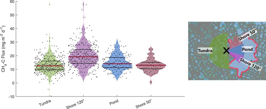
L. Beckebanze, Z. Rehder, et al.: Carbon emissions from ponds                                                                    1231

                                                                      Figure 3. Scatterplot of observed CO2 fluxes against the weighted
                                                                      footprint fraction of open water during each 30 min flux. The air
Figure 2. Polar plot of observed 30 min CO2 –C fluxes with respect    temperature is represented through color. Only fluxes observed in
to the wind direction. Negative values (inside of the dashed black    the nighttime (PAR < 20 µmol m−2 s−1 ) are shown.
line) represent CO2 uptake, while positive values (outside of the
dashed black line) represent CO2 emissions. The values −4, −2,
0, and 2 indicate the magnitude of the CO2 –C flux in g m−2 d−1 .     crease as the pond area contribution increases. Thus, the
The color of each point on the plot represents the percentage the
                                                                      strength of CO2 respiration shows a dependence on the con-
point comprises of the total open-water weighted footprint fraction
                                                                      tribution of open water. We also find that low air temperatures
in each 30 min flux. The red boxes indicate the mean CO2 flux of
5◦ wind direction intervals during the 2-month observation period     are mostly associated with low respiration rates.
(red lines indicate the first standard deviation).                       Another aspect of CO2 flux variability stems from the di-
                                                                      urnal cycle. We compare the diurnal cycle of the CO2 fluxes
                                                                      from the merged polygonal pond (estimated in accordance
tower at a height of 2.25 m is 8.9 m s−1 (Fig. A2b). PAR              with Eq. 4) and the semi-terrestrial tundra (Eq. 5, Fig. 4).
reaches values of up to 1419 µmol m−2 s−1 with decreasing             The results show a less pronounced diurnal CO2 cycle from
maximum values during the measurement period (Fig. A2c).              the direction of the merged polygonal pond (blue) compared
Throughout the measurement period, there are 28 cloudy                to the diurnal CO2 cycle from the semi-terrestrial tundra
days, determined by identifying days with low PAR values              (green). We combine all data from the merged polygonal
(maximum values below ∼ 500 µmol m−2 s−1 ).                           pond (Fpond in Eq. 4), which results in a CO2 –C flux of
                                                                      0.130.24     −2 d−1 (median75th percentile ).
                                                                           0.00 g m               25th percentile
3.2   CO2 fluxes
                                                                      3.3   CH4 fluxes
When inspecting the relation between observed CO2 fluxes
and wind direction (Fig. 2), we find that CO2 fluxes exhibit          We plot the observed CH4 fluxes against wind direction
high temporal variability between positive and negative CO2           (Fig. 5). The results show that the CH4 emissions peak at
fluxes from most wind directions. In the wind sector between          ∼ 120◦ , where fluxes from one shoreline of the merged
60–120◦ , the flux source area is dominated by the merged             polygonal pond contribute to the observed flux (Fig. 1d, from
polygonal pond. The CO2 –C fluxes from this pond sec-                 now on shore120◦ ). We do not observe a similar peak of CH4
tor show smaller absolute variability (0.090.38
                                            −0.33 g m
                                                      −2 d−1 ,
                                                                      emissions in the direction of the second shoreline towards
        95th percentile
median5th percentile ) than the fluxes from all other wind di-        ∼ 50◦ (shore50◦ ). These peaks did not correlate with a specif-
                                             95th percentile          ically large contribution of one of the land-cover classes to
rections (−0.080.87
                 −1.56 g m
                          −2 d−1 , median
                                          5th percentile ). Addi-
tionally, we observe a lower respiration rate from the merged         the footprint.
polygonal pond than from the semi-terrestrial tundra. Fig-               To further investigate the peak at shore120◦ , we com-
ure 3 shows the observed nighttime CO2 fluxes plotted                 pare the CH4 emissions from the different wind sectors
against the respective weighted footprint fraction of open wa-        (shore120◦ , shore50◦ , pond, and tundra; Sect. 2.4.5). We
ter. We define nighttime as having PAR < 20 µmol m−2 s−1 ;            find the following fluxes from the wind sectors: 19.1824.47 14.26
we expect that there would only be respiration and no photo-          (shore120◦ ), 12.9615.11                    18.46
                                                                                          10.34 (shore50 ), 13.9011.02 (pond), and
                                                                                                        ◦

synthesis during the nighttime. We find that the fluxes de-           12.5516.07       −2 d−1 (tundra, median75th percentile ). Fluxes
                                                                            9.65 mg m                          25th percentile

https://doi.org/10.5194/bg-19-1225-2022                                                      Biogeosciences, 19, 1225–1244, 2022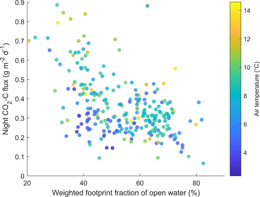
1232                                                            L. Beckebanze, Z. Rehder, et al.: Carbon emissions from ponds

Figure 4. Diurnal cycle of modeled CO2 –C based on observations flux from the merged polygonal pond (blue, Eq. 4) and the semi-terrestrial
tundra (green, Eq. 5) as violin plots for each half-hour flux. Blue and green crosses mark the mean CO2 –C flux during each half-hour flux.
A violin plot shows the distribution of measurements along the y axis – the width of the curves indicates how frequently a certain y value
occurred.

from shore120◦ have a higher median than fluxes from the                   The ratio of CO2 –C to CH4 –C emissions at night
other three wind sectors (Fig. 6).                                      (PAR < 20 µmol m−2 s−1 ) has a value of CH4 / CO2 =
   We investigated the impact of wind speed and air temper-             0.0600.076
                                                                              0.049 for fluxes with an open-water weighted footprint
ature on the CH4 fluxes by excluding flux intervals with high           fraction of more than 60 %, whereas the ratio amounts to
                                                                                                          75th percentile
wind speed (greater than 5 m s−1 ) and high air temperature             CH4 / CO2 = 0.0200.024
                                                                                             0.015 (median25th percentile ) for fluxes with
(warmer than 12 ◦ C). The randomization test (Sect. 2.4.6)              an open-water weighted footprint fraction of less than 20 %.
provided evidence of a significant difference between CH4
emissions from shore120◦ and the other three wind sector                3.4   Upscaled CO2 flux
classes at low wind speeds (top row in Fig. A4) and no signif-
icant difference between the CH4 emissions from the classes             We use the estimated open-water CO2 flux from the merged
pond–tundra and shore50◦ –tundra. The difference between                polygonal pond and the modeled CO2 flux from the semi-
the classes pond and shore50◦ is significant; however, it is            terrestrial tundra to linearly upscale the CO2 flux for the
much smaller than the previously described differences (see             polygonal tundra of Samoylov Island (excluding larger lakes,
central graph in Fig. A4). Note that the CH4 emissions from             the method described in Sect. 2.4.4). As we have not ob-
pond and tundra have a similar magnitude under moderate                 tained estimates for the CH4 fluxes from tundra and pond
wind-speed conditions. The results are very similar for mod-            land-cover types, we only upscale CO2 .
erate temperatures: we find evidence of a significant differ-              We estimate that when one includes the CO2 flux from
ence between the CH4 emissions from shore120◦ and the CH4               thermokarst ponds, the river terrace landscape’s CO2 uptake
emissions from the other three wind sector classes (top row             is ∼ 11 % lower than the uptake of semi-terrestrial tundra
in Fig. A5). The differences in medians between the pond                without ponds. The modeled CO2 –C flux from the semi-
and shore50◦ and between the pond and tundra are signifi-               terrestrial tundra (without consideration of thermokarst pond
cant. However, this difference is much smaller (second row              fluxes) accumulated to −16.29 ± 0.43 g m−2 during the ob-
in Fig. A5). In summary, neither high wind speed nor high               servation period (60.5 d). If separated into months, the mod-
temperatures act as a driver for the high CH4 emissions from            eled CO2 –C flux from the semi-terrestrial tundra amounts
shore120◦ . In contrast, the peak at 180–190◦ can be explained          to −15.01 ± 0.26, −3.56 ± 0.33, and +2.35 ± 0.11 g m−2
reasonably well using air temperature and friction velocity in          in July (19.8 d), August (31 d), and September (9.7 d), re-
multiple linear regression (R 2 = 0.44). Using the same pre-            spectively. When one includes the CO2 flux from the
dictors results in an R 2 of 0.20 for the peak at shore120◦ .           merged polygonal pond to represent all thermokarst ponds
                                                                        on Samoylov Island, the resulting estimate of the land-

Biogeosciences, 19, 1225–1244, 2022                                                         https://doi.org/10.5194/bg-19-1225-2022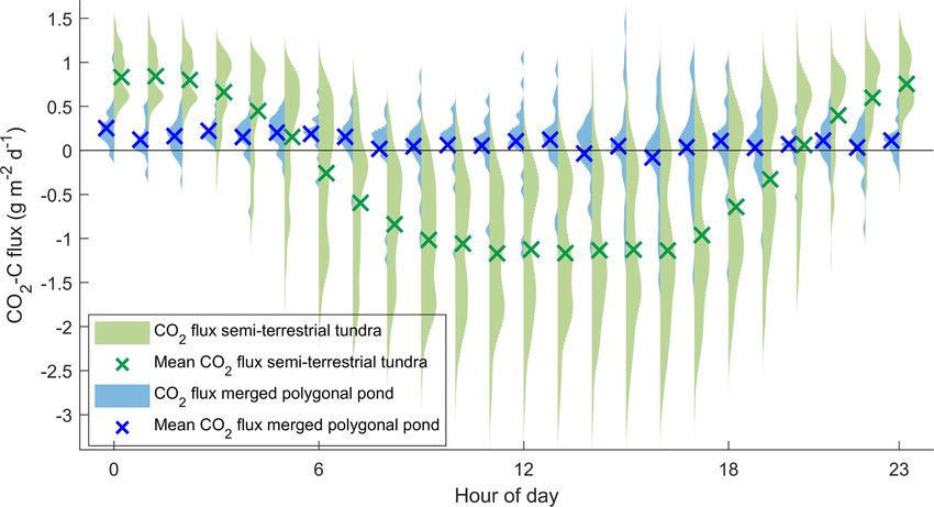
L. Beckebanze, Z. Rehder, et al.: Carbon emissions from ponds                                                                     1233

                                                                       involving multiple lakes in northeast European Russia found
                                                                       that they produce almost zero emissions (0.028 g m−2 d−1 ;
                                                                       Treat et al., 2018).
                                                                          Strikingly, our estimates of open-water CO2 emissions are
                                                                       approximately 12–18 times smaller than those that have been
                                                                       previously reported for open-water CO2 emissions at the
                                                                       same study site (Abnizova et al., 2012). One reason for the di-
                                                                       vergent results might be the different methods used. In Abni-
                                                                       zova et al. (2012), the thin boundary layer (TBL) model, fol-
                                                                       lowing Liss and Slater (1974), was applied to estimate CO2
                                                                       emissions from CO2 concentrations. However, one other
                                                                       study found good agreement between the EC method and the
                                                                       TBL one (Eugster et al., 2003). In addition, in contrast to the
                                                                       larger merged polygonal pond we focus on, Abnizova et al.
                                                                       (2012) measured two polygonal ponds (they took 46 water
                                                                       samples in August and September 2008). These two ponds
                                                                       might have had exceptionally high CO2 concentrations and
                                                                       might not be representative of polygonal ponds in our study
Figure 5. Polar plot of 30 min observed CH4 –C flux with respect       area. If the polygonal ponds in the footprint of our EC mea-
to the wind direction at the EC tower. Positive values outside the     surements emitted CO2 in the quantities suggested by Abni-
dashed black line represent CH4 emissions, while values inside the     zova et al. (2012), we would expect to see their signal more
line represent CH4 uptake during one half-hour period. The val-        clearly in our measurements.
ues 0, 20, 40, and 60 indicate the magnitude of the CH4 –C flux in        Our approach of combining a footprint model with land-
mg m−2 d−1 . The color of each point on the plot represents the per-   cover classification to extract fluxes from different land-
centage the point comprises of the total open-water weighted foot-     cover classes allows us to determine the thermokarst pond
print fraction in each 30 min flux. The red boxes indicate the mean    CO2 flux. We report an uncertainty range with respect to
CH4 flux of 5◦ wind direction intervals during the 2-month obser-      the thermokarst pond CO2 flux; however, identifying the full
vation period (red lines indicate the first standard deviation).
                                                                       uncertainty in this flux is not possible using this approach
                                                                       due to the footprint analysis’ unknown degree of uncertainty.
                                                                       Still, the results with respect to the thermokarst pond CO2
scape CO2 flux amounts to −14.47 ± 0.40 g m−2 (60.5 d),
                                                                       flux are plausible and on the expected order of magnitude
with monthly fluxes of −13.75 ± 0.24, −2.99 ± 0.31, and
                                                                       for two reasons. First, reduced diurnal variability is observed
+2.27 ± 0.10 g m−2 in July (19.8 d), August (31 d), and
                                                                       when the merged polygonal pond influences the flux sig-
September (9.7 d), respectively. Thus, the results show that
                                                                       nal (Fig. 4). This reduction indicates that the respiration rate
thermokarst ponds have the largest impact on the land-
                                                                       from the merged polygonal pond is lower than the respira-
scape’s CO2 flux in August. In September, accounting for
                                                                       tion rate from the semi-terrestrial tundra, where ample oxy-
thermokarst ponds leads to a 3.5 % lower estimate of land-
                                                                       gen is available in the upper soil layer. Additionally, since the
scape CO2 emissions.
                                                                       thermokarst ponds have a lower vegetation density than the
                                                                       tundra, there is less photosynthesis. Second, when focusing
4     Discussion                                                       on nighttime fluxes, when only respiration occurs (i.e., no
                                                                       carbon is taken up), there is a decrease in CO2 emissions
4.1    CO2 flux                                                        with an increasing weighted footprint fraction of open wa-
                                                                       ter (Fig. 3); this also indicates that there is reduced decom-
Only a limited number of EC CO2 flux studies from                      position in the merged polygonal pond. Overall, based on
permafrost-affected ponds and lakes are available (studies             the data, the finding that thermokarst ponds have lower CO2
with “EC” in Table 1). Estimates of open-water EC CO2 –C               emissions than the semi-terrestrial tundra is reasonable.
flux range from 0.059 (Jammet et al., 2017) to 0.11 (Eugster
et al., 2003) to 0.22 g m−2 d−1 (Jonsson et al., 2008). Our es-        4.2   CH4 flux
timate of 0.120.24
                0.0014 g m
                          −2 d−1 is, therefore, well within the

range of open-water CO2 –C fluxes observed with the EC                 We observe large differences in CH4 emissions from the four
method. Other studies using different methods report a wider           wind sectors. CH4 emissions from shore120◦ are significantly
range of open-water CO2 fluxes in Arctic regions. These                higher than from shore50◦ , pond, and tundra (Sect. 3.3). No-
fluxes range from a minor CO2 –C uptake (−0.14 g m−2 d−1 ;             tably, we tested the dependence of these higher fluxes on
Bouchard et al., 2015) to substantial emissions of CO2 –C (up          wind speed and air temperature. We expect high wind speeds
to 2.2 g m−2 d−1 ; Abnizova et al., 2012). A modeling study            to enhance turbulent mixing of the water column and dif-

https://doi.org/10.5194/bg-19-1225-2022                                                       Biogeosciences, 19, 1225–1244, 2022
L. Beckebanze, Z. Rehder, et al.: Carbon emissions from ponds
https://doi.org/10.5194/bg-19-1225-2022
Table 1. Daily mean water–atmosphere CO2 and CH4 fluxes from different study sites. TBL is the abbreviation for thin boundary layer model, EC for eddy covariance, CH for chamber
measurement, MOD for modelled fluxes, STO for storage fluxes, and NEW for the method used in this study. All fluxes are given ± standard deviation, except fluxes from this study are
75th percentile
given as median25th percentile .
CO2 –C flux CH4 –C flux
Study Location Period/time Study site Method (g m−2 d−1 ) (mg m−2 d−1 )
This study Lena River delta, 11 Jul–10 Sep 2019 merged polygonal EC/NEW 0.24
0.130.00 18.67
14.1011.23
northern Siberia pond EC – 15.11 –
12.9610.34
merged polygonal pond 24.47
19.1814.26
shore
Abnizova et al. (2012) Lena River delta, 1 Aug–21 Sep 2008 Samoylov Pond TBL 1.50–2.20 –
northern Siberia Samoylov Lake TBL 1.40–2.10 –
Jammet et al. (2017) Northern Sweden 2012–2013 Villasjön EC 0.059 13.42 ± 1.64
Jonsson et al. (2008) Northern Sweden 17 Jun–15 Oct 2005 Merasjärvi EC 0.22 ± 0.002 –
TBL 0.30 ± 0.01
Eugster et al. (2003) Alaska 27–31 Jul 1995 Toolik Lake EC 0.11 ± 0.033 –
TBL 0.13 ± 0.003
CH 0.37 ± 0.060
Jansen et al. (2019) Northern Sweden Year round, 2010–2017 Villasjön CH 0.22 ± 0.047 14.04 ± 2.25
Inre Harrsjön 0.25 ± 0.05 10.39 ± 1.40
Mellersta Harrsjön 0.73 ± 0.067 13.76 ± 2.81
Bouchard et al. (2015) NE Canada Jul 2013 and 2014 Bylot Island, polygon TBL −0.14–0.74 0.50–6432
ponds −0.085–0.062 0.70–74.5
Lakes
Sepulveda-Jauregui et al. (2015) Alaska Jun–Jul 2011 and 2012 8 lakes, Yedoma TBL & STO 0.60 ± 0.58 92.86 ± 35.72
32 lakes, non-Yedoma 0.10 ± 0.10 16.80 ± 8.61
Biogeosciences, 19, 1225–1244, 2022
Treat et al. (2018) NE European Russia 2006–2015 Multiple lakes MOD 0.028 ± 0.00011 0.84 ± 0.0
Sieczko et al. (2020) Northern Sweden Jul–Aug 2017 Ljusvatterntjärn CH – 2.95 ± 0.75
Ducharme-Riel et al. (2015) NE Canada Summer 2008 15 lakes TBL 0.20 ± 0.093 –
Repo et al. (2007) Western Siberia 3 Jul–6 Sep 2005 MTlake TBL 0.14 ± 0.11 –
FTlake TBL 0.41 ± 0.25
MTpond TBL 0.44 ± 0.25
Lundin et al. (2013) Northern Sweden 2009 (only ice-free sea- 27 lakes TBL 0.18 ± 0.11 –
son)
Kling et al. (1992) Alaska 1975–1989 25 lakes TBL 0.25 ± 0.040 5.16 ± 0.96
1234L. Beckebanze, Z. Rehder, et al.: Carbon emissions from ponds 1235 Figure 6. Violin plots of observed CH4 emissions at the EC tower separated into four different wind sector classes. A violin plot shows the distribution of measurements along the y axis – the width of the shapes indicates how frequently a certain y value occurred. Medians of CH4 emission distributions are shown as red lines, and 75th and 25th percentile are shown as black lines. On the right, the wind sectors with the eddy covariance tower in the center (black cross) are shown. fusive CH4 outgassing at the water–atmosphere interface. resolution > 0.33 m) show no signs of erosion. We therefore High wind speeds are also associated with pressure pump- assume that past erosion is unlikely is unlikely to have been ing, which potentially fosters the ebullition of CH4 . On the a factor that caused the high levels of CH4 emissions we ob- other hand, peak temperatures can lead to peak CH4 pro- served in 2019. duction and emissions due to enhanced biological activity. Local ebullition of the merged polygonal pond could However, the high emissions from shore120◦ do not coincide lead to high CH4 emissions from shore120◦ . We applied the with either of two key meteorological conditions, high wind method proposed by Iwata et al. (2018) to check for signs of speeds and high temperatures, which would especially favor ebullition events. This method uses the 20 Hz raw CH4 con- high emissions. Thus, the difference in methane flux dynam- centration data to detect short-term peaks in CH4 that origi- ics between shore120◦ and shore50◦ is astounding since the nate from ebullition events. However, we cannot detect ebul- shorelines share many other characteristics. lition events in the 20 Hz raw data. Both shorelines extend radially (in a fairly straight line) In summary, meteorological conditions (wind speed and from the EC tower (Fig. 1), thus contributing similarly to the temperature), characteristics of emergent vegetation, coastal EC flux. The underwater topography does not vary signif- erosion, and intense ebullition events are unlikely to be the icantly between the two shorelines. Meters away from the main driving factors of the increased CH4 emissions we ob- shore, both shorelines have a water depth of a few cen- served. Another possible driver of higher CH4 emissions timeters and a few decimeters (see data from Boike et al., from shore120◦ is a small but steady seep ebullition hot spot 2015a). As previously described in Sect. 2.1, both shore- close to this shoreline (such as ebullition class kotenok in lines are dominated by Carex aquatilis, and from visual in- Walter et al., 2006). Seep ebullition hot spots have been re- spection, we could not identify differences in shoot density. ported to occur heterogeneously in clusters in Alaskan lakes We, therefore, assume that the characteristics of the emer- (Walter Anthony and Anthony, 2013). Unfortunately, seep gent vegetation do not play a major role in explaining the ebullition has not previously been reported in water bodies differences between the CH4 emissions from shore120◦ and in our study area, so we did not include measurements tar- shore50◦ . We also examine the evolution of the shorelines at geting this process in our measurement campaign. In future the merged polygonal pond to check whether erosion along studies, visual inspection of trapped CH4 bubbles in the ice the shoreline could cause the high CH4 emissions. We com- column during wintertime, as proposed by Vonk et al. (2015), pare an image from 1965 ( Earth Resources Observation and could reveal more information about the cause of the higher Science , EROS) with the current (2019) shoreline, yet we CH4 emissions from shore120◦ , as could funnel or chamber cannot identify signs of recent erosion. Furthermore, high- measurements with high spatial coverage. resolution aerial images of this pond from 2008 (Boike et al., The results show that the merged polygonal pond emits 2015b, resolution > 0.33 m) and 2015 (Boike et al., 2015c, a similar magnitude of CH4 to the polygonal tundra surface https://doi.org/10.5194/bg-19-1225-2022 Biogeosciences, 19, 1225–1244, 2022
1236                                                       L. Beckebanze, Z. Rehder, et al.: Carbon emissions from ponds

under similar meteorological conditions and when exclud-         4.3    Upscaling the CO2 flux
ing the high emissions from shore120◦ . However, substrate
availability and temperature dynamics differ substantially.      We upscale the CO2 emissions for the river terrace on
Additionally, in dense soils, methane diffuses slowly enough     Samoylov, an area for which we have access to high-
through soil layers containing oxygen for the methane to be      resolution land-cover classification. We find that we over-
oxidized before reaching the surface. In contrast, methane       estimate the carbon dioxide uptake of the polygonal tundra
emitted in ponds can reach the surface quickly through ebul-     by 11 % when we do not account for the thermokarst ponds’
lition or plant-mediated transport in addition to diffusion.     CO2 emissions. A similar approach by Abnizova et al. (2012)
Therefore, we expect to see larger differences between the       found a potential increase of 35 %–62 % in the estimate of
CH4 emissions from the merged polygonal pond and the             CO2 emissions from the Lena River delta when including
polygonal tundra, more akin to the differences that have been    small ponds and lakes in the landscape CO2 emission calcu-
detected in a subarctic lake and fen by Jammet et al. (2017).    lation. If we were to follow the upscaling approach by Abni-
However, we see no significant difference in the CH4 emis-       zova et al. (2012) and consider overgrown water as part of the
sions from the open-water areas of the merged polygonal          thermokarst ponds, the estimate of the landscape CO2 uptake
pond and the polygonal tundra surface (Figs. 6 and A4).          would decrease by 19 %. Kuhn et al. (2018) also found wa-
    Since many other thermokarst ponds in our study area are     ter bodies in Arctic regions to be an important source of car-
smaller than the merged polygonal pond (making them un-          bon, which could outbalance the carbon dioxide uptake of the
suitable to study using the EC method) and since smaller         semi-terrestrial tundra in a future climate. In summary, our
ponds tend to be greater emitters of methane (Holgerson and      results demonstrate that open-water CO2 emissions can sub-
Raymond, 2016; Wik et al., 2016), our measurements might         stantially influence the summer carbon balance of the polyg-
provide a lower limit of overall thermokarst pond CH4 emis-      onal tundra. With respect to the night time emissions, we find
sions.                                                           that per gram CO2 –C thermokarst ponds emit 0.06 g CH4 –C
    We estimate a CH4 –C flux of 13.3815.92  10.55 mg m
                                                       −2 d−1    whereas the semi-terrestrial tundra only emits 0.02 g CH4 –
         75th percentile
(median25th percentile ) from the merged polygonal pond          C. This finding underlines again that, especially when con-
                                                                 sidering thermokarst ponds, CH4 emissions are of significant
and 12.9615.11           24.47
            10.34 –19.1814.26 mg m
                                  −2 d−1 from the shores of
                                                                 interest. Even though mean CH4 emissions from the semi-
this pond. This is higher than the fluxes measured
                                                                 terrestrial tundra and open water are of similar magnitude,
by Jammet et al. (2017) from a subarctic lake (Ta-
                                                                 we expect that the impact of thermokarst ponds on the car-
ble 1). The authors report a mean annual CH4 –C flux of
                                                                 bon balance would be even greater when accounting for CH4
13.42 ± 1.64 mg m−2 d−1 and a mean ice-free-season CH4 –
                                                                 due to locally high emissions.
C flux of 7.58 ± 0.69 mg m−2 d−1 . A study focusing on
                                                                    Our results suggest that future studies that aim to cap-
32 non-Yedoma thermokarst lakes in Alaska found CH4 –C
                                                                 ture a representative landscape flux should pay extra atten-
emissions similar to our results (16.80 ± 8.61 mg m−2 d−1 ;
                                                                 tion to the water bodies in their footprint. The CO2 flux from
Sepulveda-Jauregui et al., 2015). Also, a synthesis of
                                                                 thermokarst ponds has the opposite sign (CO2 emissions) to
149 thermokarst water bodies north of ∼ 50◦ N re-
                                                                 the semi-terrestrial tundra (CO2 uptake) during the observa-
ports CH4 –C emissions on the same order of magnitude
                                                                 tion period. Consequently, thermokarst ponds should cover
(27.57 ± 14.77 mg m−2 d−1 ; Wik et al., 2016). However,
                                                                 about as much area in the measurement as they do in the
other recent studies have reported considerably lower CH4 –
                                                                 landscape area of interest. In this way, the chances of captur-
C emissions of 2.95 ± 0.75 mg m−2 d−1 in northern Swe-
                                                                 ing CH4 hot spots, which can be investigated more closely,
den (Sieczko et al., 2020), and, in contrast, a study found
                                                                 are also greater.
CH4 –C emissions of up to 6432 mg m−2 d−1 in northeast
Canada (Bouchard et al., 2015). The wide range of water-
body methane emissions militates in favor of caution when
generalizing our results, even for Samoylov Island, espe-        5     Conclusions
cially since the emissions within the merged polygonal pond
                                                                 We find that thermokarst ponds are a carbon source. At the
have been shown to be heterogeneous. Instead, after finding a
                                                                 same time, the surrounding semi-terrestrial tundra in our
hot spot in CH4 emissions at the pond shore, we would like to
                                                                 study area acts as a carbon sink during the summer period
highlight that the gathering of additional measurements – for
                                                                 (July–September), which is in agreement with prior studies
example employing funnel traps or counting bubbles in ice –
                                                                 (Abnizova et al., 2012; Jammet et al., 2017), despite us ob-
will help to better constrain thermokarst pond CH4 dynam-
                                                                 serving much lower open-water CO2 fluxes compared to pre-
ics in their full complexity. Nevertheless, our measurements
                                                                 vious work at the same study site (Abnizova et al., 2012).
provide a robust lower limit of thermokarst pond CH4 emis-
                                                                 Using our approach to disentangle the EC fluxes from differ-
sions.
                                                                 ent land-cover classes, we posit that during the measurement
                                                                 period, we would overestimate the carbon dioxide uptake of
                                                                 the polygonal tundra by 11 % if thermokarst ponds were not

Biogeosciences, 19, 1225–1244, 2022                                                  https://doi.org/10.5194/bg-19-1225-2022
L. Beckebanze, Z. Rehder, et al.: Carbon emissions from ponds 1237 accounted for. We expect lakes to have a similar effect on the carbon budget, though a smaller one, since lakes (a) cover a similar amount of surface area as the thermokarst ponds in our study site (Abnizova et al., 2012; Muster et al., 2012) and (b) are weaker emitters of greenhouse gases than ponds (Holgerson and Raymond, 2016; Wik et al., 2016). In contrast to CO2 emissions, which are spatially more homogeneous, small-scale heterogeneity in CH4 emissions makes it difficult to find drivers of CH4 emissions. We cannot pinpoint the drivers behind the high emissions along parts of the coastline, which we surmise were potentially caused by seep ebullition. Thus, we cannot estimate the impact of this heterogeneity on the landscape scale and, therefore, refrain from upscaling CH4 emissions. Additionally, the open-water fluxes presented in this paper originate from a single merged polygonal pond since the other polygonal ponds surrounding the EC tower are too small to extract their fluxes using the footprint method applied here. Thus, we do not account for the spatial variability in CH4 emissions between thermokarst ponds, which can be substantial (Rehder et al., 2021; Wik et al., 2016). However, we note that open-water fluxes were of a similar magnitude to the polygonal tundra fluxes. Conse- quently, the main impact that thermokarst ponds have on the landscape CH4 budget might occur through plant-mediated transport and local ebullition. While being ill-suited for the study of smaller ponds, we underline that the EC method is appropriate for observing greenhouse gas fluxes from thermokarst ponds as small as 0.024 km2 . The EC method has a higher temporal resolution than the TBL method. It does not disturb exchange processes like the chamber flux method, which eliminates the wind at the water surface. Especially when combining an EC foot- print with land-cover classification, one can distinguish be- tween the contribution of different land-cover classes effec- tively and also study the fluxes from thermokarst ponds. We conclude that thermokarst ponds contribute signifi- cantly to the landscape carbon budget. Changes in Arctic hydrology and the concomitant changes in the water-body distribution in permafrost landscapes may cause these land- scapes to change from being overall carbon sinks to overall carbon sources. https://doi.org/10.5194/bg-19-1225-2022 Biogeosciences, 19, 1225–1244, 2022
You can also read