Household Disaggregation and Template Models

Household Disaggregation and Template Models

                      Thomas Rutherford, Andrew Schreiber

                                    April 23, 2021

The views expressed in this presentation are those of the author(s) and do not necessarily
represent the views or policies of the EPA or the University of Wisconsin-Madison.

Outline

1 Overview

2 Calibration Routine

3 Modeling Applications

Introduction

- First version of WiNDC featured a state level dataset with a single
  representative agent by region.
- Provided means for spatially denominated distributional analysis, but
  not within consumer types.
- A key advantage of IMPLAN was its disaggregation of regional
  consumer demands and incomes by household income groups.
- Many ways to go about this type of disaggregation. Incomes vs.
  expenditures.

    - We approach this problem from the income side. Key challenges:
      denominate reasonable transfer income, understand income tax
      liabilities, savings, capital ownership vs. demands, salaries and
      wages.
    - Additional wrinkle: static vs. steady state calibration.
    - Income elasticities used to separate household level commodity
      expenditures.

What We Do

Recalibration routine:

  - Two versions of a household dataset is produced. One primarily based
    on the Current Population Survey (CPS), and the other based primarily
    on IRS’s Statistics of Income (SOI).
  - Both versions use a bit of information from the other. Transfers and
    capital gains.
  - Roughly comparable with 5 household types by region. Households vs.
    returns.

Modeling applications:

  - Static vs. steady state static vs. transition dynamic models.
  - Marginal cost of funds.
  - Energy tax example – base dataset vs. blueNOTE.
  - Impacts of COVID.

Table of Contents

1 Overview

2 Calibration Routine

3 Modeling Applications

Income Balance in the Benchmark Equilibrium

Original regional representation (subscripted by r ) – limited by information
in the reference input output tables:

               consr + invr = wagesr + capr + otherr     ∀ r

  - Investment based on location of state level investment demands. May
    not follow location of entity actually doing the investing.
  - Wages and capital income based on sectors in a given state doing the
    demanding. Again, same issue. Furthermore, they are gross of taxes.
  - Other is a closure parameter – all the stuff that can’t be explained by
    consumption, investment, wages and capital.

Obvious issues when thinking about welfare impacts.

Toward a Better Income Balance Representation
While regional representation may limit ability to do reasonable welfare
analysis, it does provide useful control totals that are consistent with both
the National Income and Product Accounts (NIPA) and accounting
identities for the rest of the economy.

This work seeks to reconcile the issues outlined in the previous slide. Move
toward the following income balance representation:
        consrh + taxrh + saverh = wagesrh + caprh + trnrh    ∀ (r , h)
  - Break out each category by region and household income type (h).
  - Estimate savings for household-region pairs investing in new capital.
  - Estimate wage and extant capital endowments consistent with where
    people actual live and work. Incorporate income taxes into WiNDC
    structure.
  - Break out the “other” category into cash payment transfers consistent
    with benefits programs in US. Assume all transfers are between
    households and government. No intra-household transfers assumed
    here.

Datasets Used in Disaggregation

Households vs. Number of Returns

In what follows, we aggregate households into 5 groups that roughly
correspond with one another. Comparison between two datasets not perfect.

Households vs. Number of Returns

CPS Categories (2016)

CPS: National Level Shares (2016)

CPS: State Level Observation Count (2016)

CPS Literature on Underreporting

There is a healthy literature assessing CPS underreporting. Two papers that
are particularly useful here:

  - Meyers et al. (2009): compares CPS transfer data to administrative
    totals and reports share of total.
  - Rothbaum (2015): compares CPS data to NIPA accounts and reports
    share of total for transfers not in Meyers et al. (2009) and capital
    income.

Tax Rates for CPS-based Dataset
The CPS does not include tax payments. We estimate average and marginal
tax rates with CPS data and TAXSIM (v27) based on Alex Marten’s code
base in the SAGE model package (see: https://www.epa.gov/
environmental-economics/cge-modeling-regulatory-analysis).

SOI Categories (2016)

Comparison of Labor Income Taxes

While tax payments are endogenized in the routine, tax rates are held fixed.

  - Overall income tax rates calculated directly from data for SOI
    recalibration. Labor income taxes net out taxes paid on capital income.
  - CPS based taxes from TAXSIM.

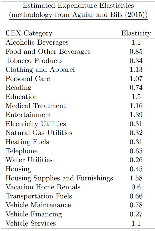
Average labor income tax rates by household are computed as:

Expenditure Side
Household expenditures differentiated by income group is based on expenditure
elasticities from the SAGE model that were estimated using data from the
Consumer Expenditure Survey. Mapped to WiNDC sectors using the PCE Bridge.

Structure of Recalibration Routine

The recalibration routine is run for data from 2015-2017 based on either the
SOI or CPS income data. Some synergy between the two to get them
roughly lined up.

  - CPS based recalibration: augmented with SOI capital gains.
  - SOI based recalibration: augmented with CPS transfer totals. SOI
    transfer data is insufficient for us because it is only taxable transfers.
    Most cash payment benefits aren’t taxed.

Structure of Recalibration Routine

4 step process:

 1. Solve for steady state equilibrium investment demands (if option is
    selected – static vs. steadystate).

       - Important because investment levels tie directly to the income
         balance constraint for households in the form of savings.
         Considering this upfront circumvents issues down the line.

 2. Solve income routine for aggregated regions (here Census regions).
 3. Solve income routine at the state level enforcing control totals at the
    aggregated region level.
 4. Solve expenditure routine at the state level.

Successive calibration enhances reliability when solving larger model.

Step 1: Steady State Recalibration

A steady state equilibrium requires that investment and capital demands
have the following relationship:
                    X             X (gr + δ)
                         i0rg =              kd0rs   ∀   r
                     g            s
                                    (ir + δ)

Using gross capital demands, reference investment is scaled by a lot (≈2x).

We impose a capital tax rate taken from SAGE (33%), which is inclusive of
corporate and income taxes on capital. Using net capital demands,
reference investment is scaled by ≈1.4x.

Note that we also recalibrate other commodity parameters to accommodate
changes in i0rg (production, intermediate demand, regional demand).

Step 2: Income (Aggregated Regions)
Objective: minimize the deviation from either CPS or SOI data.

Key highlights:

  - Assumptions on wages:

       - Labor markets clear within census regions
       - Labor demands account for overhead outside of what employees
         get paid directly for wages and salary. Fringe benefits are shared
         evenly across household types

  - Note that wages, interest payments, transfers, consumption and taxes
    are all well controlled. Savings is calculated as a residual of the income
    balance condition which also determines foreign savings.
  - hh5 has much larger totals than what is in the CPS. In part due to
    top-coding in the survey data and smaller capital payments in CPS
    data.
  - Matches literature well on small savings for poorer households (e.g.
    Zucman and Saez type work).

Step 3: Income (State Level)

Key difference to aggregated region routine:

  - Labor market characterization

       - some people live and work in different states (e.g. for DC and AK)

    Key innovation – adding a subscript to match the data well. e.g.

    Given successive recalibration, implicitly assume that labor markets
    clear at the Census region level.

Step 4: Goods Expenditures (State Level)

Examples results:

Additional Thoughts

- Adding income bins would likely need some more work assessing
  representativeness of underlying survey data.
- Data on fringe benefit allocation.
- Jury’s still out about how in-kind benefits are incorporated into input
  output tables.
- Comparison to IMPLAN. Will bring this work back given the finalized
  household build.

Table of Contents

1 Overview

2 Calibration Routine

3 Modeling Applications

Developed Models and Applications

Models:

1. Static model with labor-leisure choice.
2. Steady state static framework relying on Tobin’s Q assumption.
3. Transition intertemporal model differentiating between households that
   can save and those that cannot.

Applications:

  - Marginal Cost of Funds [1,2].
  - Energy taxes using both a base dataset and blueNOTE dataset [1].
  - COVID (requires augmenting dataset with occupations from BLS) [3].

Diagnostic Simulation #1: the MCF

Initial calculation to discuss the welfare cost of tax instruments. Includes:

  - the capital tax (TK ), the labor tax (TL), indirect taxes on production
    (TY ), sales and property taxes (TA) and the import tariff (TM).

Marginal Cost of Funds is computed as the change in equivalent variation
relative to the change in increases in government income as a result of
increases in the tax rate.

While not shown here, also consider alternative social welfare functions in
this calculation with multiple households. Reporting changes in welfare by
summing across households implicitly assumes utilitarian framework.

Marginal Cost of Funds

CPS versus SOI and Static versus Steadystate

Diagnostic Simulation # 2: the Double Dividend
Fullerton & Metcalf (1997): “Environmental Taxes and the Double-Dividend
Hypothesis: Did You Really Expect Something for Nothing?”

The double-dividend hypothesis’ suggests that increased taxes on polluting
activities can provide two kinds of benefits:

 1. improvement in the environment
 2. improvement in economic efficiency from the use of environmental tax
    revenues to reduce other taxes such as income taxes that distort labor
    supply and saving decisions.

Application:

  - construct a minimal energy-economy model with KLEM structure and
    fixed factor resource supply.
  - impose an ad-valorem tax on oil, natural gas and coal of 50%.
  - simulate differences between base dataset and one recalibrated to
    SEDS using new version of blueNOTE.

Economic Cost of Energy Tax (%)

N.B.! Revenue recycled proportional to existing household transfers.

Diagnostic Simulation # 3: COVID

COVID has produced a reduction in the labor demanded by many sectors in
the economy, particularly those with limited telework.

Application:

  - use an intertemporal transition model to understand long run
    implications of a labor demand shock.
  - integrate data from BLS on occupations to model jobs hit hardest by
    the pandemic, typically those in lower income households.
  - simulate differences between a model with no occupations with one
    with the margin explicitly denominated.

Models are formulated by results TBD.

Thanks for listening!

Please email us with any questions that you might have:

              schreiber.andrew@epa.gov
               rutherford@aae.wisc.edu