High-resolution land use and land cover dataset for regional climate modelling: a plant functional type map for Europe 2015
←
→
Page content transcription
If your browser does not render page correctly, please read the page content below
Earth Syst. Sci. Data, 14, 1735–1794, 2022
https://doi.org/10.5194/essd-14-1735-2022
© Author(s) 2022. This work is distributed under
the Creative Commons Attribution 4.0 License.

            High-resolution land use and land cover dataset for
               regional climate modelling: a plant functional
                         type map for Europe 2015
          Vanessa Reinhart1,2 , Peter Hoffmann1,2 , Diana Rechid1 , Jürgen Böhner2 , and Benjamin Bechtel3
                        1 Climate  Service Center Germany (GERICS), Helmholtz-Zentrum Hereon,
                                          Fischertwiete 1, 20095 Hamburg, Germany
         2 Institute of Geography, Section Physical Geography, Center for Earth System Research and Sustainability

          (CEN), Cluster of Excellence “Climate, Climatic Change, and Society” (CLICCS), Universität Hamburg,
                                         Bundesstraße 55, 20146 Hamburg, Germany
                  3 Department of Geography, Ruhr-Universität Bochum, Universitätsstraße 150/Gebäude IA,

                                                  44801 Bochum, Germany
                            Correspondence: Vanessa Reinhart (vanessa.reinhart@hereon.de)

                                   Received: 23 July 2021 – Discussion started: 10 August 2021
                           Revised: 1 March 2022 – Accepted: 1 March 2022 – Published: 13 April 2022

      Abstract. The concept of plant functional types (PFTs) is shown to be beneficial in representing the com-
      plexity of plant characteristics in land use and climate change studies using regional climate models (RCMs).
      By representing land use and land cover (LULC) as functional traits, responses and effects of specific plant
      communities can be directly coupled to the lowest atmospheric layers. To meet the requirements of RCMs
      for realistic LULC distribution, we developed a PFT dataset for Europe (LANDMATE PFT Version 1.0; http:
      //doi.org/10.26050/WDCC/LM_PFT_LandCov_EUR2015_v1.0, Reinhart et al., 2021b). The dataset is based on
      the high-resolution European Space Agency Climate Change Initiative (ESA-CCI) land cover dataset and is
      further improved through the additional use of climate information. Within the LANDMATE – LAND surface
      Modifications and its feedbacks on local and regional cliMATE – PFT dataset, satellite-based LULC information
      and climate data are combined to create the representation of the diverse plant communities and their functions in
      the respective regional ecosystems while keeping the dataset most flexible for application in RCMs. Each LULC
      class of ESA-CCI is translated into PFT or PFT fractions including climate information by using the Holdridge
      life zone concept. Through consideration of regional climate data, the resulting PFT map for Europe is region-
      ally customized. A thorough evaluation of the LANDMATE PFT dataset is done using a comprehensive ground
      truth database over the European continent. The assessment shows that the dominant LULC types, cropland and
      woodland, are well represented within the dataset, while uncertainties are found for some less represented LULC
      types. The LANDMATE PFT dataset provides a realistic, high-resolution LULC distribution for implementation
      in RCMs and is used as a basis for the Land Use and Climate Across Scales (LUCAS) Land Use Change (LUC)
      dataset which is available for use as LULC change input for RCM experiment set-ups focused on investigating
      LULC change impact.

Published by Copernicus Publications.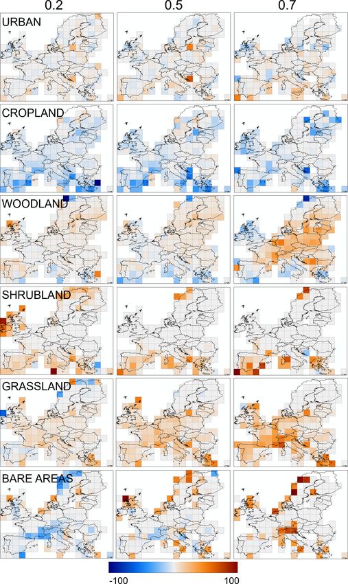
1736                                                              V. Reinhart et al.: The LANDMATE PFT map for Europe 2015

1   Introduction                                                     senting the biosphere was discussed by Lavorel et al. (2007).
                                                                     One criterion that is highly emphasized is the inter-regional
Land use and land cover (LULC), including the vegetation             applicability of a preferably simple PFT classification, which
type and function, were declared essential climate variables         has the ability to capture key characteristics of the biosphere
(ECVs) by the Global Climate Observing System (GCOS)                 from biome to continental scale, regardless of climate zone
(Bojinski et al., 2014). Changes in ECVs are crucial factors         and individual vegetation composition. A variety of PFT
of climate change and therefore need to be monitored and             definitions and cross-walking procedures (CWPs), used for
further represented in climate models to be able to assimi-          translating LULC products into global or regional PFT maps,
late and understand atmospheric processes and feedback ef-           emerged in the last decades (Bonan et al., 2002; Poulter et al.,
fects on different scales. For LULC, anthropogenic modifi-           2011; Ottlé et al., 2013; Poulter et al., 2015). The respective
cations are the most important drivers of change. Deforesta-         CWP documentation consists of the utilized input data, the
tion and reforestation and expansion of urban and cropland           translation table where each LULC class is assigned to PFT
areas affect biogeophysical (e.g. albedo, roughness, evapo-          proportions and a description of how the input data are used
transpiration, runoff) and biogeochemical (e.g. carbon emis-         to create the final product. However, the individual PFT defi-
sions and sinks) surface properties and processes (Mahmood           nitions and CWPs as well as the mostly satellite-based input
et al., 2014; Lawrence and Vandecar, 2015; Alkama and                data differ greatly in complexity and temporal and horizontal
Cescatti, 2016; Perugini et al., 2017; Davin et al., 2020). Be-      resolution (Bonan et al., 2002; Winter et al., 2009; Lu and
sides LULC changes, land management practices are being              Kueppers, 2012). Moreover, inter-regional consistency can-
assessed regarding the influence of related land surface mod-        not be achieved by products that originate from regionally
ifications on regional climate and also the potential of land        constrained input data or regionally adapted CWPs. There-
management practices regarding climate change adaptation             fore, the additional use of climate information in the CWP
and mitigation efforts (Lobell et al., 2006; Kueppers et al.,        from LULC to PFT is a highly useful step in order to create
2007; Burke and Emerick, 2016).                                      a dynamically customizable product that can be adapted to
   In order to represent impacts and feedbacks of LULC               various climate and vegetation characteristics (Poulter et al.,
modifications as realistically as possible, regional climate         2011).
models (RCMs) require an accurate representation of LULC                With the present work, we introduce a PFT map for the
and its changes. In this context, the concept of plant func-         European continent that specifically addresses the require-
tional types (PFTs) is used frequently for the representation        ments of the RCM community. The land cover maps of the
of LULC in RCMs (Davin et al., 2020).                                European Space Agency Climate Change Initiative (ESA-
   PFTs are aggregated plant species groups that share com-          CCI) are translated into 16 PFTs, creating an updated ver-
parable biophysical properties and functions. The aggrega-           sion of the interactive MOsaic-based Vegetation (iMOVE)
tion makes it possible to represent these functionality groups       PFTs that were originally developed for the RCM REMO
within one single model grid unit as a mosaic. The main dif-         (Wilhelm et al., 2014). Climate information is implemented
ference of the PFT representation in comparison to the LULC          in the CWP by employing the Holdridge ecosystem classi-
class representation is the grouping of vegetation according         fication concept based on the Holdridge life zones (HLZs;
to function instead of a descriptive definition. The function        Holdridge, 1967), which provide a global classification of
of a group is directly represented by the biophysical and bio-       climatic zones in relation to potential vegetation cover. The
chemical properties that are prescribed or dynamically com-          HLZ concept is commonly used as a tool for ecosystem
puted within the vegetation layer of an RCM. A comprehen-            mapping from various overlapping research communities
sive review of the subsequent development of PFTs repre-             (Lugo et al., 1999; Yue et al., 2001; Khatun et al., 2013;
senting vegetation dynamics in climate models was done by            Szelepcsényi et al., 2014; Tatli and Dalfes, 2021). This pa-
Wullschleger et al. (2014). Attempts have been made, partic-         per gives detailed documentation on the preparation of the
ularly by the dynamic global vegetation modelling commu-             PFT map – hereinafter referred to as “LANDMATE PFT” –
nity, to move beyond the PFT representation and apply the            within the Helmholtz Institute for Climate Service Science
concept of plant functional traits (e.g. van Bodegom et al.,         (HICSS) project “Modelling human LAND surface Modifi-
2014; Yang et al., 2015). While some plant functional traits         cations and its feedbacks on local and regional cliMATE”
are already introduced to land surface models, which are em-         (LANDMATE). The LANDMATE PFT map is prepared in
ployed by RCMs (e.g. Li et al., 2021), there is debate whether       close collaboration with the EURO-CORDEX Flagship Pi-
the PFT approach can be replaced by the plant functional             lot Study Land Use and Climate Across Scales (FPS LU-
traits approach or by using new evolution-based lineage func-        CAS; Rechid et al., 2017). Within the FPS LUCAS, RCM
tional types (Anderegg et al., 2021).                                experiments are coordinated among an RCM ensemble to in-
   The need for applicable global PFT maps for vegetation            vestigate the impact of LULC change for past climate and
models that are used with atmospheric models was already             future climate scenarios. Through creation of LANDMATE
well emphasized by Box (1996). Moreover, the requirement             PFT and the time series LUCAS Land Use Change (LUC)
that a climate model should include a vegetation model repre-        (Hoffmann et al., 2021), the need for improved LULC and

Earth Syst. Sci. Data, 14, 1735–1794, 2022                                           https://doi.org/10.5194/essd-14-1735-2022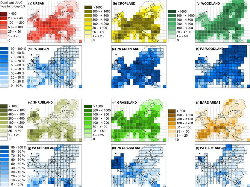
V. Reinhart et al.: The LANDMATE PFT map for Europe 2015 1737
LULC change representation among the FPS LUCAS RCM
ensemble is met. For the preparation of LANDMATE PFT,
we developed a CWP for the translation of LULC classes of
ESA-CCI into 16 PFTs according to the needs of regional cli-
mate modellers from all over Europe (Bontemps et al., 2013).
The focus in development of the LANDMATE PFT map Ver-
sion 1.0 is on the distinguished representation of biophysi-
cal properties in the RCMs, while the representation of bio-
chemical properties of different LC types will be addressed
in a future approach. A key issue to address in the map de-
velopment process is the accuracy of LULC representation
in the final product (Hartley et al., 2017). In order to assess
the quality of the product, we compared the LANDMATE
PFT map to a comprehensive ground truth database for large
parts of the European continent. The quality information de-
rived from the assessment supports the RCM community in
addressing and interpreting uncertainties caused by LULC
representation in RCMs. The general workflow and subse-
quently all utilized datasets are summarized in Sect. 2, while
the major steps of the CWP are listed in Sect. 3. Section 4
introduces in detail the accuracy assessment procedure, fol-
lowed directly by the results in Sect. 5. All CWTs and figures
corresponding to the CWP and the accuracy assessment can
be found in Appendices A and B.
2 Methods and data
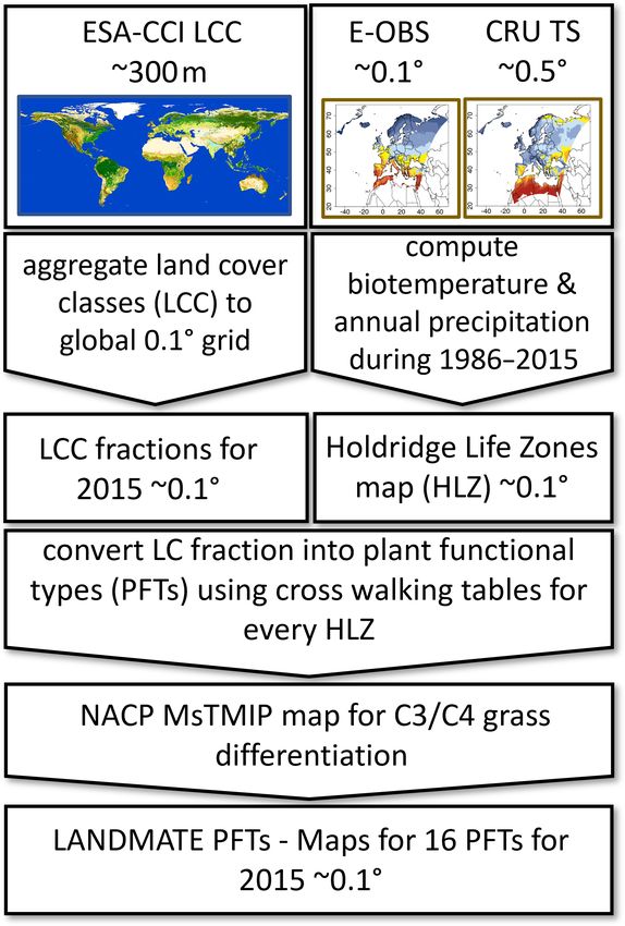
The LANDMATE PFT map (Reinhart et al., 2021b) is a com- Figure 1. The general workflow to generate LANDMATE PFT
bination of multiple datasets and concepts created using well- 2015 Version 1.0. This workflow is part of the workflow to gen-
established methods and, in addition, by considering the ex- erate the LUCAS LUC time series as introduced in the companion
pertise of regional climate modellers from all over Europe paper by Hoffmann et al. (2021).
within the FPS LUCAS.
tion from 1950 to 2020 are used to create the climate zone
2.1 General workflow
map of 0.1◦ horizontal resolution which is further imple-
The workflow to generate the LANDMATE PFT map is sum- mented in the CWTs to prepare the final LANDMATE PFT
marized in Fig. 1, which also includes the steps to generate maps. For regions that are not covered by E-OBS, the re-
the LUCAS LUC dataset further described in the companion spective data of the Climate Research Unit (CRU) dataset
paper by Hoffmann et al. (2021). First, a high-resolution land (Sect. 2.2.3) are used.
cover map (ESA-CCI LC, Sect. 2.2.1), which has a native A CWT (Sect. 3) is created for each of the 37 ESA-CCI
resolution of ∼ 300 m, is aggregated to the 0.1◦ target resolu- LC classes. Since the table has three dimensions (land cover
tion using SAGA GIS (Conrad et al., 2015). The target reso- class, HLZ and PFT), it was necessary to prepare the indi-
lution results from the FPS LUCAS ensemble resolution (i.e. vidual tables that include unique translations for each HLZ.
EURO-CORDEX domain EUR-11) that is used for LULCC For example, Table 1 shows the CWT for LC class 40 –
impact studies in FPS LUCAS Phase II. The LULC type in- Mosaic natural vegetation (tree, shrub, herbaceous cover)
formation from the original product is preserved in fractions (> 50 %)/cropland (< 50 %) – where the numbers of the
per 0.1◦ grid cell, which is advantageous to common ma- HLZs in the first column correspond to the HLZ numbers
jority resampling methods. The sum of PFT fractions in the in Fig. 2. For each HLZ in the first column, LC class 40 is
whole dataset remains the same at all target resolutions: only translated into fractions of the LANDMATE PFTs. For the
the distribution of fractions per grid cell changes depending example class that means an increasing tree fraction from the
on the target resolution. boreal to tropical HLZs and a change in tree species compo-
A climate dataset for Europe (E-OBS, Sect. 2.2.2) is uti- sition which makes the whole PFT fraction composition per
lized for the preparation of a climate zone map over Europe pixel regionally adjustable. Each pixel of the map that con-
(Holdridge life zones, Sect. 2.2.4). From the climate dataset, tains one specific ESA-CCI LC class is translated to contain
the ensemble means 2 m temperature and annual precipita- multiple PFT fractions representing the properties of multi-
https://doi.org/10.5194/essd-14-1735-2022 Earth Syst. Sci. Data, 14, 1735–1794, 2022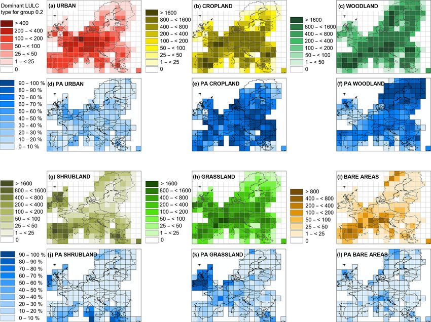
1738                                                               V. Reinhart et al.: The LANDMATE PFT map for Europe 2015

ple LC types, such as roughness length, albedo or leaf area           with random perturbations in order to produce an ensemble
index. These multiple properties can further be implemented           of realizations. For the creation of the HLZs that are used for
in an RCM. Depending on the ability of the RCM, multiple              the conversion of ESA-CCI LC classes to PFTs (Sect. 2.2.5),
fraction properties or an average of the properties are passed        the ensemble mean of the 2 m temperature (TG) and precipi-
on to the overlaying and underlaying layers, where the aver-          tation (RR) on a regular 0.1◦ grid from E-OBS Version 19.0e
age of all PFT fraction properties is still a more accurate rep-      is used. It covers most of Europe, some parts of the Middle
resentation of LC than the properties of only one LC class.           East and a narrow strip of northern Africa.
An example of the implementation of PFT fractions in an
RCM is given by Wilhelm et al. (2014), where the use of               2.2.3   CRU
PFTs within the RCM REMO is described.
   The translation process is based on Wilhelm et al. (2014),         The CRU TS 4.03 dataset is a global gridded high-resolution
where the translation of the Global Land Cover (GLC) 2006             climate dataset based on station observations produced and
into the 16 REMO-iMOVE PFTs is described. Since the                   maintained by the CRU of the University of East Anglia
nomenclatures of GLC 2006 and ESA-CCI LC are similar                  (Harris et al., 2014). The dataset provides global monthly
and based on the same classification system, some of the              means of climate parameters at 0.5◦ resolution from 1901
CWTs were initially adopted from Wilhelm et al. (2014). For           to 2019. In order to achieve the target resolution of 0.1◦ for
the more diverse ESA-CCI LC classes, new CWTs need to                 the global LANDMATE PFT maps, the CRU climate data
be created. The new CWTs follow the translation of Poulter            are downscaled using bilinear interpolation. Following Hoff-
et al. (2015) (ESA POULTER) but were carefully revised and            mann et al. (2016), distance-weighted interpolation was ap-
modified during the process. After application of the CWP,            plied to the atmospheric observation dataset CRU to extrap-
an additional map of potential C3 and C4 grass vegetation             olate the climate data to the coastlines of the ESA-CCI LC
(North American Carbon Program Multi-scale Synthesis and              maps in order to compensate for the different land–sea masks
Terrestrial Model Intercomparison Project – NACP MsTMIP,              of the products. The CRU climate dataset was used within
Sect. 2.2.6) is used to divide the grass PFT fractions. The           this application for regions where E-OBS is not available.
quality of the LANDMATE PFT dataset is finally assessed by            The bilinear interpolation of E-OBS caused minor issues on
comparison to a comprehensive ground truth database (LU-              coastlines and small islands all over the research area, where
CAS land use and land cover survey, Sect. 4).                         this interpolation method was not able to correctly account
                                                                      for the resolution differences of the 0.1◦ E-OBS and 0.018◦
2.2     Datasets and concepts                                         LANDMATE PFT land–sea masks, respectively. The issue
                                                                      caused by the large resolution difference is fixed with a pre-
2.2.1    ESA-CCI LC                                                   ceding extrapolation of the climate data along coastlines and
The ESA-CCI provides continuous global land cover maps                islands in the LANDMATE PFT map Version 1.1 that is cur-
(ESA-CCI LC) at ∼ 300 m horizontal grid resolution. The               rently being prepared. Since the interpolation issue only af-
ESA-CCI LC maps are available for download in annual                  fected a negligible number of LANDMATE PFT cells, the
time steps for the years 1992–2018 (ESA, 2017a). The clas-            validation measures are not affected by this issue in a notice-
sification of the LC maps follows the United Nations Land             able way.
Cover Classification System (UN-LCCS) protocol (Di Gre-
gorio, 2005) and consists of 22 level-1 classes and 14 ad-            2.2.4   Holdridge life zones
ditional level-2 classes, which include regional specifica-
tions. More information on ESA-CCI LC data processing can             The Holdridge life zone concept was initially developed in
be found at http://maps.elie.ucl.ac.be/CCI/viewer/download/           1967 (Holdridge, 1967) to define all divisions of the global
ESACCI-LC-Ph2-PUGv2_2.0.pdf (last access: 4 April 2022                biosphere, depending on the relation of biotemperature (aver-
). An overview of the satellite missions involved in the pro-         age of monthly temperature above 0◦ C; since plant activities
duction of ESA-CCI LC is given in Table 2. Besides sys-               are idle below freezing, all values below 0◦ C are adjusted
tematic global validation efforts (ESA, 2017a; Hua et al.,            to 0◦ C), mean annual precipitation and the ratio of potential
2018), a few regional approaches investigated the quality of          evapotranspiration to mean annual precipitation. By combin-
ESA-CCI LC over Europe (Vilar et al., 2019; Reinhart et al.,          ing threshold values of biotemperature and annual rainfall,
2021a).                                                               the 38 HLZs are created (Table 3). In the present analysis,
                                                                      the subtropical and warm temperate as well as polar and sub-
                                                                      polar HLZs are merged. Through the merging of the afore-
2.2.2    E-OBS climate data
                                                                      mentioned HLZs, 30 individual HLZs in total are available
The E-OBS dataset (Cornes et al., 2018) is a daily gridded            for the creation of the European HLZ map (Fig. 2).
observational dataset derived from station observations from             The dynamic character of the specific quantitative ranges
European countries covering the period from 1950 to 2020.             of the long-term means of the utilized climate parameters
The point observations are interpolated using a spline method         makes the HLZ classification more flexible than other avail-

Earth Syst. Sci. Data, 14, 1735–1794, 2022                                            https://doi.org/10.5194/essd-14-1735-2022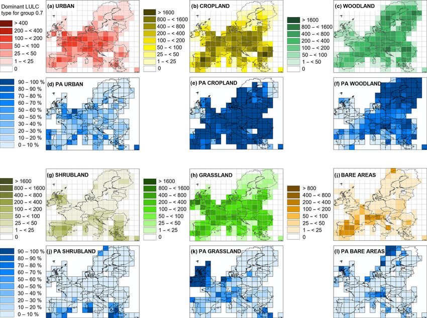
Table 1. Cross-walking table for ESA CCI LC class 40 – Mosaic natural vegetation (tree, shrub, herbaceous cover) (> 50 %)/cropland (< 50 %).
1 2 3 4 5 6 7 8 9 10 11 12 13 14 15 16
Tree Shrub Grass Special veg. Crops Non-veg.
Holdridge life Trop. broadl. Trop. broadl. Temp. broadl. Temp. broadl. Evergr. Decid. Evergr. Decid. C3 C4 Tundra Swamps Crops Irrig. Urban Bare
zone evergr. decid. evergr. decid. conif. conif. ground
1, 2 35 30 35
https://doi.org/10.5194/essd-14-1735-2022
3–5 30 35 35
6 25 40 35
7 60 40
8 10 50 40
9, 10 15 45 40
11 20 40 40
12 30 20 10 40
13 10 10 10 30 40
V. Reinhart et al.: The LANDMATE PFT map for Europe 2015
14, 15 20 20 10 10 40
16 25 20 15 40
17 25 25 10 40
18 30 30 40
19 60 40
20 35 25 40
21 20 15 15 10 40
22 25 10 15 10 40
23, 24 20 20 20 40
25 60 40
26 30 30 40
27 10 50 40
28 40 20 40
29 40 20 40
30 50 10 40
Earth Syst. Sci. Data, 14, 1735–1794, 2022
1739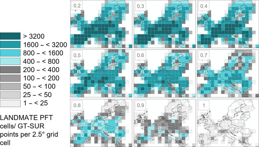
1740                                                                          V. Reinhart et al.: The LANDMATE PFT map for Europe 2015

Table 2. Satellite missions involved in the production of ESA-CCI LC according to ESA (2017a).

                           Time period                 Satellite product
                           Baseline production         MERIS FR/RR1 global SR2 composites
                           2003–2012
                           1992–1999                   Baseline 10-year global map; AVHRR3 global SR composites
                                                       for back-dating the baseline
                           1999–2013                   Baseline 10-year global map; SPOT-VGT4 global SR com-
                                                       posites for updating and back-dating the baseline; PROBA-V5
                                                       global SR composites at 300 m
                           2013–2015                   Baseline 10-year global map; PROBA-V global SR composites
                                                       at 1 km for the years 2014 and 2015 for updating the baseline;
                                                       PROBA-V time series at 300 m
                           Since 2016                  Sentinel-3 OLCI and SLSTR6 7 d composites
                         1 MEdium Resolution Imaging Spectrometer Full Resolution/Reduced Resolution (ESA, 2006). 2 Surface
                         reflectance. 3 Advanced Very-High-Resolution Radiometer (Hastings and Emery, 1992). 4 SPOT Vegetation
                         satellite programme (Maisongrande et al., 2004). 5 Project for On-Board Autonomy – Vegetation (Dierckx et al.,
                         2014). 6 Ocean and Land Colour Instrument (OLCI) and Sea and Land Surface Temperature Radiometer (SLSTR)
                         (Donlon et al., 2012).

Table 3. The Holdridge life zones following Holdridge (1967).

   Bio-                                                                          Precipitation (mm)
   temperature
   (◦ C)
                 < 125                 125 to < 250               250 to < 500               500 to < 1000              1000 to < 2000        > 2000
    24          Tropical desert       Tropical desert shrub      Tropical thorny wood-      Tropical very dry forest   Tropical dry forest   Tropical
                                                                  land                                                                        moist/wet/rain
                                                                                                                                              forest

able global ecosystem classifications and therefore makes the                       PFT maps become more detailed and can be customized to
HLZs most suitable for the application presented in this ar-                        individual regions without losing global consistency.
ticle. In addition, the requirement for input data is relatively
low.                                                                                2.2.5     Plant functional types
   In the past, the HLZ concept was not only found to be
useful for global applications, but was also successfully im-                       Figure 3 shows the LANDMATE PFTs that are based on the
plemented, especially for regional mapping approaches, due                          PFTs introduced by Wilhelm et al. (2014). The implementa-
to its ability to capture regional climate features with the                        tion of an irrigated cropland PFT (PFT 14) that is currently
support of bioclimatic variables (Daly et al., 2003; Tatli and                      being developed within the HICSS project LANDMATE will
Dalfes, 2016). Further, the HLZ concept was used for LULC                           be implemented in a later version of the dataset. In the initial
change predictions, such as land use impact assessments, re-                        version that is presented in this article, all cropland propor-
lated to current and future climate change scenarios (Chen                          tions are assigned to the cropland PFT (PFT 13).
et al., 2003; Skov and Svenning, 2004; Yue et al., 2006; Saad
et al., 2013; Szelepcsényi et al., 2018). With the implemen-
tation of climate data through the HLZ concept, the resulting

Earth Syst. Sci. Data, 14, 1735–1794, 2022                                                               https://doi.org/10.5194/essd-14-1735-2022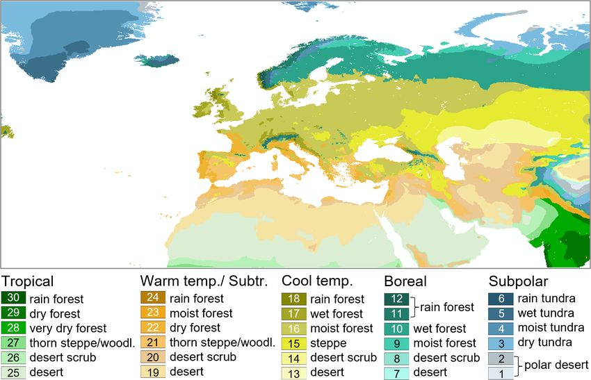
V. Reinhart et al.: The LANDMATE PFT map for Europe 2015                                                                           1741

Figure 2. Holdridge life zone map for the extent of LANDMATE PFTs.

Figure 3. LANDMATE PFT map for Europe for 2015 (a). Below a map section of the Alpine region shows an example of the resolution
difference between LANDMATE PFT 0.1 (b) and LANDMATE PFT 0.018 (c). LANDMATE PFT 0.018 is used in the present accuracy
assessment. For improved visualization, all maps show the majority PFT per grid cell. The irrigated cropland PFT (14) is not used in this
map. More information is given in Sect. 3.4.

https://doi.org/10.5194/essd-14-1735-2022                                              Earth Syst. Sci. Data, 14, 1735–1794, 2022
1742                                                              V. Reinhart et al.: The LANDMATE PFT map for Europe 2015

2.2.6    Potential C4 grass fraction NACP MsTMIP                     tries. Throughout the survey, the ground truth data were con-
                                                                     tinuously checked for quality and plausibility. For the accu-
The initial land cover map from the ESA-CCI LC does not              racy assessment of the LANDMATE PFT map, the ground
provide a distinction between C3 and C4 grassland. The fo-           truth points of the year 2015 are employed (Sect. 4). In order
cus of the present approach is the improvement of represen-          to avoid confusion between the FPS LUCAS and the LUCAS
tation of the biophysical properties of LC types. Since the          ground truth dataset, the latter will be further referred to as
distinction between C3 and C4 grasses is rather important            ground truth survey or GT-SUR.
for biochemical properties, such as the carbon cycle, the de-
cision was made to use a pre-existing, external product for
the spatial distinction between C3 and C4 grasses. The map           3     Cross-walking procedure – ESA-CCI LC classes to
from the NACP MsTMIP (Wei et al., 2014) is constructed                     PFTs
based on the synergetic land cover product (SYNMAP) by
Jung et al. (2006). SYNMAP is a combination of multiple              The CWP from ESA-CCI LC classes to PFTs presented in
high-resolution LULC products using a fuzzy agreement ap-            this article is based generally on (1) the translation intro-
proach. The NACP MsTMIP map uses the grassland frac-                 duced by Poulter et al. (2015) and (2) the translation by
tions from the SYNMAP product. The potential C4 grass                Wilhelm et al. (2014). Both translations are not just com-
distribution is generated by Wei et al. (2014) by employing          bined with each other, but are also modified using additional
the well-established method introduced by Still et al. (2003),       data. The following sections introduce the PFTs of LAND-
which is based on the growing season temperature and rain-           MATE PFT aggregated into general LULC types and give an
fall in combination with present climate conditions from the         overview of the decisions on modifications that are made dur-
global CRU-NCEP dataset. The potential C4 grass map is               ing the production process based on literature and additional
provided on a 0.5◦ horizontal grid for the period from 1801          data.
to 2010. For the preparation of LANDMATE PFT the NACP
MsTMIP map of 2010 is used. The LANDMATE PFT grass
fraction is split up into C4 and C3 grasses by multiplying           3.1    Trees and shrubs, tropical and temperate | PFTs
grassland by the potential C4 vegetation fraction and for C3                1–8
grass (1 – potential C4 vegetation fraction), respectively.          The LANDMATE PFTs are more diversified regarding tree
   The spatial distribution of C3 and C4 grasses is not evalu-       PFTs than the generic ESA POULTER PFTs. While the
ated in the present approach due to the lack of information in       generic ESA POULTER PFTs have four shrub PFTs, the
the reference dataset. Through the use of the state-of-the-art       LANDMATE dataset has only two, while the tree PFT count
NACP MsTMIP map, the highest possible quality of C3 and              was increased to six. The increase in tree PFT diversity is
C4 grass distribution given in the LANDMATE PFT map is               done in order to address the strong biogeophysical impacts
ensured.                                                             of forested areas on regional and local climate, such as de-
                                                                     creased albedo and increased roughness length (Bright et al.,
2.3     LUCAS – land use and land cover survey                       2015). The effects of forested areas on near-surface climate
                                                                     are distinctively different to the effects of shrub- or grass-
The harmonized LUCAS in situ land cover and use database             covered areas and are also highly dependent on tree species
for field surveys from 2006 to 2018 (d’Andrimont et al.,             composition and latitudinal range (Bonan, 2008; Richardson
2020) is the most consistent ground truth database for the           et al., 2013). Another reason for the six tree PFTs is the in-
European continent. The survey was carried out at 3-yearly           tended use of the PFT maps in RCMs. In the land surface
intervals between 2006 and 2018. The systematic sampling             models (LSMs) of current-generation RCMs, a distinction is
design of the survey consists of a theoretical, regular grid         rather made between different tree or tree community types
over the European continent with ∼ 2 km grid size. The ref-          than between different shrub types. Therefore, and with re-
erence point locations are the corner points of the theoretical      gard to the implementation process that needs to be done for
grid. Not all locations within the survey were easily accessi-       each RCM individually, an increase in the number of tree
ble. Therefore, the survey is supported by in situ photo inter-      PFTs and a decrease in the number of shrub PFTs are consid-
pretation, in-office photo interpretation and satellite data in      ered to be convenient. Accordingly, the tree and shrub pro-
the latest time steps 2015 and 2018 (Table 4). However, the          portions were distributed following both the needleleaf and
main proportion of the reference points was recorded through         broadleaf definitions of the ESA-CCI LC classes as well as
location visits at all time steps, which makes this land survey      the HLZ map, where the HLZ map was decisive for an as-
the most reliable and consistent ground truth database for Eu-       signment of forest proportions to the temperate or tropical
rope.                                                                tree PFT, respectively. Following a comparison to different
   The extent of the LUCAS survey was increased over time.           forest datasets over Europe (not shown), the tree proportions
The 2006 survey covered 11 countries, while the 2018 map             in the translation of the mixed land cover classes, e.g. class
covers large parts of the European continent, with 28 coun-          61 – Tree cover, broadleaved, deciduous, closed (> 40 %),

Earth Syst. Sci. Data, 14, 1735–1794, 2022                                           https://doi.org/10.5194/essd-14-1735-2022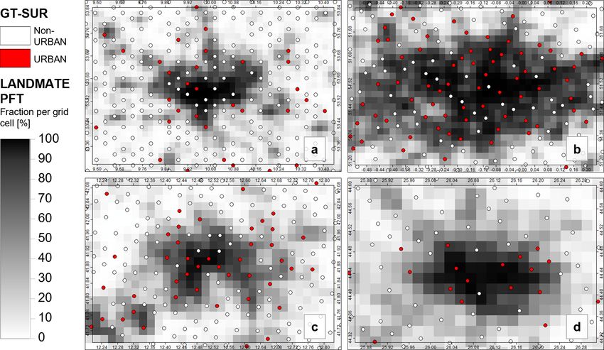
V. Reinhart et al.: The LANDMATE PFT map for Europe 2015                                                                                       1743

Table 4. Number and recording method of reference points in the LUCAS land cover and use database per time step.

                             Year       Reference points            In situ      In situ PI1       In-office PI2         GT3 (%)
                             2006             168 401             155 238           13 163                                   92.18
                             2009             234 623             175 029           59 594                                    74.6
                             2012             270 272             243 603           26 669                                   90.13
                             2015             340 143             242 823           25 254             71 970                71.39
                             2018             337 854             215 120           22 894             99 803                63.67
                           1 Photo interpretation close to the reference location. 2 Photo interpretation with supporting data, such as
                           satellite images. 3 Ground truth.

are increased to be in line with the indicated overall forest                       classes and mixed cropland classes into the cropland PFTs
amount over Europe.                                                                 were investigated by Li et al. (2018), where the comparison
                                                                                    of LULC change in the ESA POULTER PFT maps against
3.2   Grassland | PFTs 9 and 10                                                     other LULC products showed inconsistencies between global
                                                                                    trends and geographical patterns between the products. How-
The generic ESA POULTER PFTs include a natural grass-                               ever, Li et al. (2018) provide a modified CWT that was ad-
land and a managed grassland PFT to include grassland and                           justed with regard to an improved knowledge base on how to
cropland, respectively. The LANDMATE PFTs include two                               translate LULC classes into PFTs for climate models. Partic-
grassland PFTs, distinguishing between C3 and C4 grass. The                         ular focus is laid on mosaic classes and the sparsely vegetated
contrasting photosynthetic pathways and therefore contrast-                         classes, of which numerous appear in ESA-CCI LC. There-
ing synthetic response to CO2 and temperature determine                             fore, the CWP from Li et al. (2018) for cropland is adopted
specific ecosystem functions for both PFTs, respectively. The                       in the present CWP.
main differences are found in global terrestrial productiv-                            The irrigated cropland PFT (PFT 14, Fig. 3) is currently
ity and water cycling (Lattanzi, 2010; Pau et al., 2013). The                       empty in the LANDMATE PFT map Version 1.0. This de-
translation from the LULC classes that contain grassland pro-                       cision is made following intense research on available irri-
portions into C3 or C4 grass PFTs, respectively, is supported                       gation information. The ESA-CCI LC map that is used as
by a map of potential C4 vegetation by Wei et al. (2014),                           initial input contains an “irrigated cropland” class, but this
where the potential global distribution of C4 is estimated us-                      information was not used in the process. The investigation
ing bioclimatic parameters (Sect. 2.2.6).                                           on irrigated areas included the comparison of ESA-CCI LC
                                                                                    to other products that are available, such as the irrigation map
3.3   Tundra and swamps | PFTs 11 and 12                                            from the FAO (Siebert et al., 2005). Although the ESA-CCI
                                                                                    LC quality assessment shows very good agreement of the
The specific vegetation PFTs tundra and swamps are treated                          ESA-CCI LC irrigated cropland with the validation database
individually in LANDMATE PFT. Tundra is mostly used for                             (ESA, 2017a), the comparison showed considerable differ-
the polar and subpolar HLZs, where the climatic conditions                          ences between the products. The success of detection of irri-
require a clear distinction of the land surface properties from                     gated areas is highly dependent on the correct detection of the
the boreal and temperate regions regarding exchange and                             crop types to infer the water needs of the respective crops, on
feedback processes with the atmosphere (Thompson et al.,                            atmospheric and environmental conditions and on the avail-
2004). Chapin et al. (2000) further suggest a differentiation                       ability of multi-temporal, high-resolution imagery (Bégué
of vegetation composition within these northern vegetation                          et al., 2018; Karthikeyan et al., 2020). Further, most remote
communities, which can also be realized using the intro-                            sensing applications depend highly on ground truth data and
duced CWP. The swamp PFT is mostly used for translating                             local knowledge. Applications using different satellite im-
the ESA-CCI LC mosaic tree/shrub/herbaceous classes and                             agery to detect agricultural management practices, such as
also partly for the flooded tree cover classes in most of the                       irrigation, are only successfully tested and applied in local
HLZs. Swamps occur mainly in the boreal and polar regions                           spatial units (Rufin et al., 2019; Ottosen et al., 2019). There-
in the European domain.                                                             fore, the irrigated cropland PFT remains unoccupied for now.
                                                                                    Nevertheless, PFT 14 is defined within LANDMATE PFT
3.4   Cropland | PFTs 13 and 14                                                     Version 1.0 for the purpose of adding irrigated LULC frac-
                                                                                    tions in the future. For the long-term LUCAS LUC dataset
Currently, two cropland PFTs are defined in the LAND-                               (Hoffmann et al., 2021), which is extended backward and for-
MATE PFT map. The cropland PFT (PFT 13, Fig. 3) in-                                 ward based on the LANDMATE PFT map for Europe 2015,
cludes all managed, agricultural land surface proportions.                          irrigated cropland areas are already implemented following
The uncertainties of the translation of the ESA-CCI cropland

https://doi.org/10.5194/essd-14-1735-2022                                                                 Earth Syst. Sci. Data, 14, 1735–1794, 2022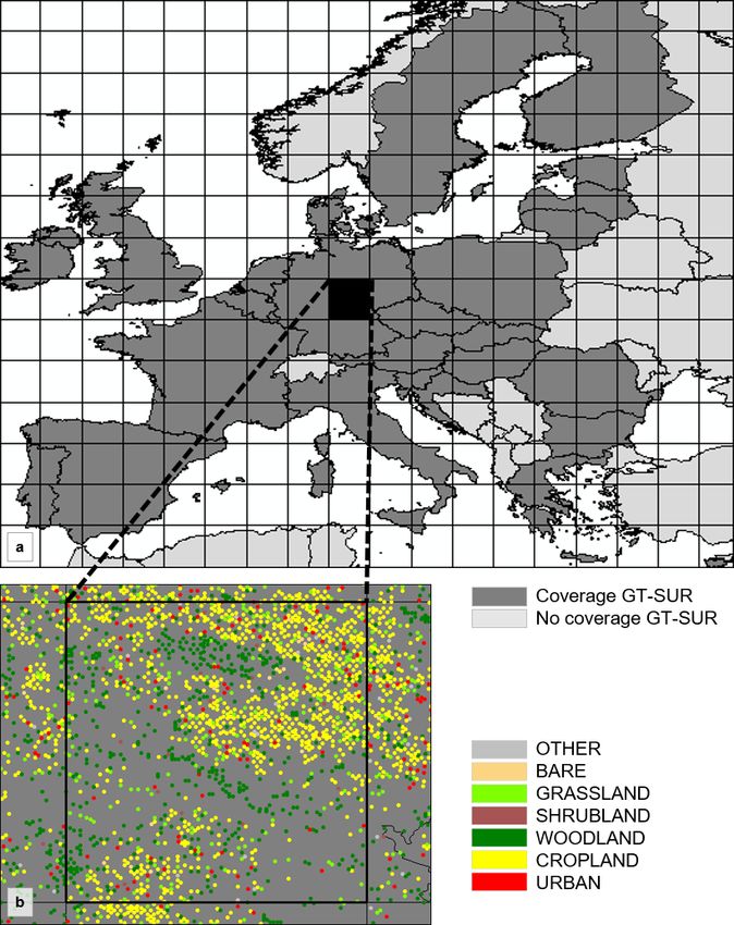
1744                                                                V. Reinhart et al.: The LANDMATE PFT map for Europe 2015

the irrigated area definition of the Land Use Harmonization
(LUH2) dataset (Hurtt et al., 2011).

3.5    Non-vegetated | PFTs 15 and 16
The non-vegetated PFTs in the LANDMATE PFT dataset are
urban and bare. The urban grid cells from ESA-CCI LC are
directly translated into urban fractions for all HLZs in the
CWP. The same applies for all bare ground proportions that
are translated fully into the bare PFT. In addition, the ESA-
CCI LC mixed classes are split up, and the bare ground pro-
portions within the mixed classes are added to the bare PFT.
The explicit treatment of urban areas and especially differen-
tiation from bare ground provides the possibility of resolving
urban surface characteristics in RCMs. The treatment of ur-
ban areas as a slab surface or as an equal to rock surface
as done in several RCM approaches cannot account for the
complex biogeophysical processes associated with an urban
agglomeration (Daniel et al., 2019; Belda et al., 2018). Due
to the distinction of the two surface types, the LANDMATE
PFT map can be used for impact studies with an urban focus.

3.6    Water, permanent snow and ice
The LANDMATE PFTs do not include individual PFT defi-
nitions for water and snow/ice, respectively. Regarding the
water representation, most currently used RCMs utilize a               Figure 4. Coverage of the reference GT-SUR over the European
land–sea mask to account for oceans and inland water ar-               continent (a). As an example for the whole research area (b) shows
eas. Therefore, an explicit definition of water as an individ-         the GT-SUR point coverage (and LULC group representation) of
ual PFT has not been implemented. Consequently, all water              one grid cell of the auxiliary 2.5◦ grid.
fractions such as marine water, lakes and rivers are set to no
data. In the present translation, the snow/ice grid cells from
ESA-CCI land cover are translated into a bare PFT following            and nomenclature, given that ground truth reference data are
Wilhelm et al. (2014).                                                 mostly collected as point data and independently of the as-
                                                                       sessed map product (Foody, 2002; Wulder et al., 2006; Olof-
                                                                       sson et al., 2014). In order to produce reliable quality infor-
4     Quality assessment of the LANDMATE PFT map
                                                                       mation for LANDMATE PFT, the present assessment fol-
The LANDMATE PFT map is based on the ESA-CCI LC                        lows closely the well-established good-practice recommen-
map which was quality checked and compared to similar                  dations. Nevertheless, adjustments are done to account for
LULC products on a global (ESA, 2017b; Yang et al., 2017;              the fractional structure of LANDMATE PFT. Section 4.2
Hua et al., 2018; Li et al., 2018) and regional level (Rein-           provides additional information on the requirements of a
hart et al., 2021a; Vilar et al., 2019). However, the translation      good-practice accuracy assessment, the key components and
from LULC classes into PFTs necessarily results in a change            the selected sampling design and metrics.
in the map. The final product, the LANDMATE PFT map,
is intended to be used in RCMs, which means the quality of             4.1   Research area
the final product must be assessed in addition to the avail-
able quality assessments of the initial ESA-CCI LC map. In             The coverage of GT-SUR in the year 2015 includes 28 coun-
order to overcome the resolution difference, which is non-             tries which are highlighted in dark grey in Fig. 4.
negligible between LANDMATE PFT and the reference data                    The total number of GT-SUR points for 2015 is 340 143.
GT-SUR, the LANDMATE PFT map is prepared at 0.018◦                     Out of these points, 338 619 points (∼ 99.55 %) are cov-
horizontal resolution, which corresponds closely to the 2 km           ered with valid LANDMATE PFT grid cells of the assessed
theoretical grid of GT-SUR.                                            LULC types and can be used in the analysis. Countries
   The design of such a quality assessment of a large-scale            located within the contiguous area but missing in the as-
map product is not trivial, especially since the map product           sessment are Switzerland, Norway, the Russian Kaliningrad
itself and the reference data are often different in structure         Oblast, Bosnia and Herzegovina, Montenegro, Albania, Ser-

Earth Syst. Sci. Data, 14, 1735–1794, 2022                                              https://doi.org/10.5194/essd-14-1735-2022
V. Reinhart et al.: The LANDMATE PFT map for Europe 2015 1745
bia, Kosovo, North Macedonia, and Belarus. Figure 4 also with every unit of LANDMATE PFT containing more than
shows the 2.5◦ grid that was used for the analysis of the ac- one LULC type potentially. Therefore, the subsets are se-
curacy assessment results (Sect. 5). Due to the fine scale and lected through application of a filter to capture the map accu-
the high number of points over the whole research area, the racy in a way that accounts for the fractional structure within
visualization of the spatial analyses on a continental scale is the grid cells in the LANDMATE PFT map (see Sect. 4.2.1).
challenging. Therefore, the research area is overlayed with a The response design deals with the spatial support regions
2.5◦ grid (as shown in Fig. 4). While the results are presented (SSRs) and the labelling protocol or classification harmo-
in these 2.5◦ grid units, the results are calculated for each nization. The SSR is a buffer region around a sampling unit
point within one unit and then aggregated. For example, in that is selected to account for small-scale landscape hetero-
a 2.5◦ grid unit containing 1000 pairs of LANDMATE PFT geneity that is likely not captured by larger-scale map prod-
cells and GT-SUR points, 50 % overall accuracy is achieved ucts. In the present case, the sampling design is selected in a
when 500 pairs agree on the LC type. The overall and class- way that the grid cells of LANDMATE PFT serve as SSRs
wise accuracy results for all points within each 2.5◦ grid cell for each GT-SUR point. A fraction is not located precisely
are aggregated in order to identify large-scale spatial quality at one location within the respective grid cell but is evenly
differences for the analysed LULC types. In order to give in- distributed over the whole grid cell. Assuming the uniformly
formation on the relevance of the accuracy metrics, the num- distributed fraction can occur in small patches or in one large
ber of LANDMATE PFT–GT-SUR pairs for each LULC type patch within the grid cell, the whole grid cell is defined as
per grid cell are displayed alongside the accuracy figures in an SSR for the respective LULC type. The labelling proto-
Sect. 5. col needs to be determined to deal with the different legends
of the reference and the assessed map. The harmonization of
4.2 Accuracy assessment – background and design
legends is selected with regard to the objective of the respec-
tive assessment, as in this case, to provide information about
The key components of the accuracy assessment of a large- the quality of representation of the most dominant LULC
scale land cover product are objective, sampling design, re- types in LANDMATE PFT. The labelling protocol used in
sponse design and the final analyses and estimation (Wulder the present assessment is summarized in Table 5.
et al., 2006). All of the key components have great impact The analyses and estimation used are error matrices that
on the quality of the assessment and, further, on the final give an overview of the overall and LULC type-wise accu-
metrics, especially in the present assessment, where refer- racy of the LANDMATE PFT map. For both resolutions of
ence and assessed dataset differ widely in structure. LAND- LANDMATE PFT, the error matrices and the resulting ac-
MATE PFT is a gridded dataset with fractional LULC classes curacy measures overall accuracy (OA), producer’s accuracy
but no information on the subgrid location within the grid (PA) and user’s accuracy (UA) are calculated, where PA and
cell. Other than that, the points of GT-SUR have fixed lo- OA are calculated group-wise. The error matrix is a cross-
cations expressed through exact coordinates but no (exact) tabulation between map and reference of the size q×q, where
information on the spatial extent of this class. Another chal- q stands for the number of land cover classes or groups. The
lenge is the fractional structure of LANDMATE PFT itself, map classes are placed in the rows and the reference classes
where one unit (grid cell) possibly contains multiple frac- in the columns so that the diagonal of the matrix gives the
tions. Therefore, the design of the accuracy assessment needs sum of the correctly classified map units. The off-diagonal
to be customized to the objective, which is to determine the cell values represent the disagreement between the map and
overall quality of the LANDMATE PFT map for Europe the reference. The overall accuracy is calculated according to
2015 as well as the quality of individual LULC type repre- Eq. (1):
sentation within the map in order to derive recommendations Pq
for the use of LANDMATE PFTs in RCMs. nii
OAi = i=1 × 100. (1)
When it comes to the sampling design, sampling size, spa- n
tial distribution of the respective sample and the representa-
The sum of the agreeing diagonal elements nii of all
tion of each LULC type or class within the sample are cru-
LULC types is divided by the number of all observations n.
cial for producing reliable quality information about a LULC
The PA represents the accuracy from the view of the map pro-
product (Stehman, 2009). The collection of ground truth data
ducer. The PA stands for the probability that a LULC feature
is a rather expensive procedure regarding time and money,
in the reference is classified as the respective feature by the
which needs to be considered during the process. However,
map. The PA is calculated using Eq. (2), where the number
in the present assessment we are able to rely on an exist-
of correctly classified units per LULC type nii is divided by
ing ground truth database containing over 340 000 records,
the total number of LULC type occurrences of the reference
which eliminates the possible issue of a too small reference
n+i :
database. It is also known that all assessed LULC types are
represented in a sufficiently high number (Table 6). Never- nii
theless, the present assessment is a special case situation, PAi = × 100. (2)
n+i
https://doi.org/10.5194/essd-14-1735-2022 Earth Syst. Sci. Data, 14, 1735–1794, 20221746 V. Reinhart et al.: The LANDMATE PFT map for Europe 2015
While the PA gives the proportion of features in the ref- while the GT-SUR points have fixed locations on the map.
erence that are actually represented as those in the produced With the applied grouping of the cells dependent on the min-
map, the UA is the accuracy from the perspective of the map imum coverage of the dominant LULC type, the influence
user. It is the probability of a feature classified as such in of grid cell heterogeneity on accuracy metrics is investigated
the map being actually present in the reference. The UA is within the assessment.
calculated using Eq. (3), where the number of correctly clas- Besides the total number of LANDMATE PFT cells in
sified
Pppixels nii per LULC type is divided by the row sum the analysis, diversity among the represented LULC types
ni+ i=1 nj i : is important. The right column of Table 6 shows the number
nii of LANDMATE PFT cells where the respective LULC type
UAi = × 100. (3) (left column) is dominant. The table is not grouped by min-
ni+
imum coverage but by LULC type and shows that each as-
sessed LULC type is represented in a sufficiently high num-
4.2.1 Dataset harmonization and filter
ber when only the cells with dominant coverage (regardless
The quality assessment is done by assigning the PFT type of the total proportion) are considered for each LULC type.
with the maximum fraction per grid cell to the GT-SUR
points located within the respective grid cell. The classifi-
cations of both datasets are harmonized as shown in Table 5, 5 Results
where the focus is laid on the main LULC types in order to
make the comparison as detailed as possible but also to be In order to show the impact of the grid cell heterogeneity of
able to produce reliable and robust results for the RCM com- LANDMATE PFT, the agreement of LANDMATE PFT with
munity. the reference GT-SUR is investigated for each threshold for
The LULC types URBAN, CROPLAND, WOODLAND, minimum coverage (0.1–1) of the dominant LULC type. For
SHRUBLAND, GRASSLAND and BARE AREAS are har- visualization of the spatial analysis, the point count and per-
monized without applying modifications to the classifica- centage agreement with the reference dataset are aggregated
tions. The LANDMATE PFTs can easily be grouped or di- per 2.5◦ cell of the auxiliary grid, which was established as
rectly adopted, while the GT-SUR level-1 classification (let- most useful for visualization of the results. Nevertheless, the
ters A–H) is completely adopted into the harmonized groups. comparison of LANDMATE PFT to GT-SUR is done at cell
In general, RCMs implement a dedicated land–sea mask level for the whole research area. All resulting confusion ma-
to determine aquatic areas for both inland and marine wa- trices for the assessed LC types at cell level are available in
ter. Therefore, the categories Water and Marine areas are Appendix B.
not further analysed. Since the LULC types Tundra and In order to be able to capture the spatial distribution of
Swamps (LANDMATE PFT) and Wetlands (GT-SUR) can- the quality of the LULC type representation within LAND-
not be harmonized with sufficient agreement with the GT- MATE PFT, the assessed cells must be distributed well over
SUR LULC type definitions, the LULC types are also not the research area and contain a sufficiently large cell count of
further analysed in the assessment. Thus, the LULC types each LULC type. Figure 5 shows the distribution and count
Water and Marine areas and Wetlands (GT-SUR) and Tundra of cells grouped by threshold for minimum coverage. The
and Swamps (LANDMATE PFT) are merged into the LULC maps show that the groups with a threshold lower than 0.7
type OTHER. Although the group cannot be evaluated re- are distributed very well over the research area. Each region
garding the quality of the LANDMATE PFT map, the group is covered with a sufficient number of LANDMATE PFT grid
needs to be involved in the assessment to keep the numbers cells that can be compared to the respective GT-SUR points.
in the assessment correct and reliable for all other groups. The 0.8 group shows a quite patchy pattern and a strongly
However, as is shown in Table 6, only a minor number of decreasing sample number in northern Europe. For the 0.9
points/cells is affected. group, the patchy pattern and low number of cells per 2.5◦
Both datasets are provided in a regular Gaussian grid grid cell spread over the whole research area. While the 0.9
(WGS84 EPSG:4326) so that no reprojection of the datasets group could still be used for evaluation of LANDMATE PFT
needs to be done for the comparison. for limited regions in Europe, the group only containing cells
The LANDMATE PFT dataset includes multiple LULC with 100 % coverage of one LULC type (map 1) is clearly not
fractions per grid cell. Accordingly, the area proportion of evaluable due to the overall small cell count (< 1500). Fig-
the dominant LULC type varies widely and thus the likeli- ure 6a gives an overview of the cell count per group for each
hood that the GT-SUR point sample falls within this area. individual LULC type.
The grid cells are grouped by minimum coverage of the dom- For CROPLAND, WOODLAND and GRASSLAND, the
inant LULC type from 0.1 to 1, where 0.1 means a minimum threshold for minimum coverage of the respective domi-
coverage of 10 % and 1 means full coverage of the domi- nant LULC type has a strong influence on the total cell
nant LULC type. The coexisting fractions are not located in count within each group, while for URBAN and BARE AR-
particular parts within a grid cell but are equally distributed, EAS, the cell count remains similar up to the 0.6 group. For
Earth Syst. Sci. Data, 14, 1735–1794, 2022 https://doi.org/10.5194/essd-14-1735-2022V. Reinhart et al.: The LANDMATE PFT map for Europe 2015 1747
Table 5. Classification harmonization between the LANDMATE PFT map and GT-SUR.
GT-SUR GT-SUR LANDMATE PFT LANDMATE PFT Harmonization Harmonization
LC group group name number name group number name
A Artificial land 15 Urban 1 URBAN
B Cropland 13 Non-irrigated crops 2 CROPLAND
14 Irrigated crops
C Woodland 1 Tropical broadleaf evergreen trees 3 WOODLAND
2 Tropical deciduous trees
3 Temperate broadleaf evergreen trees
4 Temperate deciduous trees
5 Evergreen coniferous trees
6 Evergreen deciduous trees
D Shrubland 7 Coniferous shrubs 4 SHRUBLAND
8 Deciduous shrubs
E Grassland 9 C3 grass 5 GRASSLAND
10 C4 grass
F Bare land 16 Bare 6 BARE AREAS
G Water 11 Tundra 7 OTHER
H Wetlands 12 Swamps
Other Marine areas
Table 6. General information on data in the comparison.
LULC type1 GT-SUR2 LANDMATE PFT LANDMATE PFT
0.018◦3 0.018◦ dominant4
URBAN 14 393 65 000 7577
CROPLAND 83 295 248 301 136 970
WOODLAND 124 374 277 290 124 437
SHRUBLAND 27 298 302 035 19 790
GRASSLAND 66 541 333 948 44 244
BARE AREAS 10 395 31 756 4148
OTHER 12 340 28 823 1470
Sums 338 636 338 636
1 LULC type analysed in the quality assessment. 2 Number of GT-SUR points per LULC type.
3 Total number of grid cells in LANDMATE PFT that have a share > 0 % of the respective LULC
type. 4 Number of cells where the LULC type is dominant in LANDMATE PFT 0.018◦ .
SHRUBLAND, the cell count decreases strongly from the Figure 6c shows the PA for all LULC types dependent on
0.4 group upwards. The curve characteristics suggest that the threshold for minimum coverage of the dominant LULC
the LULC types CROPLAND, WOODLAND, and GRASS- type, including the overall accuracy for all LULC types to-
LAND have a higher proportion of cells with a relatively low gether (dark grey line). While the overall accuracy is rela-
dominant coverage, but since they are the three most popu- tively independent of the threshold for minimum coverage,
lated LULC types overall (see Table 6), the proportions are some LULC types are affected. For WOODLAND, PA de-
comparable to the other three groups. creases rapidly for the 0.8 group. Considering that the cell
Figure 6b shows the highest UA for WOODLAND and the count for this group does decrease noticeably from 0.7 to
lowest for SHRUBLAND, while all the other LULC types 0.8 (Fig. 6a), the low PA is likely a result of this low cell
range in between. The threshold for minimum coverage of count. The PAs for GRASSLAND and SHRUBLAND re-
the individual LULC types has slightly more influence on main almost constant but at a lower level compared to the
the UA than on the PA of LANDMATE PFT, where the UA other groups.
increases towards the groups with higher cell homogeneity.
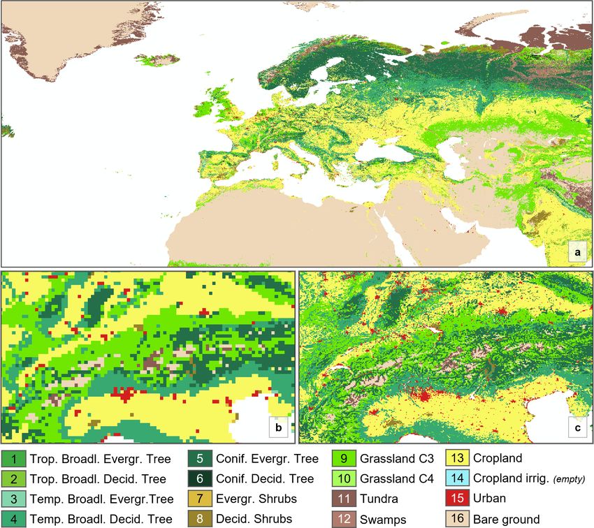
https://doi.org/10.5194/essd-14-1735-2022 Earth Syst. Sci. Data, 14, 1735–1794, 20221748 V. Reinhart et al.: The LANDMATE PFT map for Europe 2015 Figure 5. The distribution of the LANDMATE PFT cells grouped by threshold for minimum coverage of the respective dominant LULC type over the research area in Europe. The same number of LANDMATE PFT cells falls into the groups with minimum coverages of 0.1 and 0.2. Therefore, the 0.1 group is not shown in the figure. The spatial analysis for the six assessed LULC types for homogeneous sealed area. The LANDMATE PFT map rep- the 0.7 group is shown in Fig. 7. In order to give an overview resents this heterogeneous structure through the varying frac- of the spatial agreement patterns for the range of evaluable tions of non-urban PFTs within the grid cell. However, in or- groups, the respective figures for the 0.2 and 0.5 groups are der to make the impact of a larger city visible in an RCM included in Appendix B (Figs. B1 and B2). simulation, it is beneficial for LANDMATE PFT to repre- The urban representation in LANDMATE PFT for the 0.7 sent a larger city with a dense core structure. Further, the group is shown in Fig. 7a and d. Figure 6c shows that the PA URBAN fractions in LANDMATE PFT are directly adopted for all groups is overall low and not majorly influenced by from the ESA-CCI LC dataset, which was thoroughly val- the threshold for minimum coverage. With increasing cover- idated. Therefore, despite the low agreement with GT-SUR age of the dominant LULC type URBAN, the PA increases in the present assessment, the URBAN PFT of LANDMATE slightly but is still lower than 40 % for groups that include PFT 2015 is considered to be of sufficiently good quality and enough points to be considered representative of the research suitable for representing urban land cover in high-resolution area. (∼ 3 km) RCM simulations. Due to the aforementioned com- A visualization of the map agreement between LAND- parability issues, the UA of the LULC type URBAN is not MATE PFT and GT-SUR reveals the issue that leads to the further discussed in this assessment. overall low PA. Figure 8 shows four large URBAN agglomer- The CROPLAND representation in LANDMATE PFT ations in different areas of Europe, where the red points rep- shows, together with WOODLAND, the highest PA for the resent GT-SUR urban points and the white points represent research area. As shown in Fig. 6c, the PA for all 10 groups is GT-SUR points representing non-urban LULC types. The > 80 %, which is to be considered very good agreement with grey-scaled squares represent the LANDMATE PFT UR- the reference. BAN fractions from zero (no coverage, white) to one (full Figure 7b shows the distribution of CROPLAND points in coverage, black) within one grid cell. GT-SUR over the research area. CROPLAND points are the The LANDMATE PFT grid cells with a large urban frac- second-most frequent LULC type in GT-SUR and are mainly tion represent the respective city core of the selected example distributed over central and southern Europe. Although the cities, while the GT-SUR points that are located within the northern European grid cells show a lower count of CROP- city core are mostly not classified as URBAN. However, the LAND points, Fig. 7e shows that the PA is still very high GT-SUR points do not fail to represent the structure of urban in these areas. The PA increases with increasing cell homo- areas because these areas are characterized through a hetero- geneity (Figs. B1e and B2e). Regarding the UA for CROP- geneous pattern of sealed surfaces, recreational areas (e.g. LAND, LANDMATE PFT shows a strong overestimation, parks) and different building types and density, not through a where ∼ 36 % of the LANDMATE PFT CROPLAND cells Earth Syst. Sci. Data, 14, 1735–1794, 2022 https://doi.org/10.5194/essd-14-1735-2022
V. Reinhart et al.: The LANDMATE PFT map for Europe 2015                                                                   1749

                                                                   other LULC types (> 70 % for the 0.2 group and increasing
                                                                   towards the more homogeneous groups), which emphasizes
                                                                   the very good quality of WOODLAND representation in
                                                                   LANDMATE PFT. The most confusion is found with LULC
                                                                   type GRASSLAND and the OTHER LULC types (not inves-
                                                                   tigated in this assessment). Altogether, the UA of ∼ 85 % for
                                                                   group 0.7 is interpreted as a very good representation of the
                                                                   LULC type WOODLAND within LANDMATE PFT 2015.
                                                                      The coverage of cells with the dominant LULC type
                                                                   GRASSLAND is well distributed except for the northern
                                                                   European regions (Fig. 7h). The PA for LANDMATE PFT
                                                                   GRASSLAND according to Fig. 7k is very high in the United
                                                                   Kingdom and in some regions of central Europe. For the re-
                                                                   maining regions of the research area, the PA for GRASS-
                                                                   LAND is considerably low. This PA pattern remains simi-
                                                                   lar throughout the range of evaluable groups (Figs. B1k and
                                                                   B2k), with an average of 31 %–37 %.
                                                                      The main reason for this low accuracy of LANDMATE
                                                                   PFT regarding GRASSLAND can be found by looking at
                                                                   the results of the LULC types CROPLAND and WOOD-
                                                                   LAND. The UAs of CROPLAND and WOODLAND reveal
                                                                   that ∼ 36 % of the LANDMATE PFT CROPLAND cells ac-
                                                                   tually represent GRASSLAND in the reference, which adds
                                                                   up to over almost 55 % of the total GT-SUR GRASSLAND
                                                                   points. Another reason is found in the dataset structure of
                                                                   LANDMATE PFT. A considerable amount of GRASSLAND
Figure 6. Cell count (a), user’s accuracy (b) and producer’s ac-   is not part of the assessment because GRASSLAND does not
curacy (c) per LULC type of the LANDMATE PFT as a function         make up the dominant but rather the second-most dominant
of the threshold for minimum coverage of the respective dominant   PFT in ∼ 45 % of all LANDMATE PFT grid cells. There-
LULC type.                                                         fore, the seemingly weak GRASSLAND representation in
                                                                   LANDMATE PFT rather shows a weakness of the present
                                                                   assessment that is caused by the different dataset structures.
in the 0.7 group are actually another LULC type in the refer-         The PA for SHRUBLAND and BARE AREAS is the low-
ence, where 36 % are GRASSLAND and 13 % are WOOD-                  est of all assessed LULC types, with < 20 % for all groups
LAND. The UA for CROPLAND increases rapidly towards                of both LULC types, respectively (Fig. 6c). The low over-
the more homogeneous groups. However, the confusion with           all cell count of both LULC types might be one reason
WOODLAND and GRASSLAND is non-negligible and will                  for the low PA. However, looking at the distribution of the
be discussed in Sect. 7.                                           SHRUBLAND and BARE AREA points in Fig. 7g and i,
   For the representation of WOODLAND, the PA shows the            LANDMATE PFT is not able to capture the LULC types
second-highest values, with > 70 % for all groups with a rea-      even in grid cells with a relatively high cell count. The GT-
sonably high cell count (groups 0.1–0.7, Fig. 6c). Similar to      SUR includes ∼ 27 000 SHRUBLAND points, while LAND-
CROPLAND, the cell heterogeneity does not have a large             MATE PFT includes only ∼ 19 000 cells where SHRUB-
impact on PA. The highest PA is reached over the north-            LAND is the dominant LULC type. Therefore, one reason
ern European regions (Fig. 7f). Deficits are visible over the      for the poor SHRUBLAND representation lies within the
southern United Kingdom, parts of the Iberian Peninsula and        base map (ESA-CCI LC) used for the creation of LAND-
the coastline along Belgium and the Netherlands. Further, a        MATE PFT, where the known low count of SHRUBLAND
low PA is found for cells that have an overall small cell count    proportions was inherited by LANDMATE PFT. It must be
in the Mediterranean (Fig. 7c).                                    noted that a large proportion of SHRUBLAND in ESA-CCI
   The differences between northern and southern regions           LC is part of the mixed LC classes, such as Shrubland/Crop-
tend to increase towards the more homogeneous groups (see          land or Shrubland/Forest. The known deficit was partly com-
Figs. B1f and B2f for comparison). Agreement over the              pensated by the translation into the PFTs, where SHRUB-
northern regions increases, while agreement over the Iberian       LAND proportions were added to the total as proportions
Peninsula decreases together with a rapid decrease in the          of the mixed ESA-CCI LC classes. Further, SHRUBLAND
WOODLAND cell count within the corresponding grid cells.           makes up the second-most dominant PFT in ∼ 20 % of the
The UA for WOODLAND is noticeably higher than for all              total LANDMATE PFT grid cells in the assessment. Just like

https://doi.org/10.5194/essd-14-1735-2022                                         Earth Syst. Sci. Data, 14, 1735–1794, 2022
You can also read