Fakultät Technik und Informatik - HAW Hamburg
←
→
Page content transcription
If your browser does not render page correctly, please read the page content below
Fakultät Technik und Informatik

Karl-Ragmar Riemschneider , Thomas C. Schmidt (Hrsg.)

16. GI/ITG KuVS Fachgespräch Sensornetze

Proceedings

ISBN: 978-3-96305-001-5

                        HOCHSCHULE FÜR ANGEWANDTE WISSENSCHAFTEN HAMBURG
                                                           (HAW HAMBURG)
                                                            BERLINER TOR 5
                                                           20099 HAMBURG
HAW-HAMBURG.DE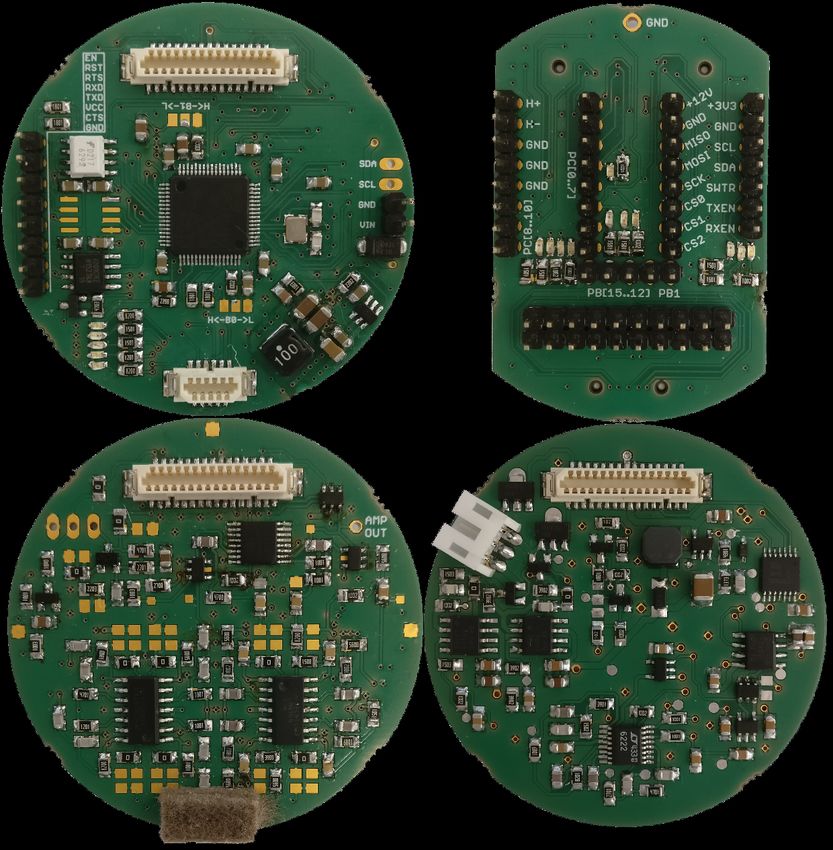
16. GI/ITG KuVS Fachgespräch
                         Sensornetze

                 der GI/ITG Fachgruppe
            Kommunikation und Verteilte Systeme

             07.-08. September 2017 in Hamburg

                            Organisation

General Chair
Karl-Ragmar Riemschneider
Thomas Schmidt

Technical Program Commitee
Falko Dressler
Christian Renner
Bettina Schnor
Lars Wolf

Organizational (Publication, Local Arrangements, Social Event)
Peter Kietzmann
Valentin Roscher
Thorben Schüthe
Preface

Welcome to Hamburg and welcome to FGSN’17, the 16th edition from the series
of GI/ITG KuVS events on Wireless Sensor Networks and the Internet of Things.
It is a great pleasure to host this community event and provide an open atmo-
sphere for new ideas and discussions, demonstrations and exchange–finally a pro-
fessional environment for maintaining the kicker tradition introduced by Georg
Wittenburg 2008 in Berlin.

As traditional in the field, this year’s program reflects the multifaceted works
about constrained nodes and their wireless communication. Various experiments
and implementations tackle these challenges in a lively manner. With the advent
of complex IoT solutions, though, aspects of system and data management came
closer into focus. Here, we are particularly happy about a lightening talk by
Gabe Rodriguez (Google) on Google’s IoT strategy. On the overall, we have to
emphasize our gratitude to the program team Falko Dressler, Christian Renner,
Bettina Schnor, and Lars Wolf, who managed to assemble a convincing program.

FGSN’17 would not have been possible without our efficient organising team:
We are very grateful to Peter Kietzmann, Valentin Roscher, and Thorben Schüthe
for their fantastic job on everything that was needed. We also thank the ’Förder-
verein Elektrotechnik und Informatik der HAW Hamburg e.V.’ for the generous
support of this event.

We hope you all will enjoy two days of exchange and inspiration in the beautiful
city of Hamburg!

Karl-Ragmar Riemschneider &
Thomas C. Schmidt &
FGSN’17 Chairs
Contents

Session 1: Protocols and Reliability
  miniDTN: A DTN Stack for 5-WiFi-Nodes . . . . . . . . . . . . . . . . . . . . . . . . . . . . . . . .               1
  Stephan Rottmann, Alexander Willecke, Jan äberich, Georg von Zengen and Lars Wolf
  End-to-End Performance Analysis for Industrial IEEE 802.15.4e-based Networks . . . . . . .                          5
  Neda Petreska
  Improving MAC Layer Reliability Through Interference-Adaptive TSCH Cell Assignment .                                9
  Leo Krüger, Lotte Steenbrink and Andreas Timm-Giel

Session 2: Network Performance and Management
  Stop Waiting: Mitigating Varying Connecting Times for Infrastructure WiFi Nodes . . . . . 13
  Lars Hanschke, Jan Heitmann and Christian Renner
  Einfluss der Gradverteilung bei Multicast Growth Codes . . . . . . . . . . . . . . . . . . . . . . . 17
  Isabel Madeleine Grimm and Reiner Kolla
  Managing IoT device capabilities based on oneM2M ontology descriptions . . . . . . . . . . . . 23
  Kristina Sahlmann, Thomas Scheffler and Bettina Schnor

Session 3: Energy Measurement and Consumption
  Ein Leistungsmesssystem für verteilte Sensorknoten zur Unterstützung bei der Implemen-
      tierung von Protokollen in WSN . . . . . . . . . . . . . . . . . . . . . . . . . . . . . . . . . . . 27
  Max Frohberg and Mario Schölzel
  TUCap: A Sensing System to Capture and Process Appliance Power Consumption in Smart
      Spaces . . . . . . . . . . . . . . . . . . . . . . . . . . . . . . . . . . . . . . . . . . . . . . . . . . . . 31
  Andreas Reinhardt
  Eine Testplattform für Energy Harvesting mit RIOT . . . . . . . . . . . . . . . . . . . . . . . . . 35
  Michel Rottleuthner and Thomas C. Schmidt

Session 4: Heterogeneous Communications
  Kommunikation in heterogenen Sensornetzwerken mittels Cross-Plattform und Multiradio-
       Gateways . . . . . . . . . . . . . . . . . . . . . . . . . . . . . . . . . . . . . . . . . . . . . . . . . . 39
  Paul Poppe, Sebastian Reinhold, Danny Puhan, Max Frohberg and Mario Schölzel
  About Deployment Limitations of LoRa Gateways . . . . . . . . . . . . . . . . . . . . . . . . . . . 43
  Albert Pötsch and Florian Haslhofer
  Evolution of an Acoustic Modem for AUVs . . . . . . . . . . . . . . . . . . . . . . . . . . . . . . . 47
  Jan Heitmann, Lucas Bublitz, Timo Kortbrae and Christian Renner

Session 5: Position Detection
  Challenges for Sensor Network Based Outdoor Positioning in Forests - A Case Study . . . . 51
  Silvia Krug and Jochen Seitz
  Using Wireless Sensor Networks for Object Location and Monitoring . . . . . . . . . . . . . . . 55
  Frank Senf, Silvia Krug and Tino Hutschenreuther

Posters & Demos
  Contributions . . . . . . . . . . . . . . . . . . . . . . . . . . . . . . . . . . . . . . . . . . . . . . . . . . . 59
FGSN2017

         miniDTN: A DTN Stack for 5C-WiFi-Nodes
              Stephan Rottmann, Alexander Willecke, Jan Käberich, Georg von Zengen, and Lars Wolf
                                        Institut für Betriebssysteme und Rechnerverbund
                                                    TU Braunschweig, Germany
                           Email: [rottmann | willecke | kaeberic | vonzengen | wolf]@ibr.cs.tu-bs.de

   Abstract—Deployments of wireless networks consisting of small                                                  Application
nodes offer many possibilities in the fields of Internet of Things        Storage
(IoT), smart farming applications or Body Area Networks. To
cope with implied challenges like low energy resources, failing           Routing                                    Agent
links, limited computation power and many more, a robust
communication stack is beneficial. An example for such a stack
                                                                         Discovery
is the Delay/Disruption Tolerant Networking (DTN) architecture.
   In many cases, the sensor nodes consist of extreme low power
nodes, 8 bit controllers. However, for several applications, more                         Convergence Layer
resources would be beneficial, at least for some components of            Ethernet      802.15.4       LoRa          802.11
the networks. In this paper, we focus on more powerful systems,
such as 32 bit controllers bridging the gap between traditional          MAC/PHY       MAC/PHY        MAC/PHY       MAC/PHY
Wireless Sensor Networks and PCs. We present miniDTN, a DTN
implementation based on FreeRTOS for many kinds of nodes,                       Fig. 1: Architecture of miniDTN stack
enabling communication via different media, such as Ethernet,
WiFi or LoRa.
                                                                     these boards, DTN becomes suitable to applications where
                      I. I NTRODUCTION                               traditional Wireless Sensor Network (WSN)-nodes were not
                                                                     powerful enough and PCs were not affordable, like gathering
   Wireless sensor and actuator networks can be useful for a         vast amounts of data in smart farming applications. To be
vast amount of applications. They can be used in structural          able to exploit the capabilities of these boards, we developed
health monitoring of buildings, for home automation purposes         miniDTN, based on µDTN [5].
or in the field of smart farming as well as the Internet of             An example smart farming application and use case has
Things (IoT). Depending on the actual use case of a network          been presented in [7], [8]. The task of the sensor network is
installation, the amount of nodes deployed may also vary. The        to collect data about temperate and soil humidity on a field
more nodes are deployed, the higher the probability of failures      and forward this data when a tractor is working on that field
will be. Nodes may disappear from the network due to power           is passing by to a mobile node. After the tractor returns to the
failures resulting from empty batteries, software errors or radio    farm, it forwards this data to a sink node, where it might be
interference.                                                        processed or stored in any kind of database.
   Being able to cope with these problems, a robust communi-            In Section II, we describe in more detail how miniDTN
cation protocol is necessary to ensure high reliability for data     works and what its architecture looks like. The platforms we
transmissions – even if some nodes fail.                             target with miniDTN and what their features are is pointed out
   A robust communication approach for networks, which may           in Section III. To show which applications can benefit from
have unreliable links due to mobility or shortage of energy, is      miniDTN, we perform an evaluation and discuss the results in
the Delay/Disruption Tolerant Networking (DTN) architecture          Section IV. Section V concludes the paper.
[1], [2]. Moreover, DTN is actually able to benefit from node
mobility by storing packets – in DTN called bundle – on                                   II. A RCHITECTURE
the node and physically carrying them to another location               In miniDTN the agent – shown in Fig. 1 – is the central
before forwarding them. Several implementations targeting a          instance which coordinates all the other components shown.
broad range of platforms exist (ION-DTN [3], IBR-DTN [4],            As we implemented miniDTN for FreeRTOS, the agent is
µDTN [5], JDTN, ByteWalla, µPCN [6], DTN2, . . . ). Only             the part to be launched from the FreeRTOS environment.
few of them can be used on very “small” systems like an 8 bit        Modules are shown as blocks in Fig. 1. Each of them is
microcontroller, while others are designed for full-featured         responsible for one major task within miniDTN. The modules
operating systems like Linux running on PCs.                         are: Storage, Routing, Discovery and Convergence Layer. The
   During the last years, more and more relatively cheap,            coordination between the different modules is event driven,
but powerful hardware platforms emerged on the market.               thus expanding or exchanging modules is eased. That comes
Examples are 32 bit ARM controllers and their development            in handy if an application has special routing needs or a
boards or the ESP32, a dual-radio WiFi node running at               platform offers a specialized kind of storage. For most modules
up to 240 MHz with two cores. Due to the low price of                only one implementation is allowed at compile time. The only

                                                                 1
FGSN2017
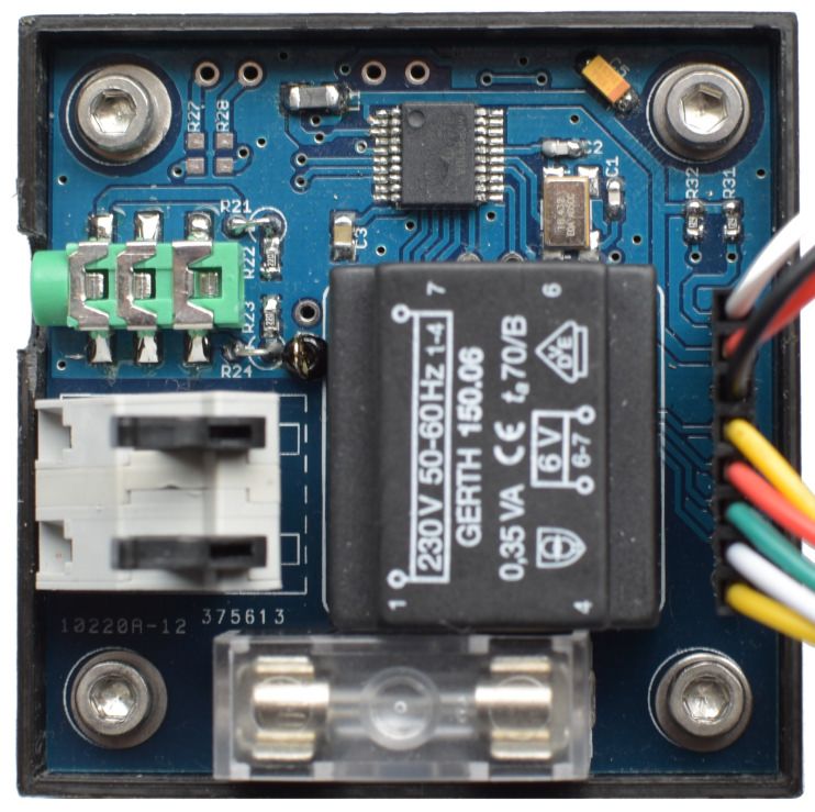
(a) ESP32 with IEEE 802.15.4 radio (b) STM32F4Discovery (c) Amphisbaena
Fig. 2: Different platforms currently supported by miniDTN
exception is the Convergence Layer (CL). Depending on the between networks using different communication mediums.
platform, multiple CLs can be loaded, using different kind of Another application is the use of different wireless standards
communication interfaces. for according tasks, e.g. using a low power standard for
• Application: To use the DTN stack, the user needs heartbeats and smaller bundles and IEEE 802.11 for large
to write an application which registers an endpoint at bundles. Fig. 2b shows the well-known STM32F4Discovery
the agent. Bundles received for this endpoint are made board with an Ethernet shield. Amphisbaena uses the same
accessible for the application. central hardware components and thus, the performance of
• Agent: The agent is the central process started on the both is the same.
actual platform from the user code. It manages the miniDTN can be ported to any other hardware where
interaction of the other components. FreeRTOS is available. It is open source and available in a
• Storage: The storage module’s task is to make received GIT1 repository. For Ethernet and WiFi communication, the
or generated bundles accessible for the application or LwIP stack in version 2.0.0 is used.
routing. Bundles may be stored in the microcontroller’s For the mentioned platforms, examples are present on-
RAM or on a SD card in the FAT file system, for example. line2 . It also runs on commonly available ESP32 develop-
The latter one is slower but bundles are stored nonvolatile ment boards. To use the implementation in a new project,
and thus are still available after a reset. the miniDTN code needs to be added to the build-system.
• Routing: The routing module decides which bundles Low level definitions for the hardware interface have to be
should be sent to which neighbors. A simple flooding configured in a single header file.
forwards bundles to all nodes except the originating one. IV. P ERFORMANCE E VALUATION
• Discovery: The discovery part of the implementation
keeps track of the neighbors and their convergence layers. In smart framing applications, networks in the farm itself
Beacons are sent out announcing nodes on a broad- or consist of stationary nodes like servers or workstations. These
multicast channel of the actual medium. By now, we nodes are typically connected via IEEE 802.3. Additional
implemented a DTN IP Neighbor Discovery (IPND) [9] network nodes might be used to monitor either the storage of
conform mechanism. the crop, for example. As a farm often is spread over a large
• Convergence Layer: In miniDTN, multiple CLs can be
area, wireless and mobile nodes might be used to connect the
implemented. At the moment dgram:udp for commu- wired networks with each other by physically carrying bundles
nication in IP networks as well as dgram:lowpan for using mobile nodes such as tractors. The use of wireless nodes
transfers via IEEE 802.15.4 or LoRa are available. The is not limited to carry bundles, they can also be used to monitor
two latter ones are using the same frame format, only the cattle and plants on the fields. In our evaluation we will show
radio driver needs to be modified. The TCPCL [10] is in that miniDTN is suitable for all these applications.
development. To do so, we evaluated a minimal setup shown in Fig. 3.
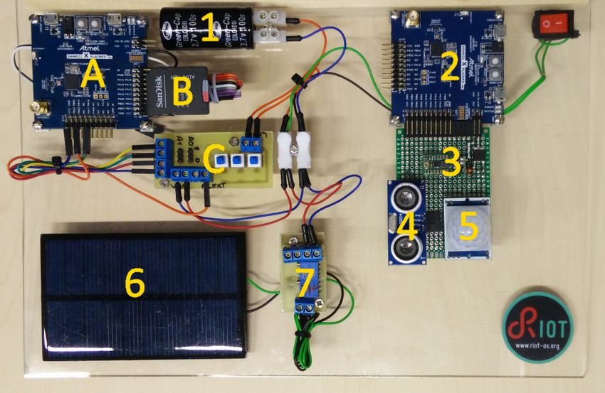
A router running OpenWRT is used to connect all nodes:
III. TARGET P LATFORMS • Raspberry Pi: A PC style node based on a Raspberry
Pi 3 running IBR-DTN on Linux. It uses the integrated
We have different target platforms shown in Fig. 2, which
WiFi device to connect to the AP.
miniDTN is ported to. Fig. 2a is an ESP32 on a development
• Amphisbaena: The low-power-part of our dual-platform
board with a pluggable Atmel AT86RF233 radio. Thus, it
node Amphisbaena, connected via Ethernet. It is based
is able to communicate via IEEE 802.11b/g/n as well as
on the same components as the STM32F4Discovery.
IEEE 802.15.4 or LoRa. Fig. 2c is our Amphisbaena platform
[11], which is also able to carry different types of wireless 1 https://gitlab.ibr.cs.tu-bs.de/minidtn/minidtnStack
transceivers. That way these platform might work as a bridge 2 https://gitlab.ibr.cs.tu-bs.de/minidtn
2FGSN2017
Raspberry Pi Next, the goodput is evaluated between the platforms using
WiFi Router
802.11
different communication links. The goodput is defined as the
802.3 Amphisbaena
bundle payload size, i.e., the data actually generated by the
802.11 ESP32 application. The evaluation took place in an university lab
environment. This means, that many other WiFi stations exist
ESP32 with SoftAP causing interference. In a real world scenario, this would
be the case, too, depending on the density of nodes in the
Fig. 3: Evaluation Setup for UDP: Continuous lines depict
deployment.
Ethernet, the dashed ones IEEE 802.11n. All node can com-
The results are shown in Fig. 5 (using UDP in IP networks)
municate via IEEE 802.15.4 with each other as well.
and Fig. 6 (for IEEE 802.15.4). In both figures the three
graphs show the goodput to be achieved when sending data
• ESP32: An ESP-WROOM-32 based platform. to a platform. This representation is used to point out the
• ESP32 with SoftAP: The same as before, but not con- differences in the architectures. The platforms ESP32 and
nected to the AP, since it opens its own AP. Amphisbaena are running the code base on microcontrollers.
For the former one, some overhead exists from the SDK which
Thus, the Amphisbaena can be seen as a stationary device and
cannot be influenced by the programmer; it manages the WiFi
the ESP32 acts as a wireless node. Both are using the same
interface, for example.
code base of miniDTN. All our evaluations are done within
Due to the rather small amount of RAM available on the
this setup, all nodes use IPND to discover their neighbors,
microcontroller based platforms, a bundle size larger than
flooding routing to find the route – which in our case is
8 kByte will become unfeasible, since the whole bundle has
always the next hop – and the bundles are transferred using
to be kept in the memory for processing.
the dgram:udp CL. As storage we use the RAM module to
In Fig. 5a to Fig. 5c, we can see that when the dgram:udp
get the best performance in our measurements.
CL is used, the goodput which can be achieved is strongly
A. Results dependent on the bundle’s payload size and the combination of
nodes. Fig. 5c reveals that the performance decreases as soon
To show how long a contact between two nodes needs to last
as a bundle does not fit into the MTU of an Ethernet or WiFi-
until data is transmitted, we measured the time between power-
frame when sending data to IBR-DTN. When sending bundles
on and the first bundle transmission. This includes the boot
with a payload size of 1024 Byte, 300 kByte/s to 600 kByte/s
process, the network configuration and the time the discovery
can be achieved, but at a payload size of 2048 Byte, it drops
takes to discover neighboring nodes, we call this time start-up
to less than 100 kByte/s. The difference between the source
time. Fig. 4 shows the start-up time for the Amphisbaena and
nodes (Amphisbaena vs. ESP32) results from the fact that the
the ESP32. We did not test the start-up time for the Raspberry
Amphisbaena is connected via Ethernet to the AP, and thus
Pi, as such PC like devices take a lot longer to boot and as
only one WiFi link is used. The same effect can be observed
servers they are running most of the time, anyways.
when looking at Fig. 5a. If one of the ESP32 creates a software
For the Amphisbaena we measured a maximum start-up
AP, the data has to be sent only once over the air, and not to
time of 3.2 s, the ESP32 needs with 8.9 s a lot longer. This is
the external AP which transmits the data to the second ESP32.
due to the WiFi association process that the Amphisbaena does
Fig. 6a to Fig. 6c show the same evaluation setup as before,
not need. These result show that a contact time of 10 seconds
but for the use of IEEE 802.15.4. As expected, the goodput
is sufficient to transfer data.
is much lower since the data rate of the physical layer is
The 3.2 s of the Amphisbaena give an idea how much a
only 250 kBit/s. When sending data to miniDTN, only around
stationary device can be duty cycled to save energy and put
12 kByte/s can be achieved, while IBR-DTN is able to accept
the node into a deep sleep mode.
data with around twice the speed – as long as bundles are
not larger than 2 kByte. For larger bundles, the performance
decreases to a similar level as when sending data to miniDTN.
8 Using IEEE 802.15.4 consumes less energy than WiFi. If
only small amounts of data (like heartbeats or temperature
Start-up time in s
6 values) should be transmitted by nodes deployed in the field,
the low power link should be chosen. Data can be aggregated
4
and transmitted in once in large bundles via WiFi, which can
be turned on for example, when a mobile node arrives. The
presence of such a node can be detected via the low power
2
link.
ESP32 Amphisbaena
V. C ONCLUSION
Fig. 4: Comparison of start-up time between the ESP32 and In this paper, we presented miniDTN, a DTN implemen-
Amphisbaena. tation based on FreeRTOS, running on many different kinds
3FGSN2017
300 To ESP32, UDP 400 To Amphisbaena, UDP 700 To IBR-DTN, UDP
From ESP32, SoftAP From ESP32, Ext. AP From ESP32, Ext. AP
350 600
250 From ESP32, Ext. AP From IBR-DTN From Amphisbaena
From IBR-DTN, Ext. AP 300
500
200 From Amphisbaena, Ext. AP
Goodput (kByte/s)
Goodput (kByte/s)
Goodput (kByte/s)
250
400
150 200
300
150
100
200
100
50
50 100
0 0 0
16 32 64 128 256 512 1024 2048 4096 8192 16 32 64 128 256 512 1024 2048 4096 8192 16 32 64 128 256 512 1024 2048 4096 8192
Payload Size (Byte) Payload Size (Byte) Payload Size (Byte)
(a) (b) (c)
Fig. 5: Measurements with UDP over WiFi/Ethernet
14 To ESP32, IEEE 802.15.4 14 To Amphisbaena, IEEE 802.15.4 30 To IBR-DTN, IEEE 802.15.4
12
12 25
10
10 20
Goodput (kByte/s)
Goodput (kByte/s)
Goodput (kByte/s)
8
8 15
6
6 10
4
From ESP32
From IBR-DTN 4 From ESP32 5 From ESP32
2
From Amphisbaena From IBR-DTN From Amphisbaena
0 2 0
16 32 64 128 256 512 1024 2048 4096 8192 16 32 64 128 256 512 1024 2048 4096 8192 16 32 64 128 256 512 1024 2048 4096 8192
Payload Size (Byte) Payload Size (Byte) Payload Size (Byte)
(a) (b) (c)
Fig. 6: Measurements with IEEE 802.15.4
of platforms. Common platforms are already supported, while [4] S. Schildt, J. Morgenroth, W.-B. Pöttner, and L. Wolf, “IBR-DTN: A
it can be ported to any custom board, supporting FreeRTOS. lightweight, modular and highly portable Bundle Protocol implementa-
tion,” Electronic Communications of the EASST, vol. 37, pp. 1–11, Jan
The evaluation has shown that it is able to transfer sufficient 2011.
amounts of data in rather short contacts. Especially if the speed [5] G. von Zengen, F. Büsching, W.-B. Pöttner, and L. Wolf, “An Overview
of tractors while field work and the amount of data gathered of µDTN: Unifying DTNs and WSNs,” in Proceedings of the 11th
GI/ITG KuVS Fachgespräch Drahtlose Sensornetze (FGSN), Darmstadt,
is taken into account. Germany, 9 2012.
When using dgram:udp, the bundles containing the data [6] M. Feldmann and F. Walter, “upcn: A bundle protocol implementation
to be transferred should be chosen as large as possible to for microcontrollers,” in 2015 International Conference on Wireless
Communications Signal Processing (WCSP), Oct 2015, pp. 1–5.
achieve the best goodput, however when sending data to IBR- [7] B. Gernert, S. Rottmann, and L. C. Wolf, “Poster: PotatoMesh - a solar
DTN, the performance decreases significantly as soon as the powered WSN testbed,” in The 17th ACM International Symposium on
MTU of Ethernet or WiFi is exceeded. All in all, one can Mobile Ad Hoc Networking and Computing: MobiHoc 2016 - Posters
(ACM MobiHoc 2016 - Posters), Paderborn, Germany, Jul. 2016, pp.
expect a goodput of at least 150 kByte/s to 200 kByte/s, which 391–392.
is sufficient for the applications targeted by the presented [8] U. Kulau, S. Schildt, S. Rottmann, B. Gernert, and L. Wolf, “Demo:
platforms. Potatonet – robust outdoor testbed for wsns: Experiment like on your
desk. outside.” in Proceedings of the 10th ACM MobiCom Workshop on
R EFERENCES Challenged Networks, ser. CHANTS ’15. New York, NY, USA: ACM,
2015, pp. 59–60.
[1] K. Scott and S. Burleigh, “Bundle Protocol Specification,” RFC 5050 [9] D. Ellard, R. Altman, A. Gladd, and D. Brown, “DTN IP
(Experimental), Internet Engineering Task Force, Nov. 2007. [Online]. Neighbor Discovery (IPND),” Nov. 2015. [Online]. Available:
Available: http://www.ietf.org/rfc/rfc5050.txt http://tools.ietf.org/pdf/draft-irtf-dtnrg-ipnd-03.pdf
[2] V. Cerf, S. Burleigh, A. Hooke, L. Torgerson, R. Durst, K. Scott, [10] M. Demmer, J. Ott, and S. Perreault, “Delay-Tolerant Networking
K. Fall, and H. Weiss, “Delay-Tolerant Networking Architecture,” RFC TCP Convergence-Layer Protocol,” RFC 7242, Jun. 2014. [Online].
4838 (Informational), Internet Engineering Task Force, Apr. 2007. Available: https://rfc-editor.org/rfc/rfc7242.txt
[Online]. Available: http://www.ietf.org/rfc/rfc4838.txt [11] S. Rottmann, R. Hartung, J. Käberich, and L. C. Wolf, “Amphisbaena:
[3] S. Burleigh, “Interplanetary Overlay Network: An Implementation of the A Two-Platform DTN node,” in The 13th International Conference on
DTN Bundle Protocol,” in 2007 4th IEEE Consumer Communications Mobile Ad-hoc and Sensor Systems (MASS 2016) (MASS 2016), Brasilia,
and Networking Conference, Jan 2007, pp. 222–226. Brazil, Oct. 2016.
4FGSN2017
End-to-End Performance Analysis for Industrial
IEEE 802.15.4e-based Networks
Neda Petreska
Fraunhofer Institute for Embedded Systems and
Communication Technologies ESK
neda.petreska@esk.fraunhofer.de
Abstract—In this extended abstract we present an analytical performance of wireless networks was presented in [5]. The
solution for the end-to-end delay bound for multi-hop IEEE so called (min, ×) algebra provides analytical tools to define
802.15.4e-based networks. We base our derivation on the stochas- the bound on the delay violation probability over a cascade of
tic network calculus principles in order to provide performance
guarantees for wireless industrial sensor networks. We validate wireless fading channels.
the derived solution by simulations. Further, we show that the As we are interested in wireless industrial sensor networks
bound is convex, which, together with its monotonicity in the based on the IEEE 802.15.4e standard for low power wireless
average SNR on the links, enables design of algorithms for networks, while at the same time considering queuing effects,
optimal transmit power allocation. These two aspects: optimizing
we present in this work a closed-form solution for the end-
network operation while at the same time providing end-to-end
delay guarantees, are of great importance for the development of to-end delay bound as a performance metric. After a short
reliable, stable and power-efficient wireless industrial networks. discussion of related work in Sec. II and a brief presentation
on the system model in Sec. III, we give an overview of the
used stochastic network calculus and in Sec. IV present the
I. M OTIVATION end-to-end delay bound for IEEE 802.15.4e-based networks.
In Sec. V we discuss the numerical results and conclude the
The fast installation and easy maintenance of wireless paper with upcoming future work.
sensor networks (WSN) makes them suitable for many indus-
trial applications, such as process automation, monitoring and II. R ELATED W ORK
control, predictive maintenance, localization and navigation,
smart grid, logistics and the Internet-of-Things. One of the Many research papers address performance evaluation of
main purposes of these networks, having in mind low-power 802.15.4-based networks, often opting for simulation and/or
battery-driven sensor devices, was to enable an energy-efficient real test-bed evaluation and measurements [6]–[8]. However,
network operation, thereby maximizing their battery lifetime there are not many works presenting analytical approaches for
[1]–[3]. In order to bridge larger distances, especially useful network performance of industrial wireless systems. [9] and
for the application areas of process automation, logistics, local- [10] address performance aspects of IEEE 802.15.4e networks.
ization and navigation of autonomous vehicles, but at the same While [9] provides only simulation experiments to show the
time avoid using significantly higher transmit power which typical operation of the protocol, [10] analytically derives the
would potentially lead to faster battery depletion, multi-hop worst-case latency for typical industrial settings. However, the
communication should be used. However, with the increased latter paper neither considers multi-hop communication nor
industrial digitalization within ”Industry 4.0”, it becomes nec- it involves the queuing delay, i.e., the random capacity of
essary that WSN enable not only an energy-efficient operation, the wireless channel. [11] analyzes the performance of IEEE
but also provide a stable and reliable communication platform 802.15.4e DSME-enabled (Deterministic and Synchronous
for an uninterrupted operation of factory sites and automation Multi-Channel Extension) and IEEE 802.15.4 beacon-enabled
processes. Hence, a set of QoS requirements, mainly given by WSN under the influence of heterogeneous devices. However,
a target delay and packet error rate (PER), have to be met. no analytical framework is presented: the analysis is done
In order to design WSN properly so that the requested rather via simulations. The authors of [12] focus on the
performance of the network is guaranteed, a solid performance network formation process in IEEE 802.15.4e TSCH networks
analysis framework is needed. The challenge of such analysis and analyze the time needed by a node to join the network.
lies obviously in the stochastic nature of the wireless fading They define a random-based advertisement algorithm and
channel. Due to the random wireless channel capacity, queuing evaluate its sensitiveness to different parameters, such as the
effects have to be considered in addition. Such appropriate number of used channel offsets, node density, packet error rate
theoretical framework which enables performance analysis of and number of available frequencies. None of the mentioned
wireless multi-hop sensor networks is the theory of stochastic works presents end-to-end performance analysis for IEEE
network calculus [4]. A recent alternative approach for mod- 802.15.4e networks under queuing aspects due to the random
eling the impact of channel gain models on the network-layer nature of wireless fading channels.
5FGSN2017
III. P RELIMINARIES the allocated time slot and changes from one slotframe to the
In this section we first give a brief introduction to IEEE other. Since two consecutive transmissions by the same node
802.15.4e and then describe the considered system model. on the same link are several time slots apart and potentially
taking place on different channels, the instantaneous SNR of
A. Introduction to the IEEE 802.15.4e Standard the same link are independent and uncorrelated.
The IEEE 802.15.4e standard was designed as an exten- In the following we are going to define a bound on the delay
sion of the CSMA/CA-based IEEE 802.15.4 standard [13] in violation probability. The QoS requirements of the application
order to address the emerging needs of wireless industrial are given with the target delay w and the target probability for
applications. This standard describes a MAC protocol for its violation ε. Hence, we seek to design the WSN in such way,
low-power multi-hop wireless networks, intended to increase such that the delay bound is always smaller than ε.
the reliability and decrease the delay of the network. A
special feature of the standard is the TSCH mode (Time IV. E ND - TO -E ND IEEE 802.15.4 E - BASED D ELAY B OUND
Synchronized Channel Hopping), which is especially targeted As already mentioned, we aim towards a closed-form ex-
to process automation applications. This is why there is a pression of the end-to-end delay violation probability (or also
big similarity between the TSMP (Time Synchronized Mesh called a delay bound) for the multi-hop path presented in the
Protocol) [14], a part of the WirelessHART standard for previous section. We first derive the delay bound for link j. For
process automation and the TSCH. The main reliability-boost this purpose we use the (min, ×) stochastic network calculus
feature lies in the so called slotframes, which represent a in the SNR domain [5] and compute the Mellin transform
time slot to channel matrix. A (time slot, channel) pair is of the arrival and service process. Assuming an industrial
allocated to each transceiver, enabling reduced interference automation application with a constant data rate, we define
between subsequent transmissions. Having a time slot length the cumulative arrival process and its Mellin transform as
of 10 ms, TSCH provides an increased network capacity, high Aj (τ, t) = era (t−τ ) and MAj (s, τ, t) = era (t−τ )(s−1) , s > 0,
reliability and predictable latency. Due to this mode, IEEE respectively. The instantaneous service of the j-th link in the
802.15.4e is especially suited for multi-hop communication, i-th slotframe is Bernoulli distributed:
since neighbouring nodes can be allocated different resources (
within the same slotframe, without interfering with each other. ka , 1 − P(γi,j )
While the slotframes can be of different length, the total Xi,j = (1)
0, P(γi,j )
number of available channels for frequency hopping is 16.
where P(γi,j ) is the probability of erroneously received frame
B. System Model
at link j in slotframe i. The frame error rate is a function of the
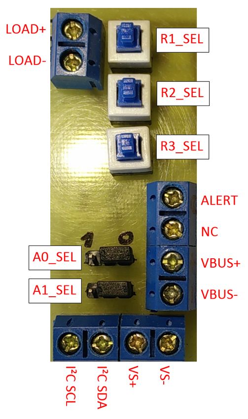
We consider a data flow originating from node a, being BER p(γi,j ), which, in turn, is a function of the instantaneous
forwarded via a cascade of wireless links all the way to a SNR. The cumulative service in the SNR domain results in
destination node b (see Figure 1). At the beginning of each
t−1
Y
slotframe, the application running on a produces payload of Pt−1
Xi,j
Sj (τ, t) = e i=τ = eXi,j . (2)
size ra bits. Several payload packets can be transmitted within
i=τ
a MAC frame of size ka = 127 B. Due to the CRC, the
instantaneous service of each wireless link is a Bernoulli Hence, its Mellin transform is as follows:
distributed random variable and takes values of either 0 or
ka . In case of an unsuccessful transmission, i.e., no reception (t−τ )
of an ACK within a time slot, the packets are being queued MSj (τ,t) (s) = MeXi,j (s)
(3)
at the nodes. Assuming a round-robin scheduling, each node = 1 + (eka (s−1) − 1)Pr(Xi,j = ka ) ,
transmits its buffered packets within the next slotframe, having
one time slot assigned for transmission per slotframe. where Pr(Xi,j = ka ) is the marginal probability distribution
given by:
Z ∞
1 −y
Pr(Xi,j = ka ) = (1 − p(y))ka · e /γ̄j dy, (4)
0 γ̄j
a b for a Rayleigh fading channel and exponentially distributed
SNR with parameter γ̄j .
According to the (min, ×) network calculus, the delay
Fig. 1: Ilustration of the multi-hop path considered in the system
model. The intermediate nodes can queue the packets, in case of an bound K(s, −w) is defined as a function of the Mellin
unsuccessful transmission. transform of the cumulative arrival and service process:
min(τ,t)
We assume block-fading channels, where the instantaneous X
K(s, −w) = MA (1 + s, i, t)MS (1 − s, i, τ ). (5)
SNR of link j at slotframe i, γi,j remains constant during
i=0
6FGSN2017
We are interested in the delay bound for a steady state network,
so we solve Eq. (5) for t → ∞ and obtain: 100
w SNR=[4] dB
SNR=[4, 6] dB
1 + (e−ka s − 1)Pr(Xi,j = ka ) SNR=[4, 6, 8] dB
K(s, −w) = . (6) 10-1 SNR=[4, 6, 8, 5] dB
1 − era s (1 + (e−ka s − 1)Pr(Xi,j = ka )) SNR=[4] dB Sim.
Delay Violation Probability
SNR=[4, 6] dB Sim.
The sum converges if SNR=[4, 6, 8] dB Sim.
SNR=[4, 6, 8, 5] dB Sim.
10-2
era s 1 + (e−ka s − 1)Pr(Xi,j = ka ) < 1, (7)
which at the same time presents the system stability condition. 10-3
Hence, we obtain the delay bound over a link j for a given
target delay w. We encourage the interested reader to take
a look at the whole derivation of the IEEE 802.15.4e-based 10-4
delay bound in [15].
The end-to-end delay bound is obtained from Theorem 1 10-5
in [16], which essentially reveals its recursive nature. The 0 50 100 150 200 250 300 350 400 450 500
Delay [ms]
recursion is especially useful for packet routing and estab-
lishing of new routes in case one link is added to the path Fig. 2: Validation of the delay bound for a IEEE 802.15.4e-based
or a pre-existing link’s average SNR has been changed. In system for different multi-hop scenarios.
such cases, using the recursion to compute the new end-to-end
service curve, saves a lot of computation time in comparison
100
to performing the end-to-end (min, ×) convolution.
V. N UMERICAL R ESULTS 10-2
In this section we show the validity of the obtained ana-
Delay Violation Probability
10-4
lytical delay bound and discuss its properties. Fig. 2 shows
that the end-to-end delay bound is indeed an upper bound on
10-6
the delay violation probability obtained for a IEEE 802.15.4e-
based multi-hop path obtained by simulations. In each iteration 10-8
i of the simulation an instantaneous frame error rate P(γi,j )
is computed, according to the instantaneous SNR γi,j on the 10-10
links along the path. The instantaneous service per link is SNR=[2, 4, 6] dB
drawn from a Bernoulli distribution with this probability. The 10-12
SNR=[5, 7, 9] dB
SNR=[8, 10, 12] dB
packets are propagated in a round robin fashion along the SNR=[11, 13, 15] dB
path and are buffered at the nodes each time Xi,j = 0. We 10-14
0 20 40 60 80 100 120
show the simulated and analytical delay violation probability Delay [ms]
for several target delays and observe that the tightness of the
Fig. 3: Analytical delay bound vs. different target delays for several
bound depends on the number of links of the path. This gap
3-hop scenarios. Doubling the SNR per link leads to two orders of
results from the union bound used in the derivation of the magnitude lower delay bound for payloads of 10 B.
delay bound.
Fig. 3 shows the end-to-end delay bound for several 3-hop
paths, where each path is obtained by doubling the respective the area of process automation, one can design the network
link’s SNR. We observe that the delay bound decreases as the path by enabling SNRs of {5, 7, 9} dB or even lower, which
SNR on the links increases and as the target delay requirement could potentially lead to different node placement or transmit
gets looser. power allocation. Having in mind the approximately one
In Fig. 4 we present a very important characteristic of the order of magnitude gap between the analytical delay violation
end-to-end delay bound obtained by the (min, ×) network probability and the simulated one from Fig. 2, even if the delay
calculus. The bound is convex in s and the minimum of the bound for the path [5, 7, 9] dB lies above ε = 10−3 , the actual
delay bound function depends on the SNR allocation on the system delay violation probability will lie below ε. Allowing
links. As the average SNR on the links is decreased, the min- a lower transmit power is a very important aspect for WSN,
imum is shifted to the left and up. Note here that, every path since this leads to an extended battery and therefore, network
has a different interval for the s parameter, i.e. s ∈ (0, smax ), lifetime. Note that a target delay of 6 slotframes results into
where (0, smax ) follows from the stability condition given a delay of 180 ms for the observed 3-hop scenarios.
by Eq. (7). This convex behaviour opens the question about
an optimal SNR allocation along the path in order to meet VI. C ONCLUSION AND O UTLOOK
certain target QoS. As we can see in the figure, for a target In this extended abstract we present a closed-form so-
delay violation probability of 10−3 , typical for applications in lution for the end-to-end delay bound over a cascade of
7FGSN2017
even broader perspectives to benefit from it even in case of
10 0 time critical processes.
SNR=[2, 4, 6] dB
SNR=[5, 7, 9] dB
10 -1 SNR=[8, 10, 12] dB R EFERENCES
SNR=[11, 13, 15] dB
[1] H. Long, Y. Liu, Y. Wang, R. P. Dick, and H. Yang, “Battery Allocation
Delay Violation Probability
10 -2 for Wireless Sensor Network Lifetime Maximization Under Cost Con-
straints,” in 2009 IEEE/ACM International Conference on Computer-
10 -3
Aided Design - Digest of Technical Papers, Nov 2009, pp. 705–712.
[2] R. Asorey-Cacheda, A. Garcia-Sanchez, F. Garcia-Sanchez, J. Garcia-
Haro, and F. Gonzalez-Castano, “On Maximizing the Lifetime of Wire-
10 -4 less Sensor Networks by Optimally Assigning Energy Supplies,” Sensors
(Basel), vol. 13, no. 8, pp. 10 219–10 244, August 2013.
10 -5 [3] A. A. Aziz, Y. A. Sekercioglu, P. Fitzpatrick, and M. Ivanovich, “A
Survey on Distributed Topology Control Techniques for Extending
the Lifetime of Battery Powered Wireless Sensor Networks,” IEEE
10 -6 Communications Surveys Tutorials, vol. 15, no. 1, pp. 121–144, 2013.
[4] Y. Jiang, “A Basic Stochastic Network Calculus,” SIGCOMM Comput.
10 -7 Commun. Rev., vol. 36, no. 4, pp. 123–134, Aug. 2006.
0 0.005 0.01 0.015 0.02 0.025 0.03 0.035 [5] H. Al-Zubaidy, J. Lieberherr, and A. Burchard, “Network-Layer Perfor-
s mance Analysis of Multi-Hop Fading Channels,” IEEE/ACM Transac-
tions on Networking (ToN), vol. 24, no. 1, pp. 204–217, Feb 2016.
Fig. 4: The end-to-end delay bound is convex in s. The payload size [6] P. Ferrari, A. Flammini, S. Rinaldi, and E. Sisinni, “Performance
is ra = 10 B, the target delay w = 6 slotframes and ε = 10−3 . Assessment of a WirelessHART Network in a Real-World Testbed,”
in Instrumentation and Measurement Technology Conference (I2MTC),
2012 IEEE International, May 2012, pp. 953–957.
[7] J. Song, S. Han, A. Mok, D. Chen, M. Lucas, M. Nixon, and W. Pratt,
wireless fading channels. The provided performance analysis “WirelessHART: Applying Wireless Technology in Real-Time Industrial
allows for the channel gains along the path to be hetero- Process Control,” in Real-Time and Embedded Technology and Appli-
geneously distributed, having different average SNR on the cations Symposium, 2008. RTAS ’08. IEEE, April 2008, pp. 377–386.
[8] J.-S. Lee, “Performance Evaluation of IEEE 802.15.4 for Low-Rate
links. Based on the BER-to-instantaneous-SNR relation given Wireless Personal Area Networks,” IEEE Transactions on Consumer
in the IEEE 802.15.4e standard, we have first derived a service Electronics, Aug 2006.
curve for such system and afterward analytically defined [9] F. Chen, R. German, and F. Dressler, “Towards IEEE 802.15.4e: A Study
of Performance Aspects,” in 2010 8th IEEE International Conference
the bound on the delay violation probability. We have also on Pervasive Computing and Communications Workshops (PERCOM
shown that the provided solution is an upper bound on an Workshops), March 2010, pp. 68–73.
analogously simulated system behaviour. We further present [10] F. Chen, T. Talanis, R. German, and F. Dressler, “Real-Time Enabled
IEEE 802.15.4 Sensor Networks in Industrial Automation,” in 2009
the convex behaviour of the end-to-end delay bound, opening IEEE International Symposium on Industrial Embedded Systems, July
the way towards determining the optimal average SNR needed 2009, pp. 136–139.
on the links along the path in order to guarantee certain [11] J. Lee and W. C. Jeong, “Performance Analysis of IEEE 802.15.4e
DSME MAC Protocol Under WLAN Interference,” in 2012 Interna-
application delay requirement. The provided results can be tional Conference on ICT Convergence (ICTC), Oct 2012, pp. 741–746.
used in the network design of QoS-driven wireless industrial [12] D. D. Guglielmo, A. Seghetti, G. Anastasi, and M. Conti, “A Perfor-
IEEE 802.15.4e-based networks, such as WirelessHART [17] mance Analysis of the Network Formation Process in IEEE 802.15.4e
TSCH Wireless Sensor/Actuator Networks,” in 2014 IEEE Symposium
and ISA100.11a [18]. on Computers and Communications (ISCC), June 2014, pp. 1–6.
In a previous work [19] we have used the convexity of the [13] IEEE 802.15.4 WPAN Task Group, “802.15.4e-2012: IEEE Standard for
bound in s and the monotonicity in γ̄ and have defined a binary Local and Metropolitan Area Networks - Part 15.4: Low-Rate Wireless
Personal Area Networks (LR-WPANs) Amendment 1: MAC sublayer,”
search algorithm, which determines the optimal transmit power April 2012.
on a single link, in order to meet certain statistical delay [14] K. S. J. Pister and L. Doherty, “TSMP: Time Synchronized Mesh
constraints. However, this was done for a service modeled ac- Protocol,” in IASTED Internatinal Symposium on Distributed Sensor
Networks. Acta Press, 2008, pp. 391–398.
cording to the Shannon capacity. On the other hand, the IEEE [15] N. Petreska, H. Al-Zubaidy, B. Staehle, R. Knorr, and J. Gross, “Statis-
802.15.4e-based service curve and delay bound enable similar tical Delay Bound for WirelessHART Networks,” in Proceedings of the
approach, only this time, for practical wireless industrial 13th ACM Symposium on Performance Evaluation of Wireless Ad Hoc,
Sensor and Ubiquitous Networks. New York, NY, USA: ACM, 2016,
networks. Currently, we are looking into a similar algorithm pp. 33–40.
which would maximize the minimal battery lifetime of the [16] N. Petreska, H. Al-Zubaidy, R. Knorr, and J. Gross, “On the Recur-
nodes along a multi-hop path for a system model as presented sive Nature of End-to-End Delay Bound for Heterogeneous Wireless
Networks,” in IEEE International Conference on Communications 2015
in this paper. Determining the optimal transmit power so that (ICC 2015). London: IEEE, June 2015, pp. 5998–6004.
given end-to-end statistical delay constraints are guaranteed [17] H. C. Foundation, “WirelessHART R Technology,” 2013. [Online].
in a wireless industrial network, will open new perspectives Available: http://www.hartcomm.org/
[18] ISA100 Commitee. (2014) ISA100, wireless systems for automation.
in the design of industrial WSN. Such results would be of [Online]. Available: www.isa.org/isa100
essential meaning for the further development of wireless [19] N. Petreska, H. Al-Zubaidy, and J. Gross, “Power Minimization for
industrial networks, enabling both reliability and flexibility. Industrial Wireless Networks under Statistical Delay Constraints,” in
Teletraffic Congress (ITC), 2014 26th International. Karlskrona: IEEE,
Performance analysis together with optimal resource allocation Sept 2014, pp. 1–9.
in WSN has the potential to enable faster acceptance of
wireless communication for industrial applications and open
8FGSN2017
Improving MAC Layer Reliability Through
Interference-Adaptive TSCH Cell Assignment
Leo Krüger, Lotte Steenbrink and Andreas Timm-Giel
Institute of Communication Networks (ComNets)
Hamburg University of Technology
Email: {leo.krueger,lotte.steenbrink,timm-giel}@tuhh.de
Abstract—Channel hopping and TDMA are often used to interference from nodes outside the network. This Scheduling
avoid interference and thus increase the reliability of Medium Function is a heuristic where nodes autonomously coordinate
Access Schemes in Wireless Sensor Network (WSN). This is the use of (channel, timeslot) resources (so-called
a useful, but blind approach: it minimizes the probability for
(repeated) collisions, but does not actively avoid them. In this cells) according to their local knowledge about interferences
paper, we propose a MAC scheme that is able to predict and on different channels. Therefore, the allocation of cells adapts
adapt to interference, building on existing research in the field to the interference present. In a second step, interference
of Cooperative Spectrum Sensing (CSS). The proposed scheme is prediction is also taken into account.
integrated into IEEE 802.15.4e Time Slotted Channel Hopping Our application scenario incorporates industrial environ-
(TSCH) as a new 6P Scheduling Function, leveraging existing
standards and Internet-Drafts optimized for the deployment in ments in which several hundred mobile IEEE 802.15.4e nodes
Low Power and Lossy Networks (LLNs). are deployed without strict prior planning. Co-located IEEE
802.11 (WLAN) and 802.15.1 (Bluetooth) networks are the
I. I NTRODUCTION main source of interference. It has already been shown that
The demands on Wireless Sensor Networks (WSNs) in IEEE 802.15.4 is affected by such networks. It is expected that
industrial environments are changing. Whereas previous de- the effect is mitigated by channel hopping, but not neutralized
ployments of such networks encompassed mostly uncritical completely [2]. The traffic model is peer-to-peer communica-
applications such as environmental sensing, the focus has tion without any central sink. Among others, it includes time
shifted to use cases with stringent requirements with regard critical applications. The used hardware is equipped with two
to delay and packet loss. Examples for this are control and radios, which allows for parallel spectrum sensing and sending.
monitoring of machinery as well as the usage of a WSN in Nevertheless, single-radio setups are not to be ignored.
networked control loops. For the moment, we aim at reducing delays in a network
To satisfy these requirements, Time Division Multiple with only best-effort service by decreasing the number of
Access (TDMA) and/or channel hopping-based Medium necessary retransmissions. For that, we present an appro-
Access Schemes are used. This helps optimize medium uti- ach where nodes autonomously and dynamically adjust their
lization and avoid packet collision as timeslots are assigned scheduling according to sensed interference. In the future,
only once, but it also introduces delays: First, the allocation additionally guaranteeing application dependent delay bounds
of timeslots defines the time a packet has to wait before it will be the focus of our work.
can be transmitted on the link. This is especially relevant This paper is organized as follows. First, related work is
for nodes forwarding packets, as the receive timeslot of a summarized. In the subsequent section the corresponding pre-
packet is not necessarily close to its forwarding timeslot. requisites such as the Time Slotted Channel Hopping (TSCH)
Second, retransmissions lead to transmission delays which Medium Access Scheme and existing Scheduling Functions
are amplified if the time until the next allocated timeslot is are introduced. In Section IV a novel interference-adaptive
particularly long. Third, non-empty queues on nodes might Scheduling Function is proposed. The paper concludes with an
lead to a queuing delay when either the offered load cannot be outlook on envisioned evaluation methodology and our future
satisfied by the slot allocations or retransmissions lead to more research direction.
timeslots being required. Testbed measurements [1] already
have shown that retransmissions as well as queuing have a II. R ELATED W ORK
significant impact on the delay in networks as considered here. Proposals to mitigate network interference can be catego-
Consequently, delays can be reduced by either optimizing rized into two approaches: channel estimation and spectrum
the slot allocation, e.g. by taking into account the paths sensing.
in the network, their offered load, and an over-provisioning In the former, network characteristics such as the Packet
to cope with a certain amount of retransmissions. Or by Delivery Ratio (PDR) are monitored to filter out channels that
reducing the amount of retransmissions through avoiding inter- negatively affect the network performance. To do this, Mura-
network-interference. In this paper we will focus on the oka et al. Muraoka et al. propose a housekeeping mechanism
latter, presenting a Scheduling Function aimed at avoiding that tracks packet collision rates and relocates affected cells
9FGSN2017
[3], which is a way to mitigate interference without directly
measuring or predicting it. It is also important to note that
cells are assigned randomly on initialization. It is up to the
housekeeping mechanism to improve the initial choice over
time.
In the latter, the spectrum is sensed – either by a dedicated
antenna or in between transmissions – in order to detect and
avoid interferences. Proposals to leverage spectrum sensing for
WSNs can be found. Yoon et al. group nodes into parent-child Fig. 1. TSCH cell assignment.
clusters which switch their shared hopping sequence when an
interference is detected [4]. Du et al. propose A-TSCH [5],
an extension that uses spectrum sensing to detect channels are dedicated to specific nodes at specific times, avoiding
with high noise levels: nodes blacklist either a fixed number collisions. Being able to operate on different channels per
of channels or those that fall below a certain quality threshold. timeslot also expands the amount of available resources. If
Blacklists do not appear to contain information about the all nodes employ different hopping patterns, they will only
channel quality and are distributed among all neighboring briefly be exposed to external interference if it remains on
nodes. Testbed experiments with an unspecified number of one channel of their hopping pattern.
nodes and fixed blacklist sizes (i.e. the N worst channels The original IEEE 802.15.4 standard already defines a
are blacklisted regardless of their overall quality) suggest that mode where timeslots in a star topology are used. Within a
this technique improves the average PDR and stabilizes the superframe the contention free period allows for 7 exclusive
network time synchronization when compared to blind channel timeslots. Since this does not scale well for a higher number of
hopping. nodes and a mode for multi-hop networks is not defined, IEEE
Spectrum sensing for interference avoidance has also been 802.15.4e introduces Time Slotted Channel Hopping (TSCH)
researched extensively in the field of Cooperative Spectrum – a MAC scheme providing the infrastructure for distributed
Sensing (CSS), which is used in Cognitive Radios to enable TDMA channel hopping. However, many parameters such as
Secondary Users (SUs) to use a frequency assigned to a slotframe size and time synchronization intervals as well as
Primary User (PU) when the PU is not active. This is done by the exact joining and negotiation process are not defined by
sensing the medium for any activity from the PU, and stopping the standard. The IETF 6TiSCH Working Group aims to fill
any transmissions. SUs may compare their measurements to this void by standardizing protocols and best practices for the
collaboratively determine whether the PU is actually present use of TSCH with IPv6 in Low Power and Lossy Networks
and predict its future activities. Usually, a dedicated channel (LLNs). Its 6top sublayer defines the 6top Protocol (6P) [11],
is used for control traffic. This is by definition a best-effort which specifies 6P Transactions to negotiate cells for data
service only; the optimization lies in making the channel transmission off the network’s default hopping pattern. Cells
available at all. The collaborative interference measurement are (channelOffset, slotOffset) tuples that mark a
evaluation of CSS is not needed in the scenario at hand – if window in which directed communication between two nodes
one node is experiencing interference, this affects the network, can take place. channelOffset is always relative to the
regardless of who else has similar measurements. default hopping pattern. Fig. 2 illustrates how the 6top sublayer
The intersection between CSS and Interference-Adaptive introduced by 6TiSCH is integrated into the network stack.
Frequency Hopping lies in interference prediction, which has
been discussed more widely in the Cognitive Radio world: A. Scheduling Functions
several authors [6], [7] [8], [9] propose and analyze models 6TiSCH defines Scheduling Functions, which initiate 6P
to predict WLAN interference. For IEEE 802.15.4e networks, Transactions to schedule new cells or reschedule existing ones.
only Vasseur et al. describe a mechanism to exchange pre- They determine which cells (if any) are most suitable for
diction information [10], but the predicted data is mainly all participants. Scheduling Functions can be divided into
changes in the traffic forwarded by the node itself. two categories: interface-based and link-based. The former
assigns channels locally per-interface, while the latter assigns
III. P REREQUISITES dedicated channels to specific transmissions.
Multiple standards specifying Medium Access schemes for So far, two Scheduling Functions have been proposed –
WSNs are already available. Adaptions for the the original Scheduling Function 0 (SF0) [12] and Scheduling Function 1
IEEE 802.15.4 standard MAC and Network layer such as (SF1) [13]. The former is an active Working Group document,
WirelessHART, ISA 100.11a and the IEEE 802.15.4e amend- while the latter is an independent draft. The main difference is
ment have been specified. All of the above support TDMA that SF0 is interface-based and provides a best-effort service
and partially also channel hopping: time-frequency resources where cells are scheduled hop by hop and can be used by
– so-called timeslots – are exclusively assigned to certain multiple links, while SF1 is a link-based Scheduling Function,
communication partners. This helps reduce intra-network in- using the Resource Reservation Protocol (RSVP) to allocate
terference, as traffic is divided over multiple frequencies which the available bandwidth. SF1 is optimized for industrial net-
10FGSN2017
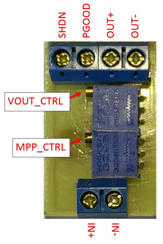
which sweeps all channels for interferences and informs an
Routing
Interference Prediction Mechanism (IPM). If the IDM detects
IPv6 an interference, it notifies SF2 by triggering the Interference
Detected event. SF2 then adds all cells affected by this
6top Sublayer interference in the near future to a blacklist, and triggers a
Scheduling Function rescheduling which moves transmissions currently using the
6p affected cells to different, usable cells.
Interference is not a binary matter, but a question of whether
IEEE 802.15.4e TSCH a channel is noisy enough to disrupt data transmission or
not. Therefore, the blacklisted cells are provided with an
IEEE 802.15.4 PHY interference probability metric which denotes the probability
that a transmission over this cell will be faulty. The same
Fig. 2. TSCH/6top Stack. The proposed Scheduling Function is a part of the goes for predictions: since the IPM cannot always be 100%
6top sublayer, which completes the functionalities provided by TSCH. It uses confident about its predictions, the interference probability
6P for cell negotiation.
metric here refers to the probability that the predicted (critical)
interference actually occurs.
Node A Node B The interference probability metric is also included in the
Available cells: CellList of the 6P transaction process illustrated in Fig. 3. This
[(slotOffset: 1, channelOffset: 2, intfProb: 0.0), way, nodes can find cells that might work for both of them
(slotOffset: 2, channelOffset: 3, intfProb: 0.2),
(slotOffset: 3, channelOffset: 5, intfProb: 0.3)] even in the face of slight interference. Cells whose interference
probability is above a certain threshold are not taken into
6P ADD Request account when negotiating new links with neighbors.
Fig. 3 illustrates the negotiation process for a new set of
NumCells = 1
CellList =
[(slotOffset: 1, channelOffset: 2, intfProb: 0.7), cells: First, node A sends an ADD request which includes
(slotOffset: 2, channelOffset: 3, intfProb: 0.5),
(slotOffset: 3, channelOffset: 5, intfProb: 0.0)]
the interference probability in the CellList, along with the
number of cells to be scheduled (NumCells). Node B then
6P RESPONSE
picks those NumCells cells from the list that have minimal
CellList = [(slotOffset: 3, channelOffset: 5)] interference probability for both sides and communicates its
choice in the 6p response. The cell selection takes into account
6P CONFIRMATION [optional] both the absolute interference probability of both sides as well
CellList = [(slotOffset: 3, channelOffset: 5)] as the difference between them: among those cells with the
lowest interference probability on both sides, pick the cell
with balanced interference probabilities to avoid cases where
Fig. 3. An example 6P Transaction negotiating a cell to use between nodes the interference probability is high on one side while it is low
A and B by including SF2 interference information intfProb as mandated
by SF2.
on the other. In such a case the high probability on one side
most probably leads to a retransmission, either due to a lost
packet or acknowledgment.
works and aims to make hard real-time guarantees, but it Had Node A only communicated the slotOffset and
appears to be in an early stage. channelOffset of its available cells, Node B might have
picked (1, 2), since it is the first entry in CellList and has an
IV. S CHEDULING FUNCTION interference probability intfProb of 0 for Node B. For A,
In order to obtain interference-adaptive cell allocation, a however, this would have been the worst outcome, disrupting
new Scheduling Function SF2 on the basis of SF0 is proposed. communications for both of them.
The goal is to investigate whether the proposed mechanism is SF2 has a basic mode operation (SF2.0) as well as an
able to reduce delays and packet loss in the best-effort ser- optional add-on (SF2.1).
vice offered by a hop-by-hop distributed Scheduling Function
without dedicated cells. This is why SF0 was chosen as a A. SF2.0: Interference Detection
preliminary basis: due to its simplicity, it can be adapted and In this basic configuration, SF0 is equipped only with the
customized easily. Any positive effects will still be visible. IDM which samples the medium and notifies the Scheduling
If the proposed optimization proves to be useful, the new Function if it detects an interference. If the interference
Scheduling Function can then be adapted to support dedicated probability is above a certain threshold, SF2 adds all affected
link-based cell allocation if required, enabling it to make real- cells to a blacklist, and triggers a rescheduling which moves
time guarantees. transmissions currently using the affected cells to different,
SF2 introduces two new SF Triggering events: Interfe- usable cells. Since the IDM is re-run periodically, affected cells
rence Detected and Interference Predicted (optional). They will be re-added in case the interference persists. Otherwise,
are initiated by an Interference Detection Mechanism (IDM) the blacklisting expires automatically.
11You can also read