Extreme Wildfires, Distant Air Pollution, and Household Financial Health
←
→
Page content transcription
If your browser does not render page correctly, please read the page content below
Extreme Wildfires, Distant Air Pollution, and Household
                                            Financial Health *

                     Xudong An†, Stuart A. Gabriel‡, and Nitzan Tzur-Ilan§

                                              December 5, 2023

                                                    ABSTRACT
We link detailed wildfire burn, satellite smoke plume, and ground-level pollution data to estimate the effects of extreme
wildfire and related smoke and air pollution events on housing and consumer financial outcomes. Findings provide
novel evidence of elevated spending, indebtedness, and loan delinquencies among households distant from the burn
perimeter but exposed to high levels of wildfire-attributed air pollution. Results also show higher levels of financial
distress among renters in the burn zone, particularly those with lower credit scores. Financial distress among home-
owners within the fire perimeter is less prevalent, likely owing to insurance payout. Findings also show out-migration
and declines in house values in wildfire burn areas. The adverse smoke and pollution effects are salient to a substantial
geographically dispersed population and add appreciably to the household financial impacts of extreme wildfires.

JEL Classification: R23, Q53, Q54, D12.
Keywords: Wildfires, Air Pollution, Consumer Credit, Financial Distress, Spending.

   * We  thank Andy Anderson, Ding Du, Bruno Gerard, Umit Gurun, Sam Hughes, Ivan Ivanov, Amine Ouazad,
Jo Weill, Eric Zou, and seminar and conference participants at AEA, AFFECT New Ideas Session, AREUEA Na-
tional conference, AREUEA Virtual Seminars, Baruch College, BI Norwegian Business School, Community Banking
Research Conference, CSWEP CeMENT Workshop, Federal Reserve Banks of Dallas, New York and Philadelphia,
Federal Reserve System Applied Micro, Federal Reserve System Climate Meeting, FHFA Econ Summit, Freddie
Mac, Hebrew University of Jerusalem, Lone Star Finance Conference, LSE/Imperial/King’s Workshop in Environ-
mental Economics, OSWEET, and SMU for helpful comments and discussion. We thank Jonah Danziger and Myles
Winkley for excellent research assistance and Maura Fernbacher for editorial help. The information presented herein
(including any applicable table, chart, graph, or the like) is based on data provided by CoreLogic, Y-14M regulatory
reports, FRBNY Consumer Credit Panel/Equifax Data (CCP), McDash, and the Federal Reserve. Those data are used
as a source, but all calculations, findings, and assertions are those of the authors. The views expressed in this paper
are solely those of the authors and do not necessarily reflect the views of the Federal Reserve Banks of Philadelphia
and Dallas or the Federal Reserve System.
    †
      Federal Reserve Bank of Philadelphia (e-mail: xudong.an@phil.frb.org).
    ‡
      UCLA Anderson School of Management (e-mail: sgabriel@anderson.ucla.edu).
    §
      Federal Reserve Bank of Dallas (e-mail: Nitzan.TzurIlan@dal.frb.org).
I.         Introduction

         Recent decades have witnessed more frequent and more extreme wildfire events. U.S. wildfires on average were
four times in size, triple in frequency, and more widespread during the 2000s than in prior decades (Iglesias et al.,
2022). The National Oceanic and Atmospheric Administration (NOAA) since 2000 has recorded 15 wildfire events
incurring damage in excess of 1 billion dollars.1 Adverse environmental impacts of wildfires often extend well beyond
the burn perimeter: In 2020, smoke from wildfires on average fully covered U.S. and California counties for 20 and
64 days, respectively. More recently, in the wake of 500 active wildfire events in eastern Canada in June 2023, heavy
smoke and particulate emissions blanketed 122 million people across major parts of the Northeast and North Central
United States, resulting in some of the most polluted days on record.2 According to the Stanford ECHO Lab, smoke
exposure associated with Canadian wildfires through mid-2023 was substantially worse than total cumulative exposure
in every year since 2006.3 While an emerging literature has sought to document direct economic effects of climate
shocks, including those pertinent to housing and financial markets (see, for example, Bernstein et al. (2019), Keys and
Mulder (2020), and Bakkensen and Barrage (2017)), there has been only limited attention to the effects of extreme
wildfires and related smoke events on household financial outcomes. Adverse economic effects of those smoke and
pollution events likely are salient to large populations beyond the fire zone.
         As broadly appreciated, air pollution is adverse both to health (Deryugina et al., 2019)4 and non-health outcomes
(see Aguilar-Gomez et al. (2022) for a review). Approximately one-third of U.S. households include someone with
an existing respiratory health condition at risk of serious medical complications in the wake of prolonged exposure
to the fine particulate matter (PM2.5) found in smoke (McCaffrey and Olsen (2012). Wildfire smoke and related
spikes in particulate emissions may result in increased demand for both goods and services that mitigate deleterious
     1
      According to the NOAA, the United States has routinely spent more than $1 billion per year in recent decades to
fight wildfires.
    2
      On June 27, 2023, the Michigan Pollution Control Agency issued its 23rd air quality alert of the year as com-
pared to the issuance of two or three alerts in a usual year. See New York Times and Fox Weather, June 28, 2023.
Wildfire smoke, like other forms of air pollution, contains particulate matter that enters the lungs and can pass into the
bloodstream. Smoke also carries other pollutants, such as ozone, carbon monoxide, and a range of VOCs.
    3
      Cumulative smoke exposure was measured as PM2.5 per day summed across affected days. See Tweet by Marshall
B. Burke at Stanford ECHO Lab: https://twitter.com/marshallbburke/status/1677227498487029760?s=
51&t=-2di0znAHCwH V0x5vSv0w
    4
      Reid et al. (2016), Cascio (2018), and Xu et al. (2020) showed that an increase in air pollution can lead to
significant adverse health outcomes. Other studies of the health effects of wildfire smoke have linked exposure to
increases in adult mortality (Miller et al., 2021), increases in infant mortality (Jayachandran, 2009), elevated risk of
low birth weight (McCoy and Walsh, 2018), and reductions in lung capacity (Pakhtigian, 2022).

                                                              1
air pollution effects (notably including increased medical and medical equipment spending). Smoke events also have
been shown to result in work interruption and reduced earnings (Borgschulte et al. (2022)), increased traffic accidents
(Matthews (2018)), and reduced business activity in tourism and outdoor recreation (Stotts et al. (2018)). Together,
these outcomes suggest income loss and deterioration in household financial status in the immediate aftermath of the
smoke event.5 In this paper, we assess household financial distress associated both with wildfire burn area destruction
and with fire-attributed smoke and particulate emissions that extend to large geographies and populations beyond the
fire zone.
       Our analysis is based on the combination of highly-articulated datasets on wildfires, wildfire-induced smoke
plumes, attributable and localized air pollution, and consumer economic and financial outcomes. We use the U.S.
National Incident Command System Incident Status Summary Forms to identify wildfires that caused significant
structural damage (St Denis et al., 2020).6 We then apply high-resolution satellite remote sensing data to identify
the locations and temporal incidence of related wildfire smoke plumes (Miller et al., 2021). We also employ daily
ground monitor readings for Environmental Protection Agency (EPA) “criteria pollutants,” including a metric of par-
ticulate matter (PM2.5), to measure ground level pollution as well as to estimate the increment therein attributable
to wildfire-related smoke. For wildfire affected populations, we compile information on housing market outcomes
and migration. Further, we employ highly articulated consumer-level and loan-level datasets, including the FRBNY
Consumer Credit Panel/Equifax Data (CCP); the Equifax Credit Risk Servicing McDash (CRISM)7 ; and the Federal
Reserve Y-14M Capital Assessments and Stress Testing Data to measure consumer outcomes. The granularity of the
data provides unique opportunities to identify the causal impacts both of wildfires and related attributable smoke and
pollution. Despite the growing incidence of extreme wildfire and related particulate emission events, there is limited
evidence of their effects on household financial well-being.8
       Our research design enables us to separate fire effects from those of fire-attributable smoke and air pollution.
To assess fire treatment effects for households in wildfire burn zones, we use a difference-in-differences approach in
panel regression settings to compare migration patterns, house prices, credit usage, and credit performance within the
   5
      Further, long-run longitudinal studies have shown that exposure to adverse environmental conditions in early
childhood can result in lower levels of educational attainment and earnings later in life (Isen et al., 2017).
    6
      Table A.1 shows the wildfire distribution in our sample. The data include 135 wildfires between 2016 and 2020;
69 of them were in California, 14 in Oregon, and nine in Florida.
    7
      CRISM is a match between anonymous credit files from the Equifax consumer credit database and loan level
mortgage data from Black Knight McDash.
    8
      There has been some progress addressing these issues in recent years (Sharygin (2021), Winkler and Rouleau
(2021), Issler et al. (2020), and McConnell et al. (2021)).

                                                            2
fire perimeter (the treatment group) to those same outcomes in 1- and 5-mile rings beyond the fire zone (the control
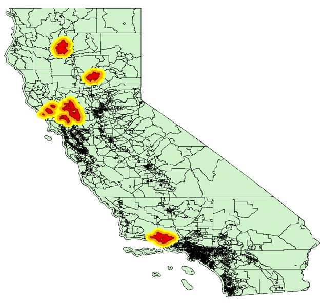
group).9 Figure 1 shows the geographic location of the five extreme wildfires in California between 2016 and 2020, and
the 1-, 5-, and 10-mile peripheral rings. In Figure 2 we zoom in on the Camp Fire, to better explore the fire footprint
and peripheral rings at the census block level. Our sample design allows us to difference away smoke incidence and
thus identify fire effects (see additional discussion below). Results of the fire analyses show a significant increase
in net migration from tracts that experienced the most destructive wildfires as well as a marked decrease in house
prices in the quarters immediately following the fire event. We also find a near-term increase in mortgage, credit card,
and personal loan delinquency among consumers in the fire zone, with a more pronounced effect for the much larger
Camp Fire than for the three other extreme wildfires. Adverse household fire zone treatment effects typically persisted
multiple quarters after the fire.
To better understand the delinquency results, we use individual account-level data from the Y-14M to study credit
card spending, repayment, and monthly balance. Interestingly, we find that post-fire, treated households in the fire
zone on average increased spending but paid down credit card debt even more, resulting in a decline in monthly
balance. While the combination of reduced credit card indebtedness (repayment in excess of spending) and increased
delinquency seem puzzling, further analysis showed that the reduction of credit card balance occurred largely among
homeowners, whereas increased credit card delinquencies were evidenced among the renter population, especially
those with lower credit scores.
Fire damage typically is covered by homeowner’s insurance. In recent years, in areas of increased wildfire-related
insurance payout and risk, related coverage in California often has been excluded from the standard homeowner’s
insurance policy. In response, the State of California has made limited fire coverage available via the California FAIR
Plan (Biswas et al., 2023).10 Among homeowners, our estimated attenuation in adverse household financial impacts
(including paydown in credit card balances post-wildfire) likely reflects use of funds from insurance claim payout to
reduce debt, consistent with findings from the flood disaster literature (Gallagher and Hartley (2017), Billings et al.
(2022)). In contrast, renters typically receive limited fire insurance payout and may experience financial distress owing
9
For more information, see Figure 2. Our results are also robust to definition of control groups that are 1-2 miles
from the fire zone and 1-10 miles from the fire zone.
10
The California FAIR Plan provides basic insurance to satisfy the lender requirement that the home be insured
against the risk of fire. While the FAIR Plan policy covers damage from fire, smoke, lightning, and windstorms,
it does not cover other common elements of homeowners property insurance including theft, flood, earthquake, or
personal liability. The California FAIR Plan coverage is typically more expensive than private policies owing to the
high-concentration of high risk borrowers.
3
to use of their own limited resources to cope with adverse fire effect, including work disruption as well as event-related
health expenses.
    We then explore the household financial effects of wildfire-attributable smoke and particulate emissions as are
diffused broadly beyond the fire zone. We first show that extreme wildfires cause marked increases in air pollution.
Similar to Miller et al. (2021), we employ daily satellite-based measures of wildfire smoke plumes in a difference-in-
differences framework to estimate related ground-level air pollution effects as measured by PM2.5. After establishing
the causal relationship between smoke and air pollution, we proceed to estimate the impacts of fire-induced air pol-
lution on credit outcomes. Again we apply a difference-in-differences framework in a panel regression setting. In an
effort to assure that variations in ground level air pollution derive from fire-related smoke, we adopt two approaches.
First, we create a measure of fire-attributable air pollution by taking the difference between fire month ground pol-
lution PM2.5 levels and same month PM2.5 levels in the prior year. Second, we estimate the effects of particulate
emissions using an instrumental variable approach. Due to the granularity of our data, we include consumer- or credit
account-level fixed effects, so as to largely alleviate concerns of omitted variable bias.
    Our results provide new evidence of adverse causal impacts of distant wildfire-induced air pollution on credit
outcomes. We find significant increases in credit card spending as well as marked declines in credit card payments in
the wake of the smoke event. Those findings are largely evidenced among zip codes well beyond the fire zone that
experienced large spikes in wildfire-induced pollution in the quarters immediately following the wildfire event. Results
also show sizable increases in child emergency visits and asthma emergency department visits well beyond the fire zone
and in the wake of a wildfire-induced smoke event. In the five quarters following the Camp Fire, the combination of
added credit card spending and reduced credit card repayment among consumers experiencing high levels of wildfire-
induced particulate pollution resulted in an additional $500 per annum in credit card balance. Further analysis indicates
that the reduction in credit card repayment is evidenced primarily among lower credit score borrowers, consistent with
the idea that those borrowers, in the absence of adequate government assistance, typically have fewer resources to
cope with natural disasters. In contrast, the increase in credit card spending is found largely among prime borrowers.
Those borrowers likely have the capacity to spend more on preventive measures to combat air pollution induced by
the wildfire.
    As anticipated, the estimated far-flung wildfire-attributable pollution treatment effects are smaller in magnitude
than those estimated for burn zone households. For example, the Camp Fire resulted in an average 45 percent increase
in the likelihood of credit card past due among burn zone households, whereas distant wildfire-attributable emissions

                                                            4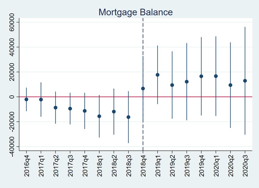
and particulate pollution are associated with a 20 percent increase in credit card past due. However, the pollution
results are highly salient, given the substantially larger geographies and populations treated by far-flung wildfire-
related emissions. As detailed below, if we conservatively impute estimated pollution effects of the Camp Fire to
the 19 million people in the New York Metro Area exposed to heavy smoke and pollution in the wake of the 2023
Canadian wildfires, a back-of-the-envelope calculation suggests that affected households incurred an incremental $3
billion in credit card spending and an added $4 billion in credit card debt.
       Three recent papers, including Issler et al. (2020), McConnell et al. (2021), and Biswas et al. (2023), examine
the effects of wildfires on burn zone housing and consumer outcomes.11 We augment those studies to estimate the
effects of extreme wildfires and wildfire-attributed air pollution on a broad array of household financial outcomes.
For example, both burn zone and broadly dispersed wildfire-induced air pollution result in increased delinquencies
in personal and retail store debt as well as higher levels of mortgage and credit card debt. We also find interesting
heterogeneity in treatment effects, whereby estimated fire effects on credit card debt and repayment differ among
homeowners and renters, likely owing in part to the provision of damage-related insurance payouts to homeowners
with damaged properties in the fire zone. The incidence of far-flung smoke and air pollution events has become
significantly more pronounced in the wake of major wildfire events in North America and Europe during the summer
of 2023. Failure to account for broadly diffused and growing consequential fire emissions effects yields only a partial
and incomplete picture of these extreme climatic events.
       The remainder of the paper is organized as follows: Section II describes the data and sample construction. Section
III discusses the framework and empirical methodology used in the paper, whereas Section IV presents the empirical
results. Section V concludes.
  11
     There are a few other papers that evaluate the effect of air pollution on housing and credit outcomes. Amini et al.
(2022) analyze the causal effect of air pollution on Iran’s housing market by exploiting increases in air pollution due to
sanctions that targeted gasoline imports and find that a 10% increase in the outdoor concentration of nitrogen dioxide
leads to a decrease in housing prices of around 0.6%–0.8%. Zheng et al. (2014) use data from China and find that
a 10% decrease in neighborhood pollution is associated with a 0.76% increase in local home prices, and Chay and
Greenstone (2003) estimate an elasticity in the range of 0.20 to 0.35. Lopez and Tzur-Ilan (2023) analyze the effect
of air pollution exposure on rent prices, using quasi-experimental exposures to wildfire smoke shocks, and find that an
increase in one unit of PM2.5 reduces the average rent by 0.7%.

                                                             5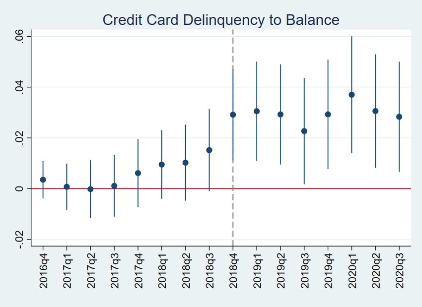
II.          Data

A.         Data on Wildfires

          We employ information on wildfire damage compiled by the U.S. Department of Homeland Security National
Incident Management System/Incident Command System (ICS). While these data have been publicly available for
many years, they have only recently been processed by St Denis et al. (2020) into an accessible format available for
broad utilization. A major benefit of the ICS data set is that it reports direct measures of hazard impact (e.g., counts
of structures destroyed or damaged), rather than the dollar value of damaged property. The latter approach, utilized
by the Spatial Hazards Events and Losses Database for the United States (SHELDUS) and the National Oceanic and
Atmospheric Administration (NOAA) National Centers for Environmental Information, fails to distinguish between
widespread fire-related structural damage and that to a small number of high-value properties. The ICS data provide
insights important to the assessment of household financial impacts of wildfire disasters (for more information, see
McConnell et al. (2021)). For purposes of this study, we linked the ICS data to the U.S. Forest Service Monitoring
Trends in Burn Severity (MTBS) database, which documents the spatial footprint of wildfire burn perimeters (Eiden-
shink et al. (2007)). For sampled wildfire events, we identify the census blocks/tracts/zip codes included in the fire
burn perimeter and beyond. We focus on extreme wildfires that damaged or destroyed more than 1,000 structures (for
a list of extreme wildfires, see Table 1). Those fires account for roughly 3 percent of all wildfires.

B.          Wildfire Smoke Data

          Miller et al. (2021) developed measures of daily smoke exposure using information on wildfire smoke from
the NOAA’s Hazard Mapping System (HMS).12 The HMS uses observations from the Geostationary Operational
Environmental Satellite, which produces imagery at a 1-km resolution for visual bands and a 2-km resolution for
infrared bands, to identify fire and smoke emissions over the contiguous United States (Ruminski et al., 2006). Smoke
analysts process the satellite data to draw geo-referenced polygons that represent the spatial diffusion of wildfire smoke
plumes detected each day. Plumes are typically drawn twice per day, once shortly before sunrise and once shortly after
sunset. We similarly employ the HMS smoke plume data from 2016 to 2020 to construct an indicator of smoke
exposure at the tract level for each day of the sample period. Our primary measure of smoke exposure is an indicator
     12
    These data come from an operational group of NOAA experts who rely on satellite imageries to identify the
location and the movements of every wildfire smoke plume in the U.S..

                                                            6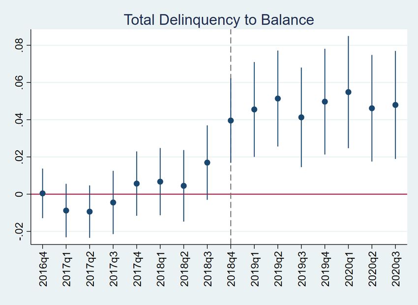
of whether a tract is fully covered by a smoke plume on a given day.

C. Pollution Data

       We obtain ambient air pollution data from the EPA’s Air Quality System. We use daily ground monitor readings
for EPA “criteria pollutants,” including a measure of particulate matter (PM2.5). To measure air pollution for a tract,
we take the distance-weighted average of two or three valid readings for each pollutant from monitors closest to a
tract’s centroid. We spatially intersect these data with census tract boundary files and link them to individual-level
administrative records.
       Figure 5 and Appendix Figures A.1 and A.2 show changes in wildfire smoke and pollution levels for the 2018
Camp Fire, Carr Fire, and Thomas Fire in California in the months prior to and following the fire. Wildfire smoke
plumes are an important source of air pollution and travel hundreds of miles downwind, allowing us to identify the
distant effects of smoke exposure separately from wildfire damage within the burn perimeter. We also use data from
Childs et al. (2022), who develop a machine learning model of daily wildfire-driven PM2.5 concentrations using a
combination of ground, satellite, and reanalysis data sources. The authors generate daily estimates of smoke PM2.5
over a 10 km-by-10 km grid across the contiguous U.S. from 2006 to 2020.13

D.       Credit, Housing, and Migration Data

       We measure household credit outcomes using the Federal Reserve Bank of New York Consumer Credit Panel/Equifax
data (CCP). The CCP is a nationally representative 5% random sample of individuals with a credit report.14 The panel
provides detailed credit-report data for (anonymous) individuals and households in quarterly increments beginning
in 1999. The data cover all major categories of household debt, including mortgages and credit cards, inclusive of
number of accounts, balances, and credit delinquencies. For more information, see Lee and van der Klaauw (2010).
The CCP also can be used to measure migration as we can trace individual consumers moving from one location (e.g.,
census tract or census block) to another using the consumer’s mailing address.
  13
      Childs et al. (2022) find that the number of people in locations with at least one day of smoke PM2.5 above 100
µg/m3 per year has increased 27-fold over the last decade, including nearly 25 million people in 2020 alone. We use
this estimation to calculate the salient effect of wildfire smoke.
   14
      The database also contains information on all persons with credit files residing in the same household as the
primary sampled individual. Household members are added to the sample based on the mailing address in the existing
credit files.

                                                          7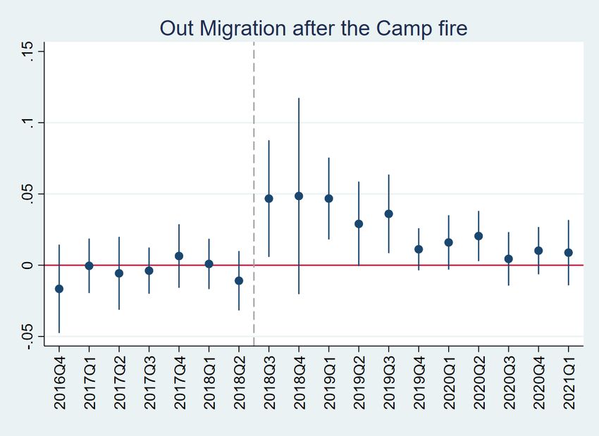
In order to contrast outcomes across housing tenure status (homeowners vs renters), we leverage another dataset,
the Credit Risk Insight Servicing McDash (CRISM) data. CRISM is an anonymous credit file match from Equifax’s
full population of consumer credit reports to the Black Knight McDash loan level mortgage dataset (as compared
to the 5 percent random sample of the CCP).15 Hence, all borrowers in CRISM are mortgage borrowers and thus
homeowners. CRISM covers about 60 percent of the U.S. mortgage market during our sample period. Another
advantage of the CRISM data is that it is updated monthly, rather than quarterly as in the CCP.
          Our primary source for housing market outcomes is the CoreLogic Home Price Index (HPI) database. The Core-
Logic HPI is quarterly in frequency and available at the census region, state, Core Based Statistical Area (CBSA),
county, and zip code levels. We use the zip code level HPI and convert it to a census tract level HPI using the zip code-
census tract crosswalk. The CoreLogic HPI is constructed using the weighted repeat sales methodology. In addition
to the price indices, the database also includes information on the number of repeated sales used to build the index for
the date period specified, and information on the median home price for repeat sales observations for the geography
and period specified. We also used information from the U.S. Department of Housing and Urban Development (HUD)
together with the United States Postal Service (USPS) on addresses identified by the USPS as having been ”Vacant”
or ”No-Stat” in the previous quarter to measure the changes in the share of vacant residential properties over time.

E.         Consumer Spending Data

          To supplement the CCP data, we obtain account-level information on consumer credit card activity from the
Federal Reserve Y-14M regulatory reports. In addition to its higher frequency, the monthly Y-14M data have an
important advantage, in that they contain detailed credit card spending, payment and balance information, tracking
the same accounts monthly. The Y-14M data also contain anonymized up-to-date information on the consumer and
the account. Such information includes borrower contemporaneous credit score, current spending limit of the credit
card account, age of the account, contemporaneous interest rate, and borrower geographic location at the 9-digit zip
code.16 The data also contain credit performance information including an account past due indicator. See Agarwal
et al. (2020) for more information. The Y14M credit card data are available from June 2013. For purposes of our
study, we use data from January 2016 to December 2019, centering around the month of each wildfire in our analysis.
     15
      CRISM is constructed with a proprietary and confidential matching process. In the matching process, Equifax
uses anonymous fields such as original and current mortgage balance, origination date, zip Code, and payment history
to match each loan in the McDash dataset to a particular consumer’s tradeline in Equifax.
   16
      Some accounts only have the 5-digit zip code.

                                                               8
F.     Summary Statistics

     Table A.2 reports summary credit information on individuals living in the wildfire zones, compared to those living
(1-5 miles) outside the fire zones, during the six quarters before and after the fire event. Summary statistics are reported
for average outcomes for the set of five sampled extreme wildfires (Camp, Carr, Thomas, Central LNU Complex, and
LNU Lightning Complex fires). The table shows that individuals residing in the fire zones were older and had a higher
Equifax Risk Score and lower mortgage balance. In terms of the number of credit accounts, individuals residing in the
fire zones had fewer credit card and personal loan accounts, but a higher number of first mortgage accounts. Further,
individuals residing in the fire zones were less likely to be delinquent on their personal loans, on average, but more
likely to be delinquent on their mortgage loans. Overall, individuals residing in the fire zones had lower bank card
balances but higher personal loan balances, on average.

III.      Research Strategy

A.     Effects of Wildfires on Migration, House Prices, and Household Financial Outcomes

     To assess the effects of extreme wildfires on migration, house price, and household financial outcomes, we estimate
panel data models in a difference-in-differences framework at the census tract and individual consumer/account-level.
Consistent with Figures 3, A.4, A.5, and A.6, we assume that trends in outcomes are similar for the treated and control
groups absent the wildfires.

A.1. Census Tract-Level Difference-in-Differences Estimates of Extreme Wildfire Impacts on Mi-
        gration and House Prices

     We compare net-migration (out-migration minus in-migration) and house price changes in wildfire “treated” tracts
(i.e., tracts within the burn area) relative to “control” tracts (e.g., tracts 1-5 miles from the fire perimeter) for the
composite sample of all five extreme wildfires. We take a “donut approach” by carving out the areas that are 0-1
miles from the fire perimeter to obviate the need to assess spillover effects of the wildfires on immediate surrounding
areas. We also present results for the Camp Fire, the largest wildfire to date in terms of structure loss (for more details,
see Table 1). We compare pre-event quarters with post-event quarters. In the case of the November 2018 Camp
Fire, we limit the analysis to eight pre-event quarters and six post-event quarters so as to avoid possible COVID-19

                                                             9
contamination commencing from the first quarter of 2020 and to allow clean assessment of fire effects on housing and
credit outcomes rather than those associated with COVID-19.
All census tract migration and house price models employ a difference-in-differences specification to estimate the
effects of wildfire structure loss on net migration and on house prices. The models take the general form:
Yc,t = β ∗ Firec,t ∗ Postc,t + τt + ζc + εc,t , (1)
where Yc,t is a measure of net-migration in census tract c in quarter t, defined as the total number of out-migrants minus
in-migrants divided by the total population at the start of a period within a tract. Firec,t represents a fire loss indicator
(1 or 0), Postc,t represents a post-fire indicator (1 or 0), and εc,t represents the error term. The interaction between
these variables is the primary term of interest, with a significant coefficient indicating that net migration or house price
changes associated with fire-affected units are significantly different in the post-fire period relative to outcomes in
neighboring control tracts. We also include two-way fixed effects, quarter fixed effects and census tract fixed effects,
to account for unobserved time-varying factors and for time-invariant characteristics of each spatial unit. As discussed
below, we undertake similar analyses of house prices. All models report heteroskedasticity consistent robust standard
errors clustered by census tract.
A.2. Consumer- and Account-Level Difference-in-Differences Estimates of Extreme Wildfire
Impacts on Household Financial Outcomes
We next employ similar models to assess the effects of extreme fire events on households’ financial outcomes. We
use consumer-level panel data from CCP and CRISM for pre- and post-event quarters to estimate the following model:
Yi,t = β ∗ Firei,t ∗ Posti,t + τt + ζi + εit , (2)
where Yi,t is the outcome measure for individual i in time t (quarterly for CCP and monthly for CRISM). The Firei,t
term is a dummy variable that takes on the value of one if the individual resides in a census block in the fire zone
and zero if the census block is outside the fire zone (1 mile and up to 5 miles). The categorical term Posti,t takes on
the value of 1 after the fire event and 0 prior to the event. τt and ζi are time- and consumer/account-fixed effects. In
this specification, we interpret the interaction term as the effect of living in a treated census block in quarter/month t
10relative to the fire quarter.
We also use the Federal Reserve’s Y-14M data to estimate a similar panel data model in a difference-in-differences
framework. As discussed above, the Y-14M data are monthly in frequency at the individual credit card account-level.
More importantly, they include detailed spending and payment information, in addition to the balance and delinquency
information available in the CCP and CRISM.
B. Effects of Wildfire Smoke and Pollution on Household Financial Outcomes
B.1. The Effect of Smoke on Air Pollution
We next turn to assessment of smoke and pollution effects. As discussed below, we use variation in wildfire
smoke and related air pollution exposure to identify the causal effects of wildfire-induced shocks to air pollution on
credit outcomes. Wildfire smoke plumes are a natural source of air pollution and travel far from the wildfire event,
allowing us to identify the effects of far flung smoke and pollution exposure as distinct from the burn zone fire effects.
The pollution emissions exposure analysis is undertaken for households living up to 30 miles from the fire perimeter.
We first present evidence of the average effect of wildfire smoke on local air quality using the following event study
specification:
20
X
PM2.5c,d = βτ ∗ S mokeDayc,d+τ + αc,day−o f −year + αc,month−year + εc,d . (3)
τ=−20
Figure A.3 shows results of an event study of the effects of smoke on air pollution among census tracts that
experienced smoke and those that did not for the 20 days before and after the Camp Fire. In the aftermath of the Camp
Fire, there was a sharp increase in pollution levels in the census tracts that experienced smoke to roughly 60 µg/m3 ,
equivalent to pollution levels measured in Beijing that same day.17
Next, we aggregate the daily smoke exposure data to the monthly level to construct our focal independent variable
and observe its effect on PM2.5 for all zip codes that are located 30 miles from the fire event. The timeframe extends
to 12 months after the fire. Using observations for each zip code z and month-year t:
PM2.5z,t = β ∗ S mokeDaysMonthz,t + τt + ζz + εz,t , (4)
17
According to the CDC, exposure to PM2.5 above 12 is considered risky and has negative health consequences.
11where S mokeDaysMonthz,t is defined as the number of smoke days in month t in zip code z. The regression equation
includes zip code and month-year fixed effects. In some specifications, we use annual fixed effects (instead of month-
year fixed effects). We also examine the effect of changes in smoke on changes in pollution, using delta smoke and
pollution terms, which are calculated as the changes in smoke days and pollution levels compared with the same month
in 2015.
B.2. Effects of Wildfire-Induced Air Pollution on Household Financial Outcomes
To estimate the effects of wildfire-induced air pollution on household financial outcomes, we again employ panel
data models in a difference-in-differences framework. To isolate the effect of broadly-diffused smoke and air pollution
from that of the wildfire itself, we focus on zip codes outside the wildfire burn area but within 30 miles from the fire
perimeter. We rank order zip codes surrounding each fire based on the level of pollution in the four weeks immediately
following the onset of the fire and then divide those zip codes into three groups: treated zip codes defined by those
in the top quartile of particulate pollution; control zip codes defined by those in the bottom quartile of particulate
pollution; and remaining zip codes which are excluded from the analysis. On the time dimension, we define the
sample to include five to eight quarters, depending on data availability, before and after each fire. We estimate the
following model:
⃗ + τt + ζi + εi,t ,
Yi,t = γ ∗ Pollutionz ∗ A f ter f irez,t + Xi,t B (5)
where Yi,t is the outcome measure for individual/account i at time t (quarterly frequency for the CCP and monthly
frequency for the CRISM and Y-14M). Pollutionz is a dummy variable that takes on the value of one if the individual
resides in zip code z that experienced pollution levels in excess of the 75th percentile within four weeks of the fire, and
zero if not. The categorical term A f ter f ire takes on the value of one after the fire event and zero prior to the event.
Xi,t are time-varying borrower characteristics such as updated borrower Equifax Risk Score. τt and ζi are time- and
consumer/account-fixed effects.
To assure that variations in ground level air pollution derive from fire-related smoke, we adopt two approaches.
Firstly, we create a measure of fire-attributable air pollution by taking the difference between fire month ground
pollution PM2.5 levels and baseline PM2.5 levels, defined as the same month PM2.5 levels in the prior three years
(excluding any days when there was wildfire-related smoke). Hence, the regression becomes:
⃗ + τt + ζi + εi,t .
Yi,t = γ ∗ ∆PM2.5z ∗ A f ter f irez,t + Xi,t B (6)
12We also estimate the effect of fire-induced air pollution on household financial outcomes using an instrumental
variable approach. One instrument is the number of smoke days experienced by a zip code in a specific month. The
first stage of this instrumental variable approach is similar to that specified in equation 4. However, here we leverage
the work of Childs et al. (2022), which provides a more sophisticated approach to first-stage estimation. Childs et al.
(2022) use a machine learning model to estimate smoke-driven pollutants for the contiguous U.S. from 2006 to 2020.
We use their estimates of smoke PM2.5 and run the second stage of our IV regression as:
Yi,t = γ ∗ PM2.5 ⃗ + τt + ζi + εi,t .
\ z ∗ A f ter f irez,t + Xi,t B (7)
\ z are the zip code-level daily estimates obtained from the Stanford University Environmental
Here the PM2.5
18
Change and Human Outcomes (ECHO) Lab aggregated to monthly frequency. In order to evaluate how wildfire-
induced air pollution dissipates over time, we also run event-study type of regressions in a similar difference-in-
differences setting.
It is noteworthy that when we estimate the fire effects, we focus on treated areas within the fire boundary and
control areas up to 5 miles from the fire perimeter. As discussed below, the entirety of the spatial footprint of the
fire study (both treatment and control areas) were treated by fire-related smoke. Hence, our difference-in-differences
approach by design differences out the smoke/pollution effects so as to allow us to identify burn zone fire effects. In
our subsequent analysis of smoke and particulate air pollution, we carve out the fire perimeter and immediate adjacent
areas. Here our sample design allows us to focus on distant smoke and pollution effects 5 to 30 miles beyond the fire
zone.
IV. Results
A. Effects of Extreme Wildfires on Net-Migration and House Prices
Table 2 presents findings of estimation of the effects of extreme wildfires on household net-migration. We compare
wildfire treated tracts (e.g., tracts within the burn footprint) to control tracts for the Camp Fire. The Camp Fire occurred
in November 2018 in Butte County, California and destroyed more than 18,000 buildings in the town of Paradise
and surrounding unincorporated areas of Magalia, Concow, and Yankee Hill. To date, that fire is the most extreme
18
https://www.stanfordecholab.com/wildfire smoke.
13of U.S. wildfire events, destroying more than twice as many structures as any other sampled extreme wildfire (See
Table 1). The first three columns in Table 2 compare the fire zone to those 1-5 miles from the Camp Fire. Overall,
findings indicate that the Camp Fire is associated with sizable and significant net out-migration among residents of
surrounding control zones. The estimated migration effects are larger among control census tracts more proximate
to the fire treatment area and decline monotonically with distance from the fire zone. Columns 4 and 5 of Table 2
compare fire zone tracts to those that are 1-10 miles from the fire (column 4) and to tracts that are 1-20 miles from the
fire (column 5). Overall, while the Camp Fire did not appear to significantly affect in-migration, findings do indicate a
significant increment to out-migration. Census tracts up to 5 miles from the perimeter of the Camp Fire experienced an
additional 18 net exits per 1,000 residents compared with fire zone tracts. The estimated effect is stable to tracts that are
10 and 20 miles from the Camp Fire. We further explore the time dynamic of estimated fire-related migration effects.
Figure A.4 shows that adverse effects of Camp Fire on out- and net-migration are substantial in the year following the
fire; subsequently, household migratory flows largely revert to pre-fire levels. The results are consistent with previous
research on the effect of the Camp Fire (Issler et al. (2020), McConnell et al. (2021)).19 Our findings also are consistent
with prior research on a smaller subset of FEMA disaster-declared wildfires (Winkler and Rouleau, 2021), and with
dynamic spatial models of the U.S. economy of adaptation to climate change (Cruz and Rossi-Hansberg (2021), Bilal
and Rossi-Hansberg (2023)).
Table 3 reports on census tract level difference-in-differences estimates of the effect of the 2018 Camp Fire on
house prices. Findings indicate that the Camp Fire caused a 17.5 percent decline in house prices in the fire zone
compared with control census tracts some six quarters subsequent to the fire event. In dollar terms, Table 3 shows
that the Camp Fire caused a decline of $34,553 (compared with a median repeat sales value of $280,007 in the treated
Camp Fire area). Table 3 also shows that the repeat sales median house price in the area treated by the Camp Fire
remained damped by roughly $10,000 throughout the post-fire study period. Column 4 in Table 3 shows a significant
increase in residential vacancy rates.
Our findings on migration response to extreme wildfire events are consistent with other papers showing similar
net exit of population in the wake of other climate-related natural disasters. Indeed, a growing literature identifies
migration as among the most consequential outcomes of and adaptive mechanisms to climate change (Black et al.,
2011). Among papers focused on the U.S., Mullins and Bharadwaj (2021) apply IRS county place-to-place data for
19
McConnell et al. (2021) similarly found that among the top 5 percent most destructive wildfires, wildfire damage
resulted in out-migration of residents.
14the period 1983-2017 and find that an additional day of mean temperature between 80 and90◦ F results in increased
annual out-migration of households by 0.43% relative to a day with a mean temperature between 60 and 70◦ F, while
a single additional day with greater than 90◦ F increases yearly outgoing migration by 0.96%. Boustan et al. (2012)
estimate the long-run U.S. migration response to natural disasters and found significant reductions to in-migration to
counties struck by floods and hurricanes. Gallagher and Hartley (2017) estimate an elevated out-migration response
and only partial subsequent return among New Orleans residents that experienced higher levels of flooding in the
wake of Hurricane Katrina. Bleemer and van der Klaauw (2019) and Deryugina et al. (2018) similarly find large and
persistent effects of Hurricane Katrina on movement of New Orleans residents from the city.
B. Effects of Extreme Wildfires on Household Financial Distress
The impact of wildfire events on household finance is unclear a priori. On the one hand, wildfires may result in
destruction of physical property and disruption of work so as to result in household financial distress. However, com-
pensation of household economic loss via wildfire or standard homeowners insurance may mitigate financial distress.
Further, governmental and philanthropic emergency assistance may help to dampen adverse financial effects. Existing
empirical evidence is mixed. For example, for mortgage performance, Issler et al. (2020) find little impact of wildfire
on household finance. Biswas et al. (2023) find some evidence of elevated mortgage delinquencies only among dam-
aged properties in fire burn areas. McConnell et al. (2021) provide evidence that consumer credit distress, including
loan delinquency, personal bankruptcy, and home foreclosure, improve rather than deteriorate in the aftermath of a
wildfire, but that the changes are not statistically significant.
To explore the effect of extreme wildfires on household financial distress, we firstly employ the FRBNY Con-
sumer Credit Panel/Equifax Data (CCP). Recall that the CCP is a 5% random sample of all U.S. individuals with a
credit file and includes consumer-level quarterly panel data containing detailed information on consumer liabilities,
delinquencies, and other characteristics. Table 4 shows the effect of the Camp Fire on consumer financial distress,
estimated in a difference-in-differences framework following equation 2. Note that our treated group is comprised of
consumers living in census blocks within the Camp Fire burn footprint, whereas the control group includes consumers
living 1-5 miles from the fire perimeter. Dependent variables in columns 1-4 include mortgage delinquency, credit
card delinquency, personal loan delinquency, and retail/store card delinquency, respectively. Columns 1-3 indicate
that the Camp Fire resulted in statistically significant increases in mortgage, consumer credit card, and personal loan
delinquencies. For example, Column 2 shows that consumers living in Camp Fire burn zone experienced an additional
152 percentage point (pp) rise in credit card delinquency following the Camp Fire, compared to consumers not directly
affected by the fire (those living 1-5 miles from the fire perimeter). This effect is economically significant given an av-
erage credit card delinquency rate of about 4 percent in our sample. All regressions include year-quarter and consumer
fixed effects.
Table 4 provides estimates of average treatment effects over the eight quarters following the Camp Fire. In
Figure 3, we plot the quarter-by-quarter treatment effects of the fire, estimated using a similar difference-in-differences
approach. Panels A-D show estimated effects on consumer total delinquency (delinquencies across all credit accounts),
mortgage delinquency, credit card delinquency, and personal loan delinquency, respectively. Findings indicate that the
estimated wildfire effects on credit card delinquency persisted over the full two year post-fire period.
To better understand the effects of wildfire on credit delinquencies, we turn next to the Federal Reserve Y-14M
credit card data. An advantage of the Y14M is that we observe not only delinquencies but also credit card spending,
repayment, and balance at the monthly account level. We follow the same difference-in-differences approach in esti-
mating wildfire effects using the account-month panel. The granularity of our data further allow us to include two-way
fixed effects. In addition, we control for time-varying account attributes such as updated borrower credit score and
current credit limit of the account.
In Table 5, we report our estimates of the effects of the Camp Fire on credit card spending, payment, balance,
and past due in columns 1-4, respectively. To account for possible seasonality, we use year-over-year changes in our
dependent variables. Changes in credit card spending, repayment, and balance, as shown in the first three columns,
are annualized dollar amounts. As shown in the table, borrowers residing in the wildfire burn area engaged in roughly
$1,100 per annum additional spending in the 14 months following the fire, relative to borrowers residing 1-5 miles
outside the burn area (column 1). Interestingly, estimates also show that fire zone residents engaged in about $1,500
per annum more in repayment, relative to those outside of the fire burn zone (column 2). As a result, households living
within the wildfire burn perimeter accumulated an estimated $1,900 per annum less in credit card debt (column 3).
Column 4 of Table 5 shows an elevated account past due among borrowers residing in the wildfire burn area, consistent
with the increased credit card delinquency result we see from the CCP analysis discussed above.
In Figure 4, we plot our estimated effects of the Camp Fire on credit card spending and repayment quarter-over-
quarter. Results show a clear increase in credit card spending and repayment immediately following the wildfire among
borrowers residing in the fire zone. The increases in spending and repayment peaked in the second quarter post-fire
and then tapered in quarters 3-5.
16The combination of reduced credit card indebtedness (repayment in excess of spending) and increased delin-
quency/past due shown in Tables 4 and 5 appear puzzling on face value. In that regard, we have two hypotheses:
Firstly, we hypothesize that homeowners whose property was damaged by the fire used payouts from insurance claims
to reduce debt inclusive of credit card balance. Secondly, households who did not receive insurance payout were likely
to become delinquent due to increased credit card spending to cope with the wildfire.
Unfortunately, the Y-14 data does not contain information on borrower tenure status. We thus return to the CCP
data and segment our sample into homeowners and renters.20 We further separate high Equifax Risk Score borrowers
from low Equifax Risk Score borrowers. We then repeat our difference-in-differences analysis using the segmented
CCP sample. Table 6 reports our results on credit card balance (Panel A) and credit card delinquency (Panel B). From
these results, we see that homeowners residing in the fire zone (and thus likely to have experienced property damage)
did pay down their credit card balance more than those in the control group (Panel A column 2). For those consumers,
we do not find any increase in credit card delinquency (Panel B columns 1 and 2). In contrast, the elevated credit card
delinquencies emanate from lower Equifax Risk Score renters (Panel B column 3).
These results and the results in the previous two tables paint a picture of interplay between fire damage and
insurance payout in shaping consumer financial outcomes. Specifically, the Camp Fire caused property damage and
work disruptions; in order to cope with the adverse wildfire effects, consumers spent more using their credit cards.
However, homeowners who received insurance claims payout had greater financial capacity to pay down their debt
inclusive of credit card balance; in contrast, renters lacking insurance payout had fewer financial resources to pay
down their elevated credit card debt and were more likely to fall into delinquency.
The insurance claims payout story is consistent with Gallagher and Hartley (2017) findings of mortgage borrowers
using flood insurance payout to pay down their mortgages. Further, it is also supported by additional analysis displayed
in Appendix Figures A.5 and A.6. In Appendix Figure A.5, we see that for borrowers who remained in the fire zone
subsequent to the Camp Fire, both number of credit card accounts and credit card balance were reduced significantly
after the fire.21 In Appendix Figure A.6, findings from CRISM data show the decline in credit card accounts and the
balance was significantly larger for mortgage borrowers residing in the fire zone.22
20
In CCP, we define consumers with a positive mortgage balance as homeowners. By doing so, we include cash
buyers/owners in the renter category, which can cause some aggregation bias in the renter analysis. Therefore, we
excluded renters living at the same address for more than three years to avoid counting consumers as renters if they
are actually homeowners with a zero mortgage balance.
21
The number of personal loan accounts and retail credit card accounts was reduced significantly after the fire.
22
Borrowers in the CRISM sample are all mortgage borrowers as CRISM is a match between McDash mortgage
17C. The Effect of Smoke on Air Pollution
Wildfires are widely recognized as major contributors to air pollution. Burke et al. (2021) estimate that wildfires
have been the source of up to 25% of PM2.5 recorded in the U.S. in recent years, and as much as 50% of PM2.5 in
some Western regions. Further, spatial patterns in ambient smoke exposure do not coincide with typical socioeco-
nomic pollution exposure gradients. Borgschulte et al. (2022) show how smoke events map to daily ground-level air
quality, using an event study that regresses PM2.5 on a series of indicators for smoke exposure. We employ a similar
approach. In Figure A.3 we show the effect of wildfire-related smoke on air pollution, using an event study of the
20 days prior to and after the Camp Fire and among census tracts that were and were not exposed to the smoke. As
evident, in the aftermath of the Camp Fire, in census tracts treated by wildfire-related smoke, pollution levels increased
sharply, to 60 µg/m3 , roughly equivalent to pollution levels measured in Beijing on that same day. Table A.5 presents
summary information on fire-related smoke and particulate air pollution (both in levels and in changes in those terms
compared with the same month in 2015) for each of the California extreme wildfires. On average, in the aftermath
of the Camp Fire, for example, findings indicate a monthly average of five smoke days with pollution levels of 12.4.
According to the CDC, exposure to PM2.5 above 12 is considered risky and associated with negative consequences.23
Concerns regarding adverse effects of wildfire-attributable smoke and particulate pollution intensified in the North
Central and Northeast U.S. in June 2023 in the wake of widespread Canadian wildfires, which adversely impacted
large geographies and millions of households.
Table A.6 shows the effect of smoke days (and changes therein) on air particulate pollution levels, controlling for
zip code and year /(or month-year) fixed effects. We assess those effects for the 12 months subsequent to the wildfires
(and separately for Camp and Thomas fires). Results of the analysis indicate a positive and significant effect in most
specifications. Column 1 in Table A.6 shows that a one standard deviation increase in the number of smoke days
(11.3) is associated with an increase in pollution of 4.3 (compared to a mean of pollution levels after the fires of 9.7).24
Column 2 shows that on average, for all five fires, a one standard deviation increase in delta smoke (the change in
smoke days in the same months relative to 2015) is associated with an increase in pollution of 2.8 (compared with
a mean of pollution levels after the fires of 1.3). We find similar effects for the Camp and Thomas fires. Column
servicing reports and consumer credit reports.
23
Burke et al. (2022) find that since 2016, wildfire smoke has reversed previous improvements in average annual
PM2.5 concentrations in two-thirds of U.S. states, eroding 23% of previous gains on average in those states and over
50% in multiple western states.
24
Borgschulte et al. (2022) find that an average smoke day increases PM2.5 by 2.2 µg/m3 on the day of exposure,
about one-third of a standard deviation in the distribution of daily particulate matter.
184 in Table A.6 shows that a one standard deviation increase in smoke days in the two years after the Camp Fire is
associated with an increase in pollution of 6.1 (compared to a mean of pollution after the Camp Fire of 12.4). Also,
column 8 in Table A.6 shows that a one standard deviation increase in smoke days in the two years after the Thomas
Fire is associated with a pollution increase of 0.5 (compared with a mean of pollution after the Thomas fire of 6.8).25
As is evident, the increment in particulate pollution attributable to extreme wildfires is sizable.
D. Effects of Air Pollution on Borrower Credit Outcomes
In this section, we explore the effect of wildfire smoke-attributable air pollution on household credit outcomes.
As discussed above, expansive geographies and large populations beyond the actual burn perimeter may be treated
by wildfire-attributable smoke and air pollution. Indeed, heavy smoke and pollution emissions from the roughly 500
active Canadian wildfires in June 2023 resulted in dangerous and unhealthy air for tens of millions of households in
the North Central and Northeast United States.
The existing literature points to some potential channels through which wildfire smoke could affect household
financial health. First, the impact could be through the health-related spending channel. Among the most widely
documented adverse effects of ambient air pollution are those associated with health, inclusive of increases in hospi-
talization rates and premature mortality among children and the elderly (Chay and Greenstone (2003), Jayachandran
(2009), Chen et al. (2013), Deryugina et al. (2019), Anderson (2020)). Approximately one-third of U.S. households
include someone with an existing respiratory health condition at risk of serious medical complications in the wake of
prolonged exposure to the fine particulate matter (PM2.5) found in smoke (McCaffrey and Olsen (2012). Therefore,
households may face elevated indebtedness due to medical or related preventative measure spending as necessary to
cope with the smoke.
Second, the wildfire-related smoke may affect household financial health via an income channel. Smoke events
may lead to work interruption (Borgschulte et al. (2022)), increased traffic accidents (Matthews (2018)), reduced
tourism and outdoor recreation (Stotts et al. (2018)),26 and more generally to a reduction in business sales (Addoum
et al. (2023)), resulting in income loss and deterioration in household financial status in the immediate aftermath of the
event. Further, existing research shows that exposure to air pollution reduces earnings. For example, Borgschulte et al.
(2022) find that a day of county wildfire smoke exposure reduces quarterly per capita earnings by $5.20, representing
25
One possible explanation for the low levels of smoke and pollution after the Thomas Fire is the relatively open
topography and proximity to the ocean of the burn perimeter.
26
See, also, “Up in Smoke: Canada’s Outdoor Summer Season,” New York Times, July 25, 2023.
19You can also read