VURCA PROJECT Cities vulnerability to future heat waves & adaptation strategies - Project methodology and results - Centre National de ...
←
→
Page content transcription
If your browser does not render page correctly, please read the page content below

VURCA PROJECT

Cities vulnerability
to future heat waves
& adaptation strategies

Vulnérabilité URbaine aux épisodes Caniculaires
et stratégies d’Adaptation

Project methodology and results

ANR Funding
N° ANR-08-VULN-013/VURCA

                                      1
Consortium:
CIRED         (1)   Centre International de Recherche sur l’Environnement et le
                    Développement
CNRS GAME     (2)   Groupe d’études de l’Atmosphère MEtéorologique
CSTB          (3)   Université Paris-Est, Centre Scientifique et Technique du Bâtiment

Authors:
Stéphane    Hallegatte1, Vincent Viguié1, Valéry Masson2, Aude Lemonsu2,
Grégoire Pigeon , Anne-Lise Beaulant , Bruno Bueno , Colette Marchadier2,
                 2                    2             2

Jean-Luc Salagnac3.

                                    May 22, 2013
                             vurca_final_report_1_1.doc

                                           2
Summary

SYNTHESIS                                                          6
   Project identification                                          6
   Summary and key insights                                        7

SCIENTIFIC REPORT                                                 11
   INTRODUCTION                                                   11
 CHAPTER 1 Urban climate and urban economic models                12
   1.1    NEDUM Socioeconomic urban expansion model               12
   1.2    TEB SURFEX Urban climate model                          14
   1.3    How to link urban expansion and climate models?         17
 CHAPTER 2 Heat waves events in future climate                    19
   2.1    Heat waves definition                                   19
   2.2    Heat waves extraction from climate projection           20
   2.3    Heat waves classes definition                           22
   2.4    Heat waves modeling methodology                         23
 CHAPTER 3 Definition of indicators related to urban heat waves   25
   3.1    VURCA’s indicators                                      26
   3.2    Evaluation of thermal comfort                           27
   3.3    Evaluation of energy consumption                        28
   3.4    Evaluation of water consumption                         29
 CHAPTER 4 City adaptation strategies                             30
   4.1    Urban structure adaptation strategies                   30
   4.2    Building adaptation measures                            33
   4.3    Air conditioning usage adaptation measures              35
   4.4    Combined adaptation strategies                          36
 CHAPTER 5 Evaluation of adaptation strategies                    38
   5.1    Analysis of heat waves impact on present day Paris      38
   5.2    City vulnerability Vs adaptation strategies             43
 CHAPTER 6 Conclusions                                            51
   6.1    Limits of the project, and future research              51
   6.2    Interpretation and key insights                         52

REFERENCES                                                        55
   Project deliverables                                           55
   Bibliographic references                                       55

                                            3
Figures

Figure 2 - Description of NEDUM-2D model. ....................................................... 12
Figure 3 - TEB scheme ................................................................................ 14
Figure 4 - Left: Initial version of TEB without interaction between built-up covers and
    vegetation; Right: New version of TEB including vegetation inside the streets. ........ 14
Figure 5 - Diagram of the new version of TEB including the Building Energy Model. ........ 15
Figure 6 - Representation of the 3 environments considered to evaluate UTCI in TEB ...... 16
Figure 7 – Example of surface fields defined according to NEDUM’s outputs for the sprawl
    city scenario: fraction of impervious covers (left) and of private garden(right)........ 17
Figure 8 – Description of the methodology applied to translate the results of the NEDUM
    urban expansion model in input parameters for the SURFEX model. ..................... 18
Figure 9 - Methodology of HW extraction. Example for TIx..................................... 19
Figure 10 – Number of HWs (top) and of cumulated HW days (bottom) calculated by year
    over the control period (1960-1989) and both future periods (2020-2049 and 2070-
    2099) for the 9 climatic projections from ENSEMBLES. ..................................... 21
Figure 11 - Number of HWs (top) and cumulated HW days (bottom) calculated by year over
    the control period (1960-1989) and both future periods (2020-2049 and 2070-2099) for
    the 3 climatic projections of ARPEGE following 3 different emission scenarios. ....... 22
Figure 12: HW proposed classes ..................................................................... 22
Figure 13– Distribution of future HWs (over 2070-2099) by class of intensity................. 23
Figure 14 - Description of the modeling methodology ........................................... 23
Figure 15 – Example of daytime evolution of air temperature for 2003 HW (referred to as
    REF) and the four classes of HWs .............................................................. 24
Figure 16 - Representation of vulnerability ........................................................ 25
Figure 17 - Risk framework in VURCA project. .................................................... 26
Figure 18– Matrix of occurrence probabilities for future HWs (computed for the period
    2070-2099) depending on their durations and intensities. ................................. 27
Figure 19 - UTCI assessment scale in terms of thermal stress .................................. 27
Figure 20 – Daily profiles of activity (and associated UTCI) for the 5 typologies of people. 28
Figure 21 – Comparison between evaporation from gardens simulated for the scenarios with
    (blue) and without (green) watering. ......................................................... 29
Figure 22- VURCA’s adaptation strategies ......................................................... 30
Figure 23 - Comparison of rents level in the center of Paris in the three scenarios ........ 32
Figure 24 - Average distance traveled by car per household and total transport-related GHG
    emissions in the three scenarios. .............................................................. 32
Figure 25 - Total urbanized area, and total garden surface in the three scenarios ......... 33
Figure 26 – Construction periods in the past ....................................................... 33

                                                    4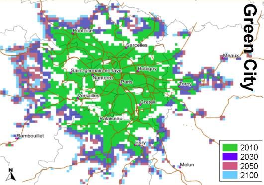
Figure 27 – Regulations and improvements steps in the future ................................. 33
Figure 28 – Overview of building adaptation measures versus building type and scenarios 35
Figure 29 - Distribution of the hours of the day according to the heat-stress thresholds of
    UTCI. The results are presented by class of intensity and by typology of people. ..... 38
Figure 30 – Number of hours spent in high heat-stress condition, cumulated day-by-day and
    expressed for an averaged day. The diagram represents HW duration on the X-axis and
    HW intensity on the Y-axis ...................................................................... 40
Figure 31 – Day-by-day evolution of cumulated energy (top, left), cumulated energy per m2
    of floor (top, right), maximum over-power (bottom, left), and over-power (i.e.
    variation in maximum power generated by an 1°C increase in air temperature:
    bottom, right) for 2006 NEDUM-Paris according to the four classes of intensity. ...... 41
Figure 32 – Daily energy consumption compared to the CLIM2 value. ........................ 42
Figure 33 – Mean daily 2-m air temperature averaged for grid points with air-conditioning
    i.e. offices only (left) and difference between 2-m air temperatures of heat waves
    from different classes of intensity (right). ................................................... 42
Figure 34 – Impacts of scenarios on both energy saving (X-axis) and gain in outdoor comfort
    (Y-axis) compared to the reference scenario for the case “Air-conditioning for all”. . 46
Figure 35 – Same than Figure 34 for 3 action levers (left) but with an additional case: the
    pie chart with colours blue/green/purple refers to the scenario combining "Green city"
    + "Watering" + "Virtuous building" but with an intensive use of AC. ...................... 47

                                                  Tables

Table 1 – Definition of all indicators used in the methodology of HW detection ............. 20
Table 2 – Description of the 25 integrated scenarios ............................................ 37
Table 3 – Description of the scenarios analyzed for the case “Air-conditioning for all”. They
    are classified according to the number of implemented action levers. .................. 44
Table 4 – Contributions of the different action levers (analyzed separately) in terms of
    energy saving, and gain in indoor and outdoor comfort. ................................... 48
Table 5 - Description of the scenarios analyzed for the case “Alternative to air-
    conditioning”. They are classified according to the number of implemented action
    levers............................................................................................... 49

                                                      5
SYNTHESIS

Project identification

Acronym       VURCA

Name          Vulnérabilité URbaine aux épisodes Caniculaires et stratégies d’Adaptation
              Urban structure vulnerability to heat waves and adaptation strategies

Funding       ANR – French National Research Agency

Coordinator   Stéphane Hallegatte – Vincent Viguié
              CIRED – 45 bis Avenue de la Belle Gabrielle
              94 736 NOGENT SUR MARNE
              stephane@hallegatte.eu ; viguie@centre-cired.fr

Consortium    CIRED           (1) Centre International de Recherche sur l’Environnement
                                  et le Développement
              CNRS GAME       (2) Groupe d’études de l’Atmosphère MEtéorologique
              CSTB            (3) Centre Scientifique et Technique du Bâtiment

Duration      4 years

Start date    January 2009

Team          Stéphane Hallegatte1, Vincent Viguié1,
Members
              Valéry Masson2, Aude Lemonsu2, Grégoire Pigeon2, Anne-Lise Beaulant2,
              Bruno Bueno2, Colette Marchadier2

              Jean-Luc Salagnac3.

                                             6
Summary and key insights
Because more than half of the world population lives there, and because most of the
economic activity takes place within them, cities appear of particular importance when
looking at the potential impacts of climate change.
Climate change can threaten cities through many different ways. One of them is the
increased risk of summer heat waves, which can be dangerous for human health and
impact energy consumption. Such a risk is reflected in climate models simulations, for all
emission scenarios, by both an increase in average summer temperatures and in
temperature variability from one year to another. Cities are particularly vulnerable to heat
waves because of the urban heat island effect, which magnifies the high temperatures in
urbanized areas.
The impact will depend on the infrastructure in place, planning policies, types of homes
and lifestyles. Several policies can be undertaken to mitigate this risk: the development of
air conditioning is one of them, and may enable to greatly decrease the health burden of
heat waves; the promotion of better building insulation or land-use policies promoting
green spaces may also be means to attenuate the negative effects of the urban heat
island.
VURCA project studies cities vulnerability to future heat wave events. Through an
interdisciplinary team consisting of climatologists, atmospheric physicists, economists and
specialists in construction, it was able to develop a framework to analyze prospective
effects of different policies aiming at reducing heat waves impacts. This project takes
Paris urban area as a case study.
Based on a demographic scenario and a scenario of transport prices evolution, Nedum-2D,
a simulation model of urban expansion developed in CIRED, was used to develop scenarios
of prospective urban expansion, distribution of the population, and average level of rents
in the city.
These scenarios were then used by TEB-SURFEX model, developed at CNRM-GAME, to
simulate, for different heat waves computed by climate models, the effect of urban heat
island. This enabled to compute energy consumption related to air conditioning use, and
the temperatures inside buildings and in the streets.
A number of results are available from this work, answering three main questions:

   1. To what extent will Paris be vulnerable to heat waves?
Paris can be strongly affected by heat waves. We computed that, without air conditioning,
at the end of the century, almost 11 heat wave days per year in average should be
expected to be spent in Paris urban area. During these days, in residential buildings, if no
AC is used, almost 7 hours and a half would be in average spent in high heat stress
conditions, i.e. with an apparent air temperature (UTCI) greater than 32°C. This could
lead to serious health consequences. In the streets, even in shadow, this duration is
higher, and almost 15 hours have to be spent in these conditions.
Urban expansion, through an increased heat island effect, could worsen heat waves
impacts. We computed that, in the scenario of high city densification (the “compact city
scenario”), in the streets, 20 minutes in high heat stress conditions should be added.

                                              7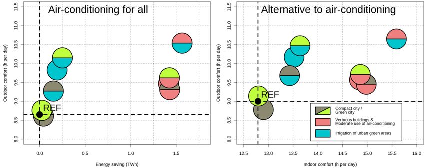
2. What would be the effect of a massive development of air-conditioning?
If a massive development of air conditioning happens happens to create more conformable
indoor ambiance and to prevent health issues, about 1.1 TWh per year of extra final
energy consumption should be expected, if a 23° temperature is to be maintained in all
residential and office buildings.
Heat released by AC systems causes a degradation of external thermal comfort, and the
duration spent under high heat stress conditions in the streets is increased by about 20
minutes.
These results were computed with the hypothesis that existing urban green spaces are
adequately watered, and this plays an important role in reducing Paris sensitivity to heat
waves. In case of water shortage, (which is almost equivalent to an urban green spaces
removal), we simulated that energy consumption would be increased by about 8%, and
that almost one hour of outdoor thermal discomfort would be added.
3. Could alternative adaptation policies enable to reduce energy demand for
air conditioning and thermal discomfort?
Energy demand for air conditioning could be an important burden in a context of
greenhouse gases reduction efforts, but adaptation policies could be implemented to
reduce this demand. We computed that:
a massive creation of parks and green spaces in Paris urban area (devoting 10% of
land surface to new parks),
stricter building insulation rules and the use of reflective materials for walls and
roofs,
and effective recommendations or policies leading to air conditioning used to
maintain 28°C in residential buildings and 26°C in offices instead of 23°C,
could together enable to reduce energy consumption by 0.7 TWh, i.e. reduce energy
consumption for AC by more than 50%. This would also reduce outdoor thermal
discomfort time by about 1 hour.
However, these policies could not a priori totally replace AC use, as 6 hours per day
would still have to be spent in high heat stress conditions in residential buildings if no
AC is to be used at all.
In conclusion, several alternative options to air-conditioning are able to significantly
reduce the vulnerability of the city in terms of both indoor and outdoor comfort.
Nevertheless, at best, a third of the day is spent under conditions of strong heat stress
inside buildings without air-conditioning.
Adaptation policies efficiency depends on the heat wave characteristics
Various adaptation policies have efficiencies which vary according to the type of heat
wave. For instance, cities sensitivity to heat waves varies greatly with the duration of the
event. Continuously high temperatures are required during a few days before indoor
temperatures reach their maximum equilibrium value. This duration was found to be about
5 days in Paris. Building insulation enables to increase this duration and therefore to be
less sensitive to short heat waves.
8
Adaptation policies implementation issues
Implementing these policies is however not an easy task. Beside the operational
difficulty to limit the use of air conditioning, the reinforcement of building insulation
would be expensive, and green spaces creation would have a high cost in terms of land use
(by decreasing residential land supply, it could increase all rents and real estate prices by
2 %, when compared to reference scenario). Green spaces creation would also reduce the
city density and could lead to increased urbanized surface, and to increased transport-
related greenhouse gases emissions (+10%). They would finally require a huge amount of
water to be efficient. If water availability stops, green spaces are found to have almost no
effect.
Among the three policies we have studied, the change in AC use (increasing temperature
set points) is the policy which has the greatest impact when considered alone. This policy,
moreover, has none of the costs or collateral effects that the two other adaptation policies
have. However, it is rather unclear how such a policy could be implemented in practice.

                                              9
A. Reference scenario: urban heat island effect is clearly        B. With the three adaptation policies: this simulation was done
visible, with a 6 °C temperature difference between the center    with the exact same conditions as map A, except that the three
of Paris and the countryside.                                     adaptation policies are supposed to have been implemented.

                                                                           Figure 1: example of simulation maps for Paris in 2100.
                                                                           Maps represent air temperature at 4 a.m. in the streets,
                                                                           after 9 days of a heat wave similar to the 2003 heat wave.
                                                                           These temperature maps were computed for a projection of
                                                                           what Paris could be in 2100, with and without the
                                                                           implementation of the three specific adaptation policies

                                                 10              C. Difference between both simulations: this map shows the
                                                                 difference between maps A and B. Air temperature decrease can
                                                                 be up to 5°C thanks to adaptation policies.
SCIENTIFIC REPORT
INTRODUCTION
Because more than half of the world population lives there, and because most of the
economic activity takes place within them, cities appear of particular importance when
looking at the potential impacts of climate change. (C. Rosenzweig et al. 2010; Hallegatte
et Corfee-Morlot 2010)
Climate change can threaten cities through many different ways. One of them is the
increased risk of summer heat waves, which can be dangerous for human health and
impact energy consumption. Such a risk is reflected in climate models simulations, for all
emission scenarios, by both an increase in average summer temperatures and in
temperature variability from one year to another. Cities are particularly vulnerable to heat
waves because of the urban heat island effect, which magnifies the high temperatures in
urbanized areas. (IPCC 2007a; Cynthia Rosenzweig et al. 2011)
The impact will depend on the infrastructure in place, planning policies, types of homes
and lifestyles (Riberon et al. 2006). Several policies can be undertaken to mitigate this
risk: the development of air conditioning is one of them, and may enable to greatly
decrease the health burden of heat waves; the promotion of better building insulation or
land-use policies promoting green spaces may also be means to attenuate the negative
effects of the urban heat island.
However, an air conditioning policy may lead to a great increase in energy consumption,
and, hence, in greenhouse gases emissions, conflicting with climate change mitigation
efforts (McEvoy, Lindley, et Handley 2006; Salagnac 2007; Hamin et Gurran 2009) ; building
energy performance improvement or green spaces policies direct costs, benefits and side
effects (e.g. the modification of urban landscape) are difficult to assess, in part because it
requires a broad interdisciplinary approach.
In this project, we aim at dealing with this issue. Through an interdisciplinary team of
researchers combining atmospheric physicists, urban economists and construction
specialists, we have developed a quantitative prospective framework that enables to
assess many different aspects of these policies, using Paris urban area as a case study.
In the first section of this report, we present the urban expansion model and the urban
climate model that we have linked and used together to do this study. In the second
section, we focus on the description of the future heat waves used in the analysis. In the
third section, we explain how we measured the future vulnerability to heat waves. We
present in the fourth section various adaptation policies, and finally in the last section how
these policies can mitigate heat wave consequences, and what are the associated direct or
indirect costs.
11CHAPTER 1
Urban climate and urban economic models
The systemic approach within VURCA project has been developed through a core of models
into a unique investigation framework: a socioeconomic urban expansion model, and an
urban climate model. A major effort has been made to:
improve of our models: see sections 1.1 and 1.2
prepare their integration: see section 1.3
1.1 NEDUM Socioeconomic urban expansion model
Urban structure and its evolution is a crucial determinant of cities vulnerability to heat
waves, through. NEDUM-2D has been developed in this project to model how the
inhabitants choose to locate in a city, how policies can influence their choice, and what
are the socio-economic effects associated to these policies.
This has been designed to create long-term scenarios for city expansion, based on
scenarios describing future land-use and transport policies in the city, on demographic
scenarios on the future total population, and on global “techno-economic” scenarios on
future income, construction cost and transport cost evolution. These techno-economic
scenarios can be produced through global general equilibrium prospective models, such as
Imaclim-R developed in CIRED (Rozenberg et al. 2010), or Markal/TIMES developed by IEA
ETSAP1. NEDUM-2D can therefore be seen as a tool to downscale at city scale global
scenarios produced by such models.
Land-use constraints
+
Transport times and costs Rents, population density,
+ floor-area ratio, and
average dwelling size
Total population
Construction costs
Average households
income
Figure 2 - Description of NEDUM-2D model.
1
http://www.iea-etsap.org/web/tools.asp
12More precisely, NEDUM-2D simulates the spatial distribution of land and real estate values,
dwelling sizes, population density, building height and density, and their evolution over
time (Figure 2). (Gusdorf et Hallegatte 2007; Viguié et Hallegatte 2012; Viguié, Hallegatte
et Rozenberg 2011) It is a dynamic model which relies on the classical urban economics
framework (Fujita 1989), but is able to capture the dynamics of urban systems, and the
importance of inertia. To produce scenarios going until the end of the century, it uses only
general and fundamental economic principles, which are likely to remain constant over the
long term. A more detailed description of the model is available in the technical report
(see Project deliverables).
Three main mechanisms drive the model. First, we suppose that households choose their
accommodation location and size by making a trade-off between the time and money they
spend for transport (i.e. to commute to their jobs) and the real estate price level (or,
equivalently, between the proximity to the city center and the housing surface they can
afford).
Second, real estate developers choose to build more or less housing (i.e. larger or smaller
building) at a specific location, depending on the local level of real estate prices. When
these prices are low, developers tend to build low density buildings, and when these prices
are high, they tend to build high density buildings.
Third, we suppose that various city characteristics do not change and adjust at the same
speed. For instance, rents can change very quickly, whereas buildings characteritsics
evolve over a much longer timescale. Building depreciation is also very slow, leading to
path dependency and lock-ins in city evolution.
Using these mechanisms, it is possible to determine the structure of the city from
information on population size, households’ income, transport network location, building
construction costs and developers behavior parameters.
In this project, this model has been first calibrated on Paris urban area (Viguié et
Hallegatte 2012). A validation of the model over the 1900–2010 period shows that the
model reproduces the available data on the city’s evolution fairly faithfully, suggesting
that the model captures the main determinants of city shape evolution. It also well
reproduces the spatial distribution of dwelling size, population density, and rents in the
urban area (Viguié, Hallegatte, et Rozenberg 2011; Viguié 2012, see also Project
deliverables)
A great part of the development of NEDUM-2D model was performed thanks to
outcome
VURCA project. An important part of the work was devoted to calibration and
VURCA’s
validation of the model on Paris urban area.2
The development of a methodology for long-term scenarios building for cities,
and for the assessment of adaptation policies over the long-term was also
developed thanks to the project.3
2
Deliverable 2.1: “Technical report on economic-urban model development”.
3
Deliverable 4.1: “Report on the long-scenario for cities, including the adaptation strategies and their economic side-
effects”.
131.2 TEB SURFEX Urban climate model
Urban climate modeling has been a research topic studied at Météo France/GAME for about
ten years. A specific urban canopy model was developed, the Town Energy Balance (TEB,
Masson 2000), in order to parameterize radiative, energetic, hydrologic, and turbulent
processes at the interface between built-up surfaces and atmosphere.
TEB is included in the surface numerical module SURFEX, and is based on a simplified
geometry description of urban covers. Built areas are represented as mean urban canyons
composed of 1 flat roof, 1 road, and 2 identical walls with isotropic street orientations
(Figure 3).
Radiation and energy balances are
resolved independently for each of these
urban facets and then aggregated for
the whole urban canyon. Mean
geometric parameters describe the
urban arrangement. The radiative and
thermal properties of materials are
associated with each urban facet.
In the VURCA project, several
improvements have been made in order
to model in a more realistic way some
aspects of urban microclimate, so that
the model is able to evaluate and
compare different adaptation strategies
linked with urban planning. Figure 3 - TEB scheme
Urban green space in TEB
The original version of TEB is only applied to built-up covers. To model the microclimate
for urban environments that include some urban green spaces, TEB is coupled with the
ISBA vegetation model but without direct micro-scale interactions between built-up and
natural covers (Figure 4, left): each model calculates the surface fluxes over the cover
types it deals with, and then these fluxes are aggregated according to the respective cover
fractions.
Figure 4 - Left: Initial version of TEB without interaction between built-up covers and vegetation;
Right: New version of TEB including vegetation inside the streets.
TEB has been improved in order to integrate explicitly the low vegetation (gardens)
between buildings (Figure 4, right) so that the geometric parameters of the urban canyon
are more realistic (especially, the canyon is wider). The radiation calculations are
14modified to account for the shadow effects of buildings on vegetation, and the
contributions of vegetation in the short and longwave radiation budget. The turbulent
fluxes over vegetation are still computed with ISBA but inside the TEB’s code by providing
ISBA the right atmospheric conditions inside the canyon. Finally, these microclimatic
variables (temperature, humidity, wind) are recomputed by including the contributions of
gardens.
Both versions of TEB have been confronted to experimental data issued from a field
campaign conducted in Israel (Lemonsu et al. 2012). A significant improvement in the
modeling of surface temperature and street-level air temperature has been highlighted. In
conclusion, this new version is better suited to study greening strategies.
Air conditioning in TEB
While the original version of TEB considered the need for heating inside the buildings and
proposed estimates of the associated energy demand (Pigeon et al. 2008), it did not take
into account the need for air-cooling. For this project focused on heat waves, it has been
essential to develop its calculation inside TEB to evaluate:
Energy demand associated to air conditioning for the different scenarios of urban
expansion and adaptation measures for buildings proposed;
Environmental impact of a massive air conditioning strategy in order to mitigate
the indoor heat stress. Indeed, according to De Munck et al. (2012), the heat
releases associated to massive air conditioning over Paris increase up to 2 °C the
urban heat island, and the associated outdoor discomfort.
During the VURCA project and in association with the MUSCADE4 project, a building energy
model (BEM) has been developed inside TEB (Figure 5). This model (TEB-BEM) uses the
same homogenous urban morphology as the original TEB but now resolves an indoor
building energy balance for a unique thermal zone with a single thermal mass that
represents the thermal inertia of construction materials inside a building (e.g. partition
walls and floors). It is based on the following processes:
Solar heat gain through the glazing for
a uniform glazing ratio over the
façade,
Heat gain through specific use of
energy inside the building,
Heat exchanges by infiltration and
ventilation with outdoor air,
Air cooling or heating according to
user specified temperature set points.
The accuracy of the model has been
evaluated against energy consumption data
collected for Toulouse during the Capitoul
field campaign leaded by the GAME (Bueno et
al. 2012). Figure 5 - Diagram of the new version of TEB
including the Building Energy Model.
4
MUSCADE is a research project, funded by ANR (reference ANR-09-VLL-003) : Modélisation Urbaine et Stratégies
d’adaptation au Changement climatique pour Anticiper la Demande et la production Energétique
15Thermal comfort model in TEB
Human body thermal comfort is not only related to air temperature but also to other local
meteorological variables (radiation, moisture, wind) and to the activity level of people.
Among the huge number of existing procedures for evaluating thermal comfort, we chose
the Universal Thermal Climate Index (UTCI, www.utci.org). This index has been
developed by the COST Action 730 for public weather service, public health system,
precautionary planning, climate impact research in the health sector, and should become
an international standard.
UTCI follows the concept of an equivalent temperature of a reference environment that
would generate the same heat stress than the actual environment. The reference
environment is defined with 50% relative humidity, with still air and a radiant temperature
equaling the air temperature. The heat stress is evaluated from the multi-node Fiala
thermoregulation model (Fiala et al. 2012) and for a person walking at 4km/h with a
metabolic rate of 135 Wm-2. Since the response of the model is multidimensional (body
core temperature, sweat rate, skin wettedness, etc...) a single dimensional index is
calculated by principal component analysis. Then, to be applied to numerical weather
predictions without running a thermoregulation model, a polynomial regression equation
(6th order, available as a software source code on www.utci.org) has been developed with
less than 1°C of error with the exact solution of the model (Bröde et al. 2012).
a. Outside, b. Outside, c. Inside building
sun-exposed people people in the shade
Figure 6 - Representation of the 3 environments considered to evaluate UTCI in TEB
This equation has been implemented in TEB, and three possible environments are
considered in order to evaluate outdoor and indoor comfort: people outside exposed to the
sun, people outside in the shade and people inside buildings (Figure 6). For each
environment, the meteorological variables to compute UTCI are adapted and especially the
radiant temperature.
A considerable work of TEB model development and evaluation against
outcome
VURCA’s
experimental data was performed for implementing:
1. Urban green spaces 5
2. Energy budget of buildings and air-conditioning systems6
3. Indoor and outdoor thermal comfort indicator for human body 7
5
Deliverable 1.1: Inclusion of vegetation in the TEB urban canopy model for improving urban microclimate modeling in
residential areas. Aude Lemonsu.
6
Deliverable 4.2 : Analyse préliminaire de l’impact de scénario du bâtiment. Grégoire Pigeon
161.3 How to link urban expansion and climate models?
NEDUM-2D model simulates the urban expansion and provides projections of the evolution
of various city characteristics, such as dwelling sizes, population density, building height
and building density (see description in Section 1.1). These outputs must be used to feed
the SURFEX land surface modelling system, but SURFEX also requieres some other
data(Figure 8):, in particular in order to describe the morphology of urban covers
Building height
Building density
Fraction of roads
Fraction of gardens
Wall density (surface of walls vs ground-based surface)
Some NEDUM-2D outputs can be provided directly to TEB but most of them must be
translated into meaningful data for TEB (SURFEX). Simple rules are then applied to deduce
the fractions of buildings, roads, and private gardens required by TEB starting from the
surface area actually devoted to residential space (excluding gardens, lobbies, etc.)
divided by the constructible surface area (referred to as Shab / Sbuild) simulated by NEDUM-
2D. These rules are based on the analysis of accurate data available for Paris intra muros
(source: Agence Parisienne d’Urbanisme (APUR) ), which indicate that buildings cover 62%
of the Parisian urban areas (excluding parks); the remaining 38% are assumed to be
covered by roads and courtyards in Paris center and by roads and private gardens in the
suburbs (Figure 7). The buildings are 18 m high in average in the city center, and 6 m high
in the suburbs.
Figure 7 – Example of surface fields defined according to NEDUM’s outputs for the sprawl city
scenario: fraction of impervious covers (left) and of private garden(right).
NEDUM-2D allows only defining the parameters related to land use and morphology in
urban areas. For natural areas (forests, crops, rivers), the project relied on the Corine
Land Cover classification.8 This classification is used in order to define the fractions of land
use and land cover outside the city for the SURFEX simulation; the descriptive and
physiological parameters of vegetation are prescribed based on the ECOCLIMAP database
(Masson et al. 2003) that associates look-up tables to the Corine Land Cover classes. No
7
Deliverable 1.2: Computation of a thermal comfort index in the TEB urban canopy model. Grégoire Pigeon.
8
http://www.eea.europa.eu/publications/COR0-landcover
17specific information is available for private gardens. They are assumed to be composed of
a fraction of grass and a fraction of trees. Their characteristics are prescribed using
homogeneous properties all over the domain coming from literature.
Finally, the TEB model needs some information on the material properties and
characteristics of buildings and air conditioning systems. These parameters are directly
defined through look-up tables that refer to the types and ages of buildings. According to
theses criteria, all buildings of the area are classified according to four different
typologies:
1. Haussmanniens buildings dating from end of 19th century
2. Multi-family housings
3. Single-family housings
4. Offices
Figure 8 – Description of the methodology applied to translate the results of the NEDUM urban
expansion model in input parameters for the SURFEX model.
A methodology has been developed in order to produce in a semi-automatic way
outcome
VURCA’s
the surface fields required for the SURFEX simulations for any integrated city
scenario9, starting from data provided by the NEDUM-2D urban expansion model
(plus complementary information linked to typology of buildings).
This systemic approach and framework then allows investigating the complex
problem of city vulnerability to heat waves by coupling tools and disciplines.
9
Deliverable 3.2 : Préparation des champs de surface pour les simulations SURFEX. Aude Lemonsu.
18CHAPTER 2
Heat waves events in future climate
As the objective is to study the city vulnerability to future heat waves, a set of climate
model projections is analyzed in order to define occurrence probability of future heat
waves over the region. A definition for heat wave events is first set, and a methodology is
then proposed to extract such events from temperature time series. The same
methodology is finally applied to a large number of climate model projections to provide a
statistical distribution of heat waves at the end of the century.
2.1 Heat waves definition
Different methodological approaches exist to determine, from observed or simulated
temperature time-series, the existence of a heat wave (HW) event (characterized by a
peak of intensity and a duration): there is no universal definition in the literature. For the
present study, a new heat wave definition is proposed in agreement with recommendations
of Robinson (2001). It combines different approaches based on climatic studies and the
definition used in French operational heat wave warning system (Plan National Canicule,
PNC):
It fits with the constraints imposed by the analysis of climatic projections (only some
meteorological variables are available and with a limited temporal resolution) by
using daily minimum and maximum temperatures (Tn and Tx, see Table 1).
It integrates in a simple way information on sanitary impacts: it computes minimum
and maximum temperature indicators (TIn and Tix, see Table 1) as moving averages
of minimum (Tn) and maximum (Tx) daily temperatures, respectively, over three
consecutive days (D, D+1, D+2). These indicators allow taking into account the heat-
stress cumulative effect over time during a heat wave.
The peak of a heat wave event is first
identified when either TIn or TIx
exceed their respective temperature
thresholds (TI1, see Figure 9) applied
by the PNC for the corresponding
country, i.e., 18 and 34°C for TIn and
TIx, in this project (Figure 9).
The heat wave duration is then
determined by all adjacent days to the
peak for which TIn and TIx values are
not, during more than two consecutive
days, smaller than the first
temperature threshold minus 2°C Figure 9 - Methodology of HW extraction.
(TI2=TI1-2, see Table 1). A minimum Example for TIx.
duration of three days is however
imposed.
19This methodology is evaluated via the extraction of observed heat waves from historical
time-series of temperature recorded at Chartres and Montereau from 1950 to 2009. The
majority of past heat waves listed in the Meteo Fance database (at the country scale) are
correctly extracted. Estimated durations are also satisfactory. The main differences are
obtained for heat waves that have mainly affected the south of France, and are
consequently not extracted or shorter.
Indicator Definition
Daily minimum (Tn) and maximum (Tx) air temperatures provided by observed time-
Tn
series issued from operational meteorological stations or by simulated time-series
Tx issued from climate model projections
TIn Moving average over three consecutive days (D, D+1, D+2) of daily minimum (TIn) and
TIx maximum (TIx) temperature
TIavg Daily average temperature indicator (calculated as the average between TIn and TIx)
Threshold of heat wave detection for the daily minimum temperature indicator time-
TIn1 series
TIn1 = 18°C for Paris region (according to PNC standards)
Threshold of heat wave detection for the daily maximum temperature indicator time-
TIx1 series
TIx1 = 34°C for Paris region (according to PNC standards)
Additional threshold defined in VURCA in order to detect a heat wave from the daily
TIavg1 average temperature indicator
TIavg1 = 26°C for Paris region (calculated as the average of TIn1 and TIx1)
Second threshold used to define the heat wave duration for the daily minimum
TIn2 temperature indicator time-series
TIn2 = TIn1 - 2°C = 16°C for Paris region (according to PNC standards)
Second threshold used to define the heat wave duration for the daily maximum
TIx2 temperature indicator time-series
TIx2 = TIx1 - 2°C = 32°C for Paris region (according to PNC standards)
Same as TIavg1 but computed from TIn2 and Tix2
TIavg2
TIavg2 = TIavg1 - 2°C = 24°C for Paris region
Table 1 – Definition of all indicators used in the methodology of HW detection
2.2 Heat waves extraction from climate projection
The evolution of heat waves in a changing future climate (2021-2050, 2071-2100) is
analyzed based on a set of 12 climate model projections:
9 projections performed with several combinations of regional climate models (RCMs)
forced by GCMs following the A1B scenario only (source: ENSEMBLES European
project)
3 projections performed with the ARPEGE variable-resolution global climate model
(GCM) following three emission scenarios (A2, A1B, B1)
TIn and TIx time-series are calculated from Tn and Tx time-series issued from climatic
simulations for the closest model grid point to Paris (spatial resolution of 25 and 50km
20according to the models). Evolution of heat wave events is foreseen over both time-periods
2020-2049 and 2070-2099.
Nine RCM-GCM combinations following one emission scenario (A1B)
According to all climatic projections, a systematic and continuous increase in number of
heat waves and cumulated number of heat waves is observed between the 1960-1989
period and the end of the century. By gathering the results of all projections, we extract in
average:
0.11 HWs per year (and 0.62 HW days) over 1960-1989 i.e. a return period of 9 year;
0.44 (2.84 days) over 2020-2049 i.e. a return period of a little more than 2 years, and
1.36 (10.84 days) over 2070-2099.
Figure 10 – Number of HWs (top) and of cumulated HW days (bottom) calculated by year over the
control period (1960-1989) and both future periods (2020-2049 and 2070-2099) for the 9 climatic
projections from ENSEMBLES.
However, a large diversity of results is displayed between the projections (Figure 10): in
average, the number of heat waves (heat wave days) by year varies between 0.03-0.17
(0.27-1.03 days) over 1960-1989, between 0.17-0.83 (0.97-5.93 days) over 2020-2049, and
between 0.20-1.90 (1.30-17.77 days) over 2070-2099. Some trends are observed depending
on the GCMs that force RCMs. More especially, most of RCMs forced by ECHAM5 foresee an
increase that is less important than those forced by HadCM or ARPEGE .
21One GCM following three emission scenarios (B2,A1B,A2)
An increase in heat wave events and cumulated heat wave days number is also observed
using ARPEGE model and three emissions scenarios (Figure 11). Whereas a return period of
more than 14 years is obtained in average over the control period, heat waves become
much more frequent over 2020-2049 (about 0.53-0.77 heat waves per year in average, and
3.9-4.3 heat wave days) and especially over 2070-2099 (about 1.43-2.27 heat waves per
year in average, and 12.5-32.6 heat wave days).
the end of the century, the climatic projection based on A2 scenario (that is the most
pessimistic scenario in terms of emission hypothesis) foresees nearly 50% more heat waves
and more than the double of heat wave days than the projection based on B2 scenario
(that is the most optimistic).
Figure 11 - Number of HWs (top) and cumulated HW days (bottom) calculated by year over the
control period (1960-1989) and both future periods (2020-2049 and 2070-2099) for the 3 climatic
projections of ARPEGE following 3 different emission scenarios.
2.3 Heat waves classes definition
We define the intensity of a heat
wave as the daily maximum
temperature averaged over the
event. Four classes are then
built: less than 36°C, 36-40°C,
40-44°C, and more than 44°C.
Figure 12: HW proposed classes
The future heat waves extracted from the climate projections are classified into 4 classes
according to their intensity (distribution presented in Figure 13). The heat wave durations
vary between 3 days (by definition) and 60 days. But the majority of heat waves have a
duration which is smaller than two weeks.
22Figure 13– Distribution of future HWs (over 2070-2099) by class of intensity.
2.4 Heat waves modeling methodology
The objective is to simulate the urban climate of the “Paris today” and of Paris in the
future (under different scenarios of urban expansion, adaptation measures for buildings,
and use air conditioning) for different heat wave conditions in order to assess the
vulnerability of the city to such events.
The simulations are performed with the SURFEX land surface modeling system that is run in
offline mode (in order to achieve a large number of simulations) over a spatial domain of
100 x 100 points, centered on Paris, with a horizontal resolution of 1 km. A set of synthetic
(or idealized) heat waves is modeled, based on the 2003 heat wave but corrected in
duration and intensity in order to replicate the different classes of heat waves that are
statistically representative of future climate (see 2.3). A 3 steps comprehensive
methodology (Figure 14) is developed in order to build the atmospheric forcing and to
implement the simulations.
Future heat
waves
Synthetic
Synthetic
Integrated scenarios
SURFEX offline
for Paris in 2100 heatwave
heat wave classes
classes
Meso-NH + SURFEX
representative ofof Atmospheric
representative forcing
future clim
future climate
ate in
in2100
2100
Air Meso-NH
Building conditioning
(atmospheric
Adaptation model) SURFEX
Urban
Planning
SURFEX
Offline
modeling
3D modeling of the of a large
2003 heat wave range
over Paris of heat waves
Daytime air temperature for
(10 August 2003) the 4 synthetic HW classes
Figure 14 - Description of the modeling methodology
Step 1. Meso-NH simulation of a heat wave day
For each city scenario, a 3D atmospheric simulation of the 10th August 2003 is run with the
Meso-NH non-hydrostatic model. This day has been selected among the six successive days
of the 2003 heat wave (8th-13th August) that was already studied in previous projects
23(EPICEA/CLIM2)10, because it is a sunny day with clear sky and weak wind. This numerical
configuration enables to simulate the impact of the city on the atmospheric boundary
layer. This impact is directly related to the city scenarios, considering that for each
simulation the surface data are computed in accordance with the studied scenario.
Step 2. Construction of synthetic heat waves
The meteorological fields required to force SURFEX are extracted from the Meso-NH
simulations: air temperature, humidity, wind, and pressure at 15 m above the top of the
canopy, and solar and infrared incoming radiation.
The hourly temperature fields are then
corrected in order to readjust the
maximum daily temperature to that of
the heat wave classes that have been
defined in Section 2.3, (i.e., Tmax=34,
38, 42, and 46C as shown in Figure 15).
The specific humidity is also corrected
to maintain constant the relative
humidity value, and the infrared
incoming radiation is recomputed to
account for the modification in air
temperature (and thus in emission by
Figure 15 – Example of daytime evolution of air
the atmosphere).
temperature for 2003 HW (referred to as REF) and the
four classes of HWs
Step 3. Urban climate simulation with SURFEX
A 21-days offline simulation is performed with SURFEX for each scenario and each class of
intensity (by duplicating the 1-day forcings built based on the Meso-NH simuations). A
previous analysis indicated that beyond 21 days, the microclimatic variables reach a
plateau. As a result, their evolution for the next days can be easily extrapolated which
enables to limit the length of simulations.
The originality of the methodology is to combine the approaches from climatic
studies and the definition used in an existing operational heat waves warning
outcome
VURCA’s
system: heat wave events are extracted from climate model projections taking
into account in simple way the heat-stress cumulative effect in time associated
with heat waves. The methodology has been evaluated from historical long-term
series and has shown its ability to accurately identify past heat waves over Paris’
region11.
10
See http://www.cnrm.meteo.fr/ville.climat/spip.php?article175 and http://www.cnrm-game-
meteo.fr/spip.php?article271&lang=en
11
Deliverable 3.1: Note on the analysis of heat waves events in present and future climate. Anne Lise Beaulant, Aude
Lemonsu
24CHAPTER 3
Definition of indicators related to urban heat waves
Before introducing VURCA indicators, it is important to make clear the difference between
“hazards” that may occur as a result of climate change and “vulnerability”. According to
IPCC (2007b):
Hazard is a particular climate-related event, such as floods or heat-wave. This type
of event is characterized by a probability of occurrence and a magnitude.
Exposure is defined as “the nature and degree to which a system is exposed to
significant climatic variations.”
Sensitivity is “the degree to which a system is affected, either adversely or
beneficially, by climate-related stimuli.”
Vulnerability (or risk) is “the degree to which a system is susceptible to, or unable
to cope with, adverse effects of climate change, including climate variability and
extremes. Vulnerability is a function of the character, magnitude, and rate of
climate variation to which a system is exposed, its sensitivity, and its adaptive
capacity”.
The vulnerability is then the result
from the three components hazard,
exposure, and sensitivity in the face
of the event (Figure 16). Reducing
the vulnerability requires action in
each of these components.
Mitigating a hazard or its probability
is directly linked to mitigating
climate change, i.e. reducing GHG
emissions. Acting on exposure and
sensitivity to reduce the
vulnerability is what is generally
known as "adaptation" to climate
change.
Figure 16 - Representation of vulnerability
Note that we use here the definition often used in the climate change community (cf.
glossary in IPCC 2007a). It should be noted that other definitions also exist in the literature
(cf. for instance Füssel 2007). For example, "vulnerability" is often used as an equivalent of
"sensitivity ", with, therefore, a meaning differing from the meaning of “risk” (Kron 2002).
253.1 VURCA’s indicators
In this project, here is how the definitions of “hazard”, “exposure” and “sensitivity”, (cf
Figure 17) are translated into indicators:
As explained in chapter 3, Heat wave events are defined by their intensity (maximum
Hazard daytime temperature), duration (number of days), and probability of occurrence (that
are affected by climate change).
We do not consider the impact of heat waves on goods and properties, neither on
businesses. The exposure is therefore given by the population exposed to heat
waves: in this project, we suppose that it is the entire urban population. This
Exposure
population is defined by the total number of inhabitants and its spatial distribution.
Some demographic hypotheses are used to foresee the population of Paris urban
area in 2100 (see Project deliverables).
For any given heat wave, a set of heat wave sensitivity (HWS) indicators is
proposed to evaluate the sensitivity of the city, i.e. the degree to which the city is
affected by this heat wave, which is characterized by its intensity and its duration.
Sensitivity This sensitivity is measured in terms of:
thermal stress for the population,
energy consumption due to air conditioning,
water consumption for gardens watering.
Degree to which a city will be affected by a set of heat waves statistically
representative of future climate: it is given by the expected value of the sensitivity
indicators, when averaging over all the heat waves, taking into account their
Vulnerability probability. A set of heat wave vulnerability (HWV) indicators is defined, which
measure the vulnerability in terms of:
or Risk
thermal stress for population,
energy consumption due to air conditioning,
water consumption for gardens watering.
HAZARD EXPOSURE
The heat wave sensitivity set of indicators
Population is computed for each class of heat wave
defined in
HW defined in
number (duration/intensity) so that one should be
intensity and
Statistical duration
and spatial
Demographic able to deduce the seriousness of any
distribution of
future HWs Heat Wave density scenario for
Paris 2100 heat wave (for combination
Vulnerability intensity/duration) that could affect the
city.
HWV
Response of a city The heat wave vulnerability set of
to any HW in terms indicators is computed from the
of energy demand
thermal comfort of sensitivity indicators weighted according
and watering to the occurrence probability of heat
SENSITIVITY wave classes in future climate (as shown
scenarios for
Adaptation
Paris 2100
in Figure 13 and in the matrix plotted in
Figure 18).
Figure 17 - Risk framework in VURCA project.
26Figure 18– Matrix of occurrence probabilities for future HWs (computed for the period 2070-2099)
depending on their durations and intensities.
In the VURCA project, the proposed methodology does not pretend to cover all components
that can describe the vulnerability of the city of Paris to future heat waves. Indeed,
because of the models that are used to simulate the impact of heat waves on Paris (see
Section 1.2), the vulnerability is quantified only in terms of thermal stress for population,
energy consumption related to air-conditioning and water consumption. On the other
hand, the exposure component is addressed in a very simple way since only the impacts on
the population are assessed (and not the impacts on goods, properties, or businesses) and
only one demographic scenario is considered for Paris in 2100. Similarly, the population is
considered as a whole, and no distinction is made between various socio-economic groups
whereas some may be more sensitive to heat stress than others (elderly people,
especially).
3.2 Evaluation of thermal comfort
UTCI (°C)
Stress Category
Thermal comfort (or thermal stress) range
for inhabitants is calculated using the above +46 extreme heat stress
indoor and outdoor universal thermal
+38 to +46 very strong heat stress
climate index (UTCI) implemented in
TEB (see Section 1.2), and depending +32 to +38 strong heat stress
on air temperature, air humidity, +26 to +32 moderate heat stress
wind, and radiation. +9 to +26 no thermal stress
The assessment scale for the UTCI has +9 to 0 slight cold stress
been established and categories of 0 to -13 moderate cold stress
heat stress responding the terms from
-13 to -27 strong cold stress
the Glossary of Terms for Thermal
Physiology (2003) have been assigned -27 to -40 very strong cold stress
for levels of UTCI according to Figure below -40 extreme cold stress
19. Figure 19 - UTCI assessment scale in terms of
thermal stress
In the project, the thermal comfort is assessed for 5 different daily profiles of activity
(Figure 20). Time series of UTCI are built at each grid point of the modeling domain
(preferentially covered by housings) according to these daily profiles by associating to each
hour of the day the UTCI that corresponds to the location of people (cf. Figure 20). These
times series are used to calculate the number of hours per day spent over the different
thresholds of discomfort or heat stress. The results are integrated spatially over the city
according to a weighting depending on the population density provided by NEDUM.
27Figure 20 – Daily profiles of activity (and associated UTCI) for the 5 typologies of people.
3.3 Evaluation of energy consumption
Four indicators are identified to evaluate the energy consumption due to air conditioning:
INDICATOR UNIT DEFINITION
Cumulated energy This indicator is integrated with time over all the duration of
consumption the heat wave event, and integrated spatially over the city by
WhEF
weighting the energy consumption according to the
Ecum population density.
The same methodology than for Ecum is applied but relative
2
Cumulated energy to the m of floor (evaluated from the building heights coming
consumption per m² from the NEDUM simulations and from the height of a
of floor -2 standard floor).This energy can be converted in primary
Wh m EF or EP
energy (in order to relate the results to the requirements of
Ecum/m²
the French Grenelle de l’Environnement law, for instance) by
using the standard conversion coefficient of 2.56 used for
electric energy
Instantaneous It is the instantaneous maximum power reached over the city
maximum power during a heat wave event. It is computed from the energy
W EF
consumption spatially integrated over the city at each time
Pmax step
It is the variation in maximum power generated by an 1°C
increase in air temperature. It is calculated according to the
Maximum maximum powers reached during two heat waves of same
-1 duration but of different intensities. The maximum powers
overpower W °C EF are compared by couples of heat waves that are part of two
ΔPmax successive classes of intensity, i.e. HW34 vs HW38, HW38
vs HW42, and HW42 vs HW46. For instance:
ΔPmax [HW38] = (Pmax [HW38] - Pmax [HW34]) / 4
28You can also read