SNAP participation and food-at-home expenditures through the Great Recession: United States and the New York Area
←
→
Page content transcription
If your browser does not render page correctly, please read the page content below
January 2022

SNAP participation and food-at-home
expenditures through the Great Recession: United
States and the New York Area
As a result of economic stressors experienced by
vulnerable populations during the Great Recession of
2007–09, participation in the Supplemental Nutrition
Assistance Program (SNAP)—the nation’s largest food
assistance program—nearly doubled from 2006 to a
postrecession peak in 2013. Drawing on data from the 2006
to 2015 U.S. Bureau of Labor Statistics Consumer
Expenditure Diary Survey, this article compares SNAP-
recipient households to non-SNAP recipient households in
the New York area and the United States as a whole for the
period before, during, and after the recession. Among the
major findings, this study shows substantial differences in
characteristics between SNAP and non-SNAP households,
including rates of renting, percentage of bachelor’s degree
holders, and levels of weekly food-at-home expenditures.
                                                                  Donka Mirtcheva Brodersen
The regression analysis shows that food-at-home
                                                                  mirtchev@tcnj.edu
expenditures remain stable over the business cycle. SNAP
participation is positively associated with the probability of    Donka Mirtcheva Brodersen is an associate
making weekly food shopping trips and with an increase in         professor in the Department of Economics at The
                                                                  College of New Jersey.
the amount spent per trip nationwide, whereas in the local
area, the differences are not significant. Further analysis       Lisa K. Boily
shows that an income increase from SNAP benefits or other         boily.lisa@bls.gov
sources results in relatively small increases in food-at-home
                                                                  Lisa K. Boily is an economist in the New York–
expenditures.                                                     New Jersey Office of Economic Analysis and
                                                                  Information, U.S. Bureau of Labor Statistics.
With the high unemployment and economic upheaval of the
2007–09 Great Recession, nutrition assistance programs            Geoffrey D. Paulin
became particularly important in supporting financially           paulin.geoffrey@bls.gov
strained households. The Supplemental Nutrition
Assistance Program (SNAP)—the largest such program in
the nation—is designed to supplement budgets for low-
income households to buy food. (See appendix A, table

                                                              1
U.S. BUREAU OF LABOR STATISTICS MONTHLY LABOR REVIEW
A-1, for more details.) As the most populous metropolitan Geoffrey D. Paulin is a senior economist in the
Division of Consumer Expenditure Surveys, U.S.
statistical area (MSA) in the country, New York is home to a
Bureau of Labor Statistics.
sizable number of SNAP beneficiaries and provides a
wealth of data to analyze. Drawing on 2006–15 data from Cynthia Gillham
the Consumer Expenditure Diary Survey (CED) (or Diary cgillham@cpsc.gov
Survey) of the U.S. Bureau of Labor Statistics (BLS), this
Cynthia Gillham is an economist at the U.S.
article explores demographics and other characteristics by Consumer Product Safety Commission,
SNAP status, comparing those in the New York area with Bethesda, MD.
those same characteristics in the nation as a whole before,
during, and after the Great Recession. In addition, the
article analyzes factors associated with changes in broad
patterns of food-at-home spending (that is, the money spent on food purchases from grocery stores or similar
venues).
Why New York?
We focus on the New York area because it is singular not only in its demographic composition but also in many
other respects. First, the New York MSA is the most populous metropolitan area in the United States, with 19.3
million residents—1.5 times larger than the second largest MSA, the Los Angeles metropolitan area, and 2.0 times
larger than the third, the Chicago metropolitan area.[1] Second, as measured by the U.S. Census Bureau’s Gini
coefficient, income inequality is slightly higher in the New York metropolitan area (0.51) than in the Los Angeles
MSA (0.50) and the Chicago MSA (0.48).[2] Third, as designated by the 2015 Regional Price Parities index
produced by the U.S. Bureau of Economic Analysis, the cost of living in the New York MSA (122.0) is higher than in
the Los Angeles MSA (116.9) and the Chicago MSA (103.7).[3]
Research questions
Using Consumer Expenditure Surveys (CE) data from 2006 through 2015, this article examines two important
questions. The first question asks, How did the characteristics of SNAP beneficiaries (those who received the
benefit at any time in the prior 12 months) and of non-SNAP households change across the United States and the
New York area given the economic upheaval of the Great Recession? The second question is in two parts: How
were these characteristics associated with the likelihood of going on a shopping trip during the diary week, and
how were these characteristics associated with changes in broad patterns of food-at-home spending (including
marginal propensity to consume [MPC] and income elasticity) nationwide and in the New York area over a 10-year
period encompassing the recession?
Background
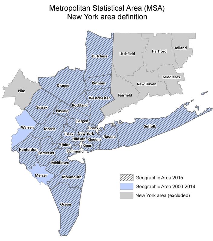
Geographic definition
In this article, the New York area does not entirely overlap the New York–Newark–Jersey City, NY–NJ–PA, MSA,
because of data constraints and an area definition change in 2015.[4] Briefly stated, Pike County in Pennsylvania
does not appear in the 2006–14 datasets and for consistency is excluded from the 2015 dataset. In addition,
Mercer and Warren Counties in New Jersey are included in the 2006–14 datasets and do not appear in the 2015
2U.S. BUREAU OF LABOR STATISTICS MONTHLY LABOR REVIEW
dataset. (See appendix B for a New York area map.) Note that rather than “Rest of the United States,” this article
examines the United States as a whole to allow for comparisons with other studies and statistics that are reported
for the entire nation.
The Great Recession
The Great Recession, from December 2007 to June 2009, was the longest recession in the United States since
World War II to date.[5] Even after the recession officially ended, the national unemployment rate continued to rise,
peaking at 10.6 percent in January 2010. In fact, not until May 2016 did the economy attain its prerecessionary
unemployment rate of 4.5 percent.[6] As table 1 shows, although the United States and the New York MSA were
clearly affected by the recession, some differences occurred in the timing and severity, as demonstrated by major
recessionary indicators.[7] Between 2006 and 2009, in both the nation and the New York MSA, the economy was
marked by falling employment and the near doubling of the unemployment rate. Specifically, the national
unemployment rate jumped from 4.6 percent to 9.3 percent and the MSA unemployment rate increased from 4.5
percent to 8.6 percent. As is characteristic of a recession, real gross domestic product (GDP) fell in the United
States, and not until 2010 did the real GDP begin to recover. Real GDP fell in the New York MSA as well, but the
recovery began earlier, in 2009.[8] In the MSA, real (that is, inflation-adjusted) annual pay also declined, and in the
United States as a whole, the poverty rate increased. (See table 1.)
Table 1. Five measures of economic health, United States and New York–Newark–Jersey City, NY–NJ–PA
MSA, by selected years
United States New York MSA
Measure
2006 2009 2015 2006 2009 2015
Unemployment rate 4.6 9.3 5.3 4.5 8.6 5.3
Employment (in thousands) 133,834 128,608 139,492 8,128 7,979 8,919
Real pay (in dollars) 50,008 50,333 52,942 72,475 70,164 72,763
Poverty rate 12.3 14.3 13.5 12.8 12.8 14.1
Real GDP (in billions of dollars) 15,315.90 15,236.30 17,390.30 1,291.80 1,300.10 1,459.50
Note: Data are current as of October 20, 2021. GDP = gross domestic product, and MSA = metropolitan statistical area.
Source: The unemployment rates are from U.S. Bureau of Labor Statistics (BLS) Current Population Survey for the United States and Local Area
Unemployment Statistics for the New York MSA; employment is from BLS, Quarterly Census of Employment and Wages; real pay dollars are from BLS,
Quarterly Census of Employment and Wages, adjusted with the United States and New York–Newark–Jersey City Consumer Price Index for All Urban
Consumers in 2015 dollars; U.S. poverty rates are from U.S. Census Bureau, Current Population Survey, Annual Social and Economic Supplements; New
York MSA poverty rates are from American Community Survey, 1-year estimates (starting in 2013, the New York MSA included two additional counties
[Dutchess County and Orange County in New York]); and real GDP data are from the U.S. Bureau of Economic Research Analysis, GDP in chained 2012
dollars.
SNAP description
Known as the Food Stamp Program before 2008, SNAP is the nation’s largest nutrition assistance program that
provides a hunger safety net to eligible low-income individuals, who would otherwise be unable to afford basic
nutrition.[9] SNAP benefits can be used to buy food for household consumption from approved grocery stores
(excluded are hot food, food that will be eaten in the store, vitamins and medicines, alcohol, tobacco, pet food, and
other nonfood items).[10] SNAP benefits are transferred to households via electronic debit cards, known as
Electronic Benefit Transfer (EBT) cards. Participants can use the EBT cards in approved retail stores and farmers’
3U.S. BUREAU OF LABOR STATISTICS MONTHLY LABOR REVIEW
markets nationwide to buy eligible food products, which for the purposes of this study are recorded under food-at-
home expenditures.
Before the Great Recession, there was a steady rise in SNAP participation. In 2006 (the first year of this study),
SNAP participation stood at 26.5 million. (See chart 1.) Beginning in 2008, the first full year of the recession,
participation rose rapidly, reaching a postrecession peak of 47.6 million in 2013, when enrollment rates and costs
were the highest in the program history. In the 2013 peak year, 15 percent of the population received SNAP
benefits and total program costs were $79.9 billion.[11] From 2013 to 2016, participation gradually declined. (See
chart 1.)
In the 2016 fiscal year, 44.2 million individuals in 21.8 million households participated in the program; monthly
benefits averaged $125.40 per individual and $254.61 per household.[12] These levels are down from the peak
nominal benefit levels reported in 2010 through 2013 when benefits were supported by the American
Reinvestment and Recovery Act (ARRA) of 2009.[13] (See appendix A.) In real terms, the average monthly benefit
level was highest in 2010 at $150 per person.[14]
Within the continental United States, SNAP has uniform eligibility requirements and benefit levels.[15] (See
appendix A, tables A-2 and A-3.) Households are eligible for the program if their net income is at most 100 percent
and their gross income is up to 130 percent of the federal poverty level.
4U.S. BUREAU OF LABOR STATISTICS MONTHLY LABOR REVIEW
Households that include individuals 60 or older or disabled individuals who are unable to buy and prepare food are
eligible if gross household income from other members does not exceed 165 percent of the federal poverty level.
Administering states have some authority to set up categorical eligibility for certain classes of households, such as
those that include individuals who are older or disabled and who also receive Supplemental Security Income (SSI)
or those who are already eligible for other types of public assistance benefits.[16] Some states, including New
York, have established categorical eligibility for SSI recipients who are older or disabled and have no other source
of income. In addition, the SNAP allows for states with high unemployment to apply for a time-limit waiver for able-
bodied adults without dependents (ABAWDs), who are normally eligible for SNAP for no more than 3 months in
any given 36-month period, unless certain work or training requirements are met.[17]
The specifics of program eligibility, allowable deductions from income, and benefit levels are revisited
approximately every 5 years in what is commonly known as the Farm Bill. The 10-year period studied
encompasses three separate Farm Bills—2006, 2008, and 2014—as well as ARRA. (See appendix A for details.)
Data
Consumer Expenditure Surveys
The principal data source for this article is the Consumer Expenditure Surveys (CE), collected for BLS by the
Census Bureau. Published annually in a consistent format since 1984, the CE provide information on the buying
habits of consumers in the United States, including detailed information on their expenditures, income sources,
and demographic characteristics. Most CE data are collected at the consumer unit (CU) level, while some (such as
demographic characteristics) are collected for members therein. Unlike the term “household”—which, according to
the Census Bureau, “consists of all the people who occupy a housing unit”—the term “CU” is flexible and can refer
to a family or nonrelated individuals living together, but only if they are sharing key expenses.[18] For example, if
roommates share the responsibility of most expenditures (share 2 of the 3 major expenses: housing, food and
other living expenses), they compose one household and are classified as a single CU. If most expenditures are
made individually, then each roommate represents a separate CU with its own reference person within a single
housing unit.[19] Regardless, for the purposes of this article, “household” and “CU” are used interchangeably.
The two components of CE are the quarterly Interview Survey and the weekly Diary Survey. Whereas purchases
for major and/or recurring items are documented in the Interview Survey, purchases for minor or often bought
items are recorded in the Diary Survey.[20] Combined, the Interview and Diary Surveys provide a detailed picture
of the purchasing habits and expenditures for the nation.
This article uses public use microdata from the 2006–15 CEDs. Data are collected in several stages. In an initial
interview, a Census Bureau representative collects CU demographic and income data, either by telephone or in
person. The interviewer requests that each night respondents log purchases and the amount spent—including all
applicable sales and excise taxes—by all CU members. Detailed expenditure data are captured in one booklet per
week over 2 consecutive weeks. The 2 weeks of data are treated as statistically independent of each other.[21]
The CE are well suited to this project for several reasons. First, detailed expenditure data are linked to key
demographic and income characteristics at the CU level. Second, Diary Survey data provide detailed food-at-home
expenditures. Third, the dataset includes identifiers for the New York area, the geographic area of interest in this
article. Specifically, the New York area accounts for 7.2 percent of the final sample of CUs nationwide for the 10
5U.S. BUREAU OF LABOR STATISTICS MONTHLY LABOR REVIEW
years of data. Fourth, the sample size is large, an average of more than 13,000 observations annually between
2006 and 2015, allowing for analysis at the local-area level.
Unemployment and Consumer Price Index data
In addition, this study merges in 2006–15 external BLS data on state unemployment rates from the Local Area
Unemployment Statistics, national unemployment rates from the Current Population Survey, and BLS Consumer
Price Index (CPI) data. Where the state designator was not available in the CE, state unemployment could not be
matched. In these cases, the national unemployment rate was used.[22] To have a consistent measure over the
10-year period and facilitate comparisons over time, we used the U.S. city average CPI for All Urban Consumers to
convert income and expenditures to constant 2015 dollars. We used the index for all items to convert CU income
and used the index for food at home to convert food-at-home expenditures and SNAP benefits.[23]
Variable description
Food-at-home expenditures—a key variable used as the dependent variable in the regression analysis—record
self-reported weekly expenditures (that is, expenditures collected daily in the Diary Survey over the course of a
week) on food purchases from grocery stores and similar venues.[24] This variable excludes food prepared by the
CU on out-of-town trips, as trip expenditures are only collected in the Interview Survey. Another key variable,
SNAP participation, is also self-reported and indicates whether any member of the CU received SNAP benefits in
the past 12 months.[25] In this analysis, annual income comes from two sources: income from SNAP benefits, if
any, and imputed pretax income from all other sources (based on the past 12 months). This annual income is then
converted to a weekly estimate.[26]
Food expenditures are influenced by CU size, because larger CUs have more mouths to feed. In addition, when
members are added to a household, economies of scale may be realized. Similarly, children and adults may add to
CU food spending in differing proportions, creating adult–child equivalency issues. Because of these issues,
household composition was thoroughly explored in this article. Specifically, households were subdivided into the
following categories: one adult; one adult, one child; one adult, two children; two adults; two adults, one child; two
adults, two children; and all other. Age of the reference person was also divided into the following age groups: 16–
34, 35–49, 50–61, and 62 and older.[27] Education in the CU is defined as the highest degree obtained between
the reference person and the spouse (less than high school, high school, some college, bachelor’s degree, and
more than bachelor’s degree).
The Great Recession is a binary variable, which equals 1 if the diary start date falls between December 2007 and
June 2009 and zero otherwise. Similarly, the prerecession binary variable captures the records with a diary start
date before December 2007 and with the postrecession binary variable after June 2009. Appendix C, table C-1,
provides detailed information on CE variable names and descriptions.
Sample description
Out of the initial 136,467 observations in the combined 2006 through 2015 dataset, a total of 11,680 records (8.6
percent of the sample) were dropped. Of the deleted records, 6,465 were dropped because of missing SNAP
participation status. Additional records were dropped because of
· missing or negative imputed income before tax (SNAP income and income from all other sources),
6U.S. BUREAU OF LABOR STATISTICS MONTHLY LABOR REVIEW
· negative calculated pretax income from all other sources,
· inconsistency between the self-reported SNAP participation status and the imputed values for SNAP
benefits received (that is, CUs reporting SNAP participation with a zero value imputed for SNAP benefits
received), and
· age of the reference person below 16 years.
The resulting sample size was 124,787 CU observations. See table 2 for sample sizes for all CUs and for CUs
with SNAP beneficiaries in the United States and New York area by year. Over this period, the yearly sample
size varied from a low of 10,766 in 2015 to a high of 13,379 in 2006. (See table 2.)
Table 2. Consumer unit count by geographic area and SNAP status, 2006–15
United New York United States United States non- New York – area New York–area non-
Year
States area SNAP SNAP SNAP SNAP
2006–
124,787 8,931 10,496 114,291 817 8,114
15
2006 13,379 847 749 12,630 60 787
2007 12,634 912 659 11,975 58 854
2008 13,027 927 744 12,283 63 864
2009 13,319 992 1,030 12,289 93 899
2010 13,006 998 1,122 11,884 83 915
2011 12,639 1,011 1,224 11,415 83 928
2012 12,453 872 1,262 11,191 86 786
2013 11,289 786 1,288 10,001 97 689
2014 12,275 904 1,322 10,953 110 794
2015 10,766 682 1,096 9,670 84 598
Note: SNAP = Supplemental Nutrition Assistance Program.
Source: U.S. Bureau of Labor Statistics Consumer Expenditure Diary Surveys, 2006–15.
Methodology
Since SNAP benefits can only be used to make food-at-home purchases, the focus of the analysis is on food-at-
home expenditures. The discussion begins with a trend analysis of weekly food-at-home expenditures and
socioeconomic and key demographic characteristics. The analysis by geography and SNAP participation status
over the 10-year period examines the following four groups: New York area SNAP, New York area non-SNAP,
United States SNAP, and United States non-SNAP. Next, summary statistics are presented for the combined 10
years of data, subdivided by geography and SNAP status. In the subsequent regression analysis, a Box-Cox
transformation was used to normalize the food expenditure and income data.[28] In addition, we present results
from logistic models for whether or not households incurred food-at-home expenditures in the survey week for the
United States and the New York area. These models examine the relationship with SNAP status, SNAP income,
income from other sources, and household composition, while controlling for demographics, socioeconomic
factors, home and vehicle ownership, region of residence, unemployment rate, and recessionary period. Also given
are ordinary least squares (OLS) regression results for the relationship of key factors with dollars spent on food at
home among the households that went shopping. Finally, we report marginal propensities to consume (MPCs) and
7U.S. BUREAU OF LABOR STATISTICS MONTHLY LABOR REVIEW
income elasticities to measure consumers’ responsiveness to changes in income from SNAP benefits or cash.
(See appendix D, “Technical notes,” for detailed explanations.)
SNAP and unemployment trend analysis
Chart 2 shows the SNAP participation rate at the CU level and BLS unemployment statistics for the United States
and the New York area. In 2006, 5.6 percent of CUs nationally reported SNAP participation. As expected, with the
increase in unemployment, the percentage of CUs reporting having received SNAP benefits rose. In 2009, when
the Great Recession officially ended, SNAP participation stood at 7.7 percent. But even as national unemployment
rates began to gradually decline, SNAP participation continued to rise, peaking at 11.4 percent in 2013. By 2015,
SNAP participation stood at 10.2 percent, well-above prerecession levels. The New York area followed a similar
pattern, with an overall rising trend in SNAP participation following the onset of the Great Recession. SNAP
participation in the local area reached a peak of 12.3 percent in 2013 and 2015.
Food-at-home expenditure trends
For the charts that follow, trends for four CU groupings will be examined: United States SNAP, United States non-
SNAP, New York area SNAP, and New York area non-SNAP. (Note that in the case of New York area SNAP CUs,
some volatility may be attributed to the relatively small yearly sample sizes, between 58 and 110 CUs. See table
2.) Food-at-home expenditures are analyzed for all CUs (chart 3A) and for CUs who went shopping in the
8U.S. BUREAU OF LABOR STATISTICS MONTHLY LABOR REVIEW
reference week (chart 3B). As chart 3A shows, New York area SNAP CUs showed the greatest volatility in weekly
food-at-home spending as measured in 2015 dollars over the 10-year period. This group’s expenditures were most
pronounced in 2008—the only full-recession year—and from 2010 to 2011—a postrecession period of elevated
unemployment. Note that ARRA took effect in April 2009, beginning a temporary increase in benefit allotments that
went through March 2014, with 2010 and 2011 marking the first full years of ARRA’s implementation. (See
appendix A for more details on ARRA, income eligibility [table A-2] and benefits [table A-3].) An overall downward
trend occurred in food-at-home expenditures for New York non-SNAP CUs between 2006 and 2015. For the other
groups, food-at-home expenditures stayed largely in the $70 to $80 per-week range.
9U.S. BUREAU OF LABOR STATISTICS MONTHLY LABOR REVIEW
Among the CUs that shopped in the reference week, the expenditure levels are higher because the zero-
expenditure CUs have been removed from the calculations (chart 3B). In this case, both New York area SNAP and
non-SNAP CUs show much volatility in weekly expenditures, whereas United States CUs show a flat trend and
less volatility.
Socioeconomic and demographic trend analysis
To further understand the variation in food-at-home expenditures, we examine the differences in demographic
characteristics among SNAP participants and nonparticipants over the 10-year period. As discussed earlier, these
characteristics are also compared for the New York area and the nation as a whole.
Income
Household income is the main factor in determining SNAP eligibility. (See appendix A, table A-2.) Income eligibility
standards are determined by the federal poverty level and do not vary among the contiguous states. As shown in
chart 4, SNAP beneficiaries’ income (measured in income before tax in 2015 dollars, exclusive of the value of
SNAP benefits) remained essentially unchanged over the 10-year period at roughly $450 a week.
Annual income nationwide for non-SNAP recipients showed a slight but steady decrease beginning in 2007, until
reaching a low in 2013—coinciding with the onset and aftermath of the Great Recession—for an overall loss of 9.5
percent of real income. As expected, for non-SNAP CUs in the New York area, income was consistently higher
10U.S. BUREAU OF LABOR STATISTICS MONTHLY LABOR REVIEW
than their nationwide counterparts and showed much more volatility, dropping noticeably during the Great
Recession. Chart 4 further shows a greater income disparity between SNAP and non-SNAP CUs in the New York
area than in the United States. Non-SNAP CUs earned 3.9 times and 3.2 times the annual income of SNAP CUs,
in the New York area and the United States, respectively.[29] These findings are consistent with the higher
average income in the New York area and with nationally established SNAP eligibility requirements.
Education
The prevalence of bachelor’s degree holders was higher among non-SNAP CUs than SNAP CUs in the United
States and in the New York area. In the United States, a slight upward trend occurred in the percentage of
bachelor’s degree holders for both SNAP and non-SNAP CUs. In the New York area, among non-SNAP CUs, the
proportion of bachelor’s degree holders marked a low point in the recession years of 2008 and 2009 but reached a
10-year peak in 2013, about 4 years after the recession, a typical length of a bachelor’s program. The number of
bachelor’s degree holders increased among SNAP CUs in the New York area during the recession and had great
volatility afterward. (See chart 5.)
11U.S. BUREAU OF LABOR STATISTICS MONTHLY LABOR REVIEW
Age
The aging of the U.S. population is well established. As shown in chart 6, the gradual rising in the average age of
the reference person applies to both SNAP and non-SNAP CUs. Nationwide, SNAP reference persons were
younger than their non-SNAP counterparts, while in the New York area, the average age of the reference persons
in SNAP and non-SNAP CUs broadly coincided.
12U.S. BUREAU OF LABOR STATISTICS MONTHLY LABOR REVIEW
Although the average age of the reference person in SNAP CUs declined during the recessionary period of 2008–
09 for both the New York area and the United States, the drop in the local area was about 4 times larger (5.4 years
of age versus 1.4 years). Given the aging population, this decline in the average age of SNAP CUs during the
recession might be attributed to an increase in participation among younger cohorts, consistent with ARRA’s
suspension of the 3-month SNAP participation limit for ABAWDs. (See appendix A for more details.) Local area
age differences might also be attributed to geographic mobility, such as older participants leaving the area.
However, the cross-sectional nature of the data does not allow a definitive conclusion.
Race
For the race characteristic, we found that SNAP CUs had a higher proportion of Black reference persons than non-
SNAP CUs in both the United States and the New York area. As chart 7 shows, much volatility occurred before,
during, and after the recession in the share of New York area SNAP CUs with a Black reference person, with no
clear trend presenting itself. By contrast, in the United States, a noticeable downward trend occurred since 2011 in
the proportion of SNAP CUs with a Black reference person. Among non-SNAP CUs with a Black reference person,
we see an upward trend in the New York area from 2007 to 2014, whereas in the United States, we see neither a
noticeable trend over the 10-year period nor a recessionary effect.
13U.S. BUREAU OF LABOR STATISTICS MONTHLY LABOR REVIEW
Ethnicity
As chart 8 shows, at the onset of the recession—from 2007 to 2008—the percentage (when rounded) of SNAP
CUs that identified as Hispanic in the local area rose by 15.8 percentage points (from 41.4 percent to 57.1
percent), compared with a 0.7-point increase nationwide (from 22.0 percent to 22.7 percent). After the initial climb
through 2008, the percentage of Hispanic SNAP CUs in the New York area showed high volatility. In the United
States, a slight upward trend is noticeable for SNAP CUs, whereas no clear trend exists for non-SNAP CUs.
14U.S. BUREAU OF LABOR STATISTICS MONTHLY LABOR REVIEW
Housing
A discussion of renting status is relevant, because renters are more likely to be food insecure,[30] and one of the
distinguishing characteristics of the New York area is the high percentage of renters. As expected, among both
SNAP and non-SNAP CUs, renters are more prevalent in the New York area than in the United States (see chart
9). Over the 10-year period, renters among non-SNAP CUs increased 2.8 percentage points in the United States,
coinciding with the increase in foreclosures during and following the Great Recession, more stringent mortgage
eligibility requirements, and changing patterns of household formation.[31] In the New York area, much volatility
occurred in the share of SNAP CUs who rented, reaching a 10-year high in 2008 of 96.8 percent—compared with
the 70.9-percent peak nationwide in 2009.
15U.S. BUREAU OF LABOR STATISTICS MONTHLY LABOR REVIEW
Marital status
In general, because of typically higher household income, married CUs are less likely to be eligible for SNAP
benefits and therefore have lower participation rates than the rates of those not married. In fact, through the 10-
year period, about a quarter to a third of the reference persons in SNAP CUs were married, compared with over
half of non-SNAP CUs. But with the high unemployment rates of the Great Recession, that pattern did not
necessarily hold. In chart 10, no clear upward or downward trend is shown for any group. For the United
States, among SNAP CUs, the percentage of married couples peaked in 2010 at 34.3 percent. This bump may be
explained by high levels of unemployment, which also peaked in 2010. As mentioned earlier, married CUs who lost
earners would be more likely to meet SNAP income eligibility guidelines.
16U.S. BUREAU OF LABOR STATISTICS MONTHLY LABOR REVIEW
Number of adults
As chart 11 shows, over the 10-year period, generally fewer than two adults lived in the CU and SNAP CUs mostly
had fewer adults than non-SNAP CUs. In 2010 and even less in 2014, local area SNAP CUs experienced a
pronounced increase in the average number of adults present. The rise in the number of adults—particularly in
2010, with its peak unemployment—may be due to adult children moving back in with their parents or a rise in
unemployment among spouses making them eligible for SNAP.[32]
17U.S. BUREAU OF LABOR STATISTICS MONTHLY LABOR REVIEW
Number of children
By program design, SNAP participation is more likely among families with children under 18 living in the
household. As chart 12 shows, SNAP-participating CUs had more children compared with non-SNAP CUs. SNAP
CUs had, on average, twice as many children as non-SNAP CUs. Over the 10-year period, there was a slight
downward trend in the number of children in non-SNAP CUs—the largest group. This trend is consistent with an
aging population and declining birth rate. For SNAP CUs, fluctuations followed by a clear downward trend occurred
after 2011. The cross-sectional nature of the data limits our ability to determine the reasons for the fluctuations.
18U.S. BUREAU OF LABOR STATISTICS MONTHLY LABOR REVIEW
Summary statistics
Table 3 displays the summary statistics for the pooled 10-year sample, first by geography (United States and New
York area) and then by geography and SNAP status (United States SNAP and non-SNAP and then New York area
SNAP and non-SNAP). Table 3 also shows mean comparisons—based on Satterthwaite t-test for continuous
variables and t-test of proportions for binary variables[33]—for analyzing statistically significant differences
between these groups (SNAP versus non-SNAP). Since the New York area is a subset of the United States, one
cannot conduct t-tests between these geographies. Because CE data for the New York area cannot be weighted in
a statistically reliable way, all analyses herein are unweighted. (See “Weighting CE data” in appendix D, “Technical
notes,” for details.)
Table 3. Summary statistics by geographic area and SNAP status, 2006–15
Between 2006 and 2015, 8.4 percent of CUs nationwide and 9.1 percent in the New York area reported receiving
SNAP benefits in the prior 12 months. Weekly food-at-home bills averaged $81.19 (in 2015 dollars) in the United
States and $83.25 in the New York area. SNAP beneficiaries nationwide spent $77.68 per week on food at home,
while local area beneficiaries spent $82.18. (See table 3.)
Not all CUs made food-at-home purchases during the reference week.[34] Among those who did—83.8 percent of
CUs in the United States and 77.1 percent in the New York area—the average bill was $96.89 and $107.94,
respectively. As the raw data show, among the weekly shoppers, SNAP-participating CUs spent about $7.00 less
19U.S. BUREAU OF LABOR STATISTICS MONTHLY LABOR REVIEW
compared with non-SNAP CUs nationwide, $90.38 versus $97.51, and nearly $16.00 less in the local area, $93.64
versus $109.60.
As this article shows, household composition is an important factor to consider when food-at-home expenditures
are analyzed, both for SNAP and non-SNAP households. Single-adult CUs (one adult, zero children) are among
the largest household configurations, comprising 23.5 percent of SNAP CUs and 28.7 percent of non-SNAP CUs
nationwide. However, in the New York area, single-adult SNAP and non-SNAP CUs exist in similar proportions,
29.6 percent and 28.5 percent, respectively. Two-adult CUs (two adults, zero children), another common
arrangement, show the greatest variation by SNAP status. In the United States, they comprise 13.7 percent of
SNAP CUs and 32.7 percent of non-SNAP CUs. In the New York area, the corresponding percentages are 14.4 for
SNAP and 30.2 for non-SNAP CUs.
As the t-tests show, many significant differences were found between the characteristics of SNAP and non-SNAP
CUs within the two geographies. For example, SNAP CUs in the local area earned 25.7 percent of the non-SNAP
CUs’ income from all sources other than SNAP, as compared with 31.0 percent nationwide (both statistically
significantly different at the 1-percent level). Renters are significantly more prevalent in SNAP CUs than non-SNAP
CUs in the New York area (90.7 percent versus 38.3 percent) and the United States (68.1 versus 28.2 percent).
Another New York phenomenon is low car-ownership rates. In the local area, among SNAP CUs, 75.4 percent do
not own a vehicle as compared with 33.9 percent among non-SNAP CUs. In the United States, the difference is
less pronounced (33.6 percent versus 13.0 percent, respectively). Notable exceptions to the statistical differences
found by the t-test comparisons were food-at-home spending and age for SNAP and non-SNAP CUs in the local
area. For example, in the New York area, both SNAP and non-SNAP CU reference persons were about 50 years
old, whereas in the United States, SNAP CUs were 5 years younger than non-SNAP CUs (45.1 percent versus
50.1 percent).
Regression analysis
As noted in the previous section, measurable differences can be found in the demographic characteristics of SNAP
and non-SNAP CUs in the United States and the New York area. Differences in characteristics, such as household
composition, education, and age, can influence food shopping and expenditure patterns. To account for these
differences, we use regression analysis, a powerful tool that ensures comparisons of like characteristics, to
quantify food-at-home expenditures attributable to SNAP status, while controlling for demographic and regional
differences across population groups and economic characteristics (income, unemployment rate, and business
cycle).[35] Specifically, table 4 (A-B) shows the logistic regression results for whether or not food at home was
purchased in the reference week, and table 5 (A-B) displays the OLS results for dollar expenditures among weekly
shoppers. The tables present coefficient estimates and corresponding standard errors from the regression results
for food-at-home expenditures for the United States and the New York area samples. The estimates in both tables
are with respect to the reference group. The reference person of the group was defined as a non-SNAP working
adult, aged 35–49, who was white, non-Hispanic, never married, neither a single male nor single father, a high
school graduate, and a renter with no vehicles and who lived in the Northeast during the Great Recession at the
time of the interview. (The reference group was assigned the most typical characteristics of the New York area
sample, except for household composition, education, and marital status, in which case a single, never married
person with a high school diploma was chosen as a useful benchmark for further comparisons.)
20U.S. BUREAU OF LABOR STATISTICS MONTHLY LABOR REVIEW
Table 4A. Income, Box–Cox transformation of income, and predicted probability
of food-at-home purchases for SNAP and non-SNAP consumer units incurring
food-at-home expenditures in the reference week, by geographic area, 2006–15
Table 4B. Logistic regression results for consumer units incurring food-at-home
expenditures in the reference week, by geographic area, 2006–15
Table 5A. Income, Box–Cox transformation of income, and predicted food-at-
home expenditures for SNAP and non-SNAP consumer units incurring food-at-
home expenditures in the reference week, by geographic area, 2006–15
Table 5B. Ordinary least squares regression results for food-at-home
expenditures for consumer units incurring expenditures in the reference week,
by geographic area, 2006–15
According to table 4 (A-B), receipt of SNAP benefits has a significant and positive relationship with the probability
of buying food at home in the reference week nationwide but not in the New York area. In the United States, the
predicted probability of food shopping in the reference week for the reference group as just described was 61.3
percent. For non-SNAP CUs nationwide, adding a child (one adult, one child) to the specified reference group
increases the probability of buying food at home by 4.6 percentage points to 65.9 percent. Adding a second child
(one adult, two children) increases that probability by 9.8 percentage points over the reference group. When an
adult is added to the mix (two adults, one child), the probability of food-at-home shopping of non-SNAP CUs is 8.3
percentage points higher than that of the reference group, while adding yet another child (two adults, two children)
raises the probability by 8.7 percentage points.
SNAP CUs nationwide exhibit a different pattern. If we assume the attributes of the reference group and only
consider SNAP households, the predicted probability of buying food at home in the reference week increases by
almost 15 percentage points to 76.2 percent. (See table 4 [A-B].) In contrast to non-SNAP CUs, adding a child to a
SNAP CU decreases the probability of making weekly food-at-home purchases by 1.6 percentage points. Adding a
second child decreases the probability even more, by 2.3 percentage points over the reference group in SNAP
households. When an adult is added to this mix, the probability becomes positive, at 2.5 additional percentage
points for two adults-one child CUs and 5.5 percentage points for two adults-two children CUs. The change of the
probability from negative to positive when an adult is added to a SNAP CU suggests that SNAP CUs may be
taking advantage of built-in childcare with the second adult in the household.
In the New York area, table 4 (A-B) shows the reference group had a 54.6-percent probability of making food-at-
home purchases in the reference week. However, neither altering household composition nor receiving SNAP
benefits were significantly associated with that probability, except for two adults-two children CUs, in which the
probability increased by 7.9 percentage points for non-SNAP CUs (to 62.5 percent) and 23.9 percentage points for
SNAP CUs (to 89.9 percent).
Vehicle ownership is among the variables with the largest influence on the probability of weekly food-at-home
shopping. Compared with CUs with no vehicles, having a vehicle is associated with a higher probability of 22.6-
percentage-points of making weekly purchases for non-SNAP CUs and 15.1 percentage points for SNAP CUs
nationwide. In the local area, although vehicle ownership is much lower, having a vehicle is linked to an increase of
21.3 and 17.6 percentage points in the probability of weekly food-at-home shopping. (See table 4 [A-B].) Having a
21U.S. BUREAU OF LABOR STATISTICS MONTHLY LABOR REVIEW
second vehicle is associated with a further increase in the probability. The large estimates of vehicle ownership
suggest that the convenience of having a car is associated with changes in CU shopping behavior.
To examine the influence of the Great Recession, in the regressions, we separate periods into before, during, and
after the recession and use the recessionary period (December 2007–June 2009) as the reference period. Before
the recession, CUs nationwide and in the local area were more likely to make weekly food shopping trips
compared with those made during the recession. Postrecession, CUs nationwide were less likely to make weekly
food shopping trips, whereas CUs purchasing behavior in the local area was not significantly different. These
findings reveal the importance of studying changes in purchasing behavior in light of the Great Recession.
Table 5 (A-B) shows the OLS regression results for weekly food-at-home expenditures in 2015 dollars for CUs
nationwide and in the local area.[36] In contrast to table 4 (A-B), which analyzes the full sample, table 5 (A-B)
focuses on the CUs that made food-at-home purchases in the reference week. Table 5 (A-B) shows that in the
United States, the reference group of non-SNAP CUs spent an average of $43.20 per week on food at home.
When adding positive SNAP status, we found that CUs spent an additional $7.71 per week, for a total of $50.91. In
the New York area, non-SNAP CUs spent $40.02 and SNAP CUs spent $62.16. SNAP participants, on average,
spent more than nonparticipants on weekly food-at-home purchases—up $7.71 in the United States and up $22.14
in the New York area. When we accounted for differences in characteristics, SNAP participation clearly increased
food-at-home expenditures—a relationship not clear from the raw data shown in table 3, in which the reverse is
true. While table 3 compares the inherent differences among demographically and socioeconomically diverse
areas, table 5 (A-B) controls for these key factors and thereby isolates the importance of SNAP receipts,
highlighting the benefits of using regression analysis.
One such key factor, household composition, produces significant results across the board. Compared with the
reference group (one adult), adding an adult (two-adult CUs)—the most populous defined household composition
—increased weekly food-at-home spending by $18.56 in non-SNAP CUs and $13.61 in SNAP CUs nationwide and
by $17.55 and $8.42, respectively, in the New York area. In all cases, adding a member to the household resulted
in less than doubling of food-at-home expenditures. For example, in the United States, where a one-adult SNAP
CU spent on average $50.91 per week, adding a second adult increased the weekly food purchases by $13.61
(26.7 percent). The disproportionate increase in expenditures when a second adult is added to the household (that
is, less than doubling of expenditures when doubling the household size) may indicate economies of scale for
food-at-home purchases. However, other explanations are possible, such as substituting for higher or lower priced
food or buying more food away from home. Adding children increased food-at-home expenditures nationwide but
produced mixed results in the local area.
Compared with the recessionary period, consumers nationwide spent less on food at home after the recession,
down $1.16 for non-SNAP CUs and down $1.31 for SNAP CUs. In the New York area, both prerecessionary and
postrecessionary spending periods were not statistically different from the recessionary period.
Table 6 shows income,[37] MPC (marginal propensity to consume), and income elasticity for SNAP recipients and
nonrecipients in the United States and the New York area. For the purposes of this article, the MPC is defined as
the dollar change in food-at-home expenditures, given a marginal increase ($1) in the SNAP benefit amount or
income from all non-SNAP sources. By contrast, income elasticity is the percent change in food-at-home
expenditures, given an incremental percent (1 percent) increase in the SNAP benefit amount or non-SNAP
income. The two sets of MPCs and elasticity estimates answer two questions (given in table 6): “How much are
22U.S. BUREAU OF LABOR STATISTICS MONTHLY LABOR REVIEW
food-at-home expenditures expected to change given a $1 increase in SNAP benefit amounts?” (table 6, top
panel) and “How much are food-at-home expenditures expected to change given $1 increase in other (non-SNAP)
income?” (table 6, bottom panel). Note that both SNAP income and non-SNAP income, such as income from
earnings or Social Security, can be used for food expenditures in SNAP CUs, whereas only non-SNAP income is
available to non-SNAP CUs.
Table 6. Marginal propensity to consume and income elasticity for the consumer unit, by geographic area,
2006–15
United States CUs New York area CUs
Variable
Non-SNAP SNAP Non-SNAP SNAP
How much are food-at-home expenditures expected to change given an increase in SNAP benefit amount?
Income weekly (in 2015 dollars) 459.84 527.31 439.24 511.17
Income, all sources other than SNAP (in 2015 dollars) 459.84 459.84 439.24 439.24
Income, SNAP (in 2015 dollars) [1] 67.47 [1] 71.93
Predicted food-at-home expenditures for the reference group 42.49 50.91 39.38 62.16
MPC ($1 increase)
MPC for income from all sources other than SNAP 0.011 0.004 0.009 0.008
MPC for income from SNAP [1] 0.042 [1] 0.052
Income elasticity (1% increase)
Elasticity for income from all sources other than SNAP 0.120 0.036 0.104 0.055
Elasticity for income from SNAP [1] 0.056 [1] 0.060
How much are food-at-home expenditures expected to change given an increase in other (non-SNAP) income?
Income, weekly (in 2015 dollars) 527.31 527.31 511.17 511.17
Income, all sources other than SNAP (in 2015 dollars) 527.31 459.84 511.17 439.24
Income, SNAP (in 2015 dollars) [1] 67.47 [1] 71.93
Predicted food-at-home expenditures for the reference group 43.20 50.91 40.02 62.16
MPC ($1 increase)
MPC for income from all sources other than SNAP 0.010 0.004 0.008 0.008
MPC for income from SNAP [1] 0.042 [1] 0.052
Income elasticity (1% increase)
Elasticity for income from all sources other than SNAP 0.124 0.036 0.108 0.055
Elasticity for income from SNAP [1] 0.056 [1] 0.060
[1] Data are not applicable.
Note: CU = consumer unit, MPC = marginal propensity to consume, and SNAP = Supplemental Nutrition Assistance Program.
Source: U.S. Bureau of Labor Statistics Consumer Expenditure Diary Surveys, 2006–15.
In table 6, total weekly income is subdivided into income from SNAP benefits, if any, and income from all sources
other than SNAP. In the United States, SNAP CUs reported $527.31 in actual weekly income—$67.47 from SNAP
benefits and $459.84 from all other sources (as seen in table 3, top and bottom panels). For comparison purposes,
the same value for income from other sources—$459.84—is assigned to non-SNAP CUs, whose SNAP benefit
amount would be zero (top panel). Based on these actual or assigned incomes, the expected weekly food-at-home
expenditures are calculated (with the use of the regression results from table 5 [A-B]) at $50.91 for the SNAP
recipients and $42.49 for nonrecipients (top panel).
23U.S. BUREAU OF LABOR STATISTICS MONTHLY LABOR REVIEW
In the United States, as the MPC estimates show, a $1 increase in non-SNAP income is predicted to increase
food-at-home expenditures by 1 cent (or 10 cents for a $10 increase) for non-SNAP CUs and 0.4 cents (or 4 cents
for a $10 increase) for SNAP CUs (table 6, bottom panel), whereas a $1 increase in SNAP benefits is predicted to
increase food-at-home expenditures by 4.2 cents (or 42 cents for a $10 increase) for SNAP households (top
panel).[38] As the income elasticities show, a 1.00-percent increase in non-SNAP income is expected to produce a
0.12-percent increase in food-at-home expenditures for non-SNAP CUs and a 0.04-percent increase for SNAP
CUs (bottom panel). Both the MPC and income elasticity estimates show that households spent most of the
additional income on consumption categories other than food-at-home expenditures. An increase in neither non-
SNAP income nor SNAP benefits is expected to produce a substantial change in food-at-home expenditures.
When SNAP CUs are considered, a 1.00-percent increase in SNAP benefits (top panel) is expected to increase
food-at-home expenditures by 0.06 percent, only slightly more than the increase from non-SNAP income just
discussed (0.06 percent as compared with 0.04 percent).
The New York area results are similar, with the MPC estimates showing that a $1 increase in non-SNAP income
(table 6, bottom panel) is predicted to increase food-at-home expenditures by 0.8 cents (or 8 cents for a $10
increase) for both non-SNAP and SNAP CUs, and a $1 increase in SNAP benefits (top panel) is predicted to
increase food-at-home expenditures by 5.2 cents (or 52 cents for a $10 increase) for SNAP households. Similarly,
the income elasticities show that a 1.00-percent increase in non-SNAP income (bottom panel) is expected to
produce a 0.11-percent increase in food-at-home expenditures for non-SNAP CUs and a 0.06-percent increase for
SNAP CUs, while a 1.00-percent increase in SNAP benefits (top panel) is expected to increase food-at-home
expenditures by 0.06 percent for SNAP CUs.
To conclude the analysis for table 6, we see little difference between the MPC and income elasticity estimates
when answering the question of how much are food-at-home expenditures expected to change given an increase
in SNAP benefit amounts or other non-SNAP income. This finding suggests that consumers respond similarly to an
income increase from SNAP benefits or other (non-SNAP) sources. The small magnitudes of the MPC and income
elasticity estimates suggest that consumers increase their food-at-home expenditures little when receiving extra
income, regardless of the source. In fact, a $10 increase in either source of income results in an increase in food-
at-home spending on the magnitude of pennies and dimes.
Caveats and data limitations
Several caveats and data limitations exist. First, SNAP has evolved over time. During the 10-year period studied,
eligibility requirements and benefits changed four times under three separate Farm Bills (2006, 2008, and 2014)
and ARRA (2009) (see appendix A). Second, food prices are volatile. Droughts, hurricanes, and changes in
exchange rates and oil prices, among other factors, result in fluctuations in food prices in the United States and
worldwide, which are not accounted for in the article.[39] Third, food consumption behavior is constantly changing
in response to nutrition educational programs and awareness of the importance of a healthy diet. In recent years,
public education programs promoted healthy eating through improved food labeling in grocery stores, added
calorie labeling in restaurants, and reduced consumption of sugary drinks, among other initiatives.[40] Fourth, the
availability of free sources of food may influence food expenditure patterns and no CE data exist on additional food
sources used by CUs. For example, food pantries alone fed 44 million unique clients in the United States in
2013.[41] In addition, some evidence exists that the residents of New York City—who comprise a large part of the
New York area population—were using additional free food services at a higher rate than the nation as a
24U.S. BUREAU OF LABOR STATISTICS MONTHLY LABOR REVIEW
whole.[42] Fifth, the definition of the New York area changed in 2015, because of a change in the MSA as a result
of the 2010 decennial census. (See “Why New York?” section.) Sixth, the United States contains the New York
area. Because the New York area is the most populous MSA in the country with over 7 percent of CUs nationwide,
changes in its area statistics also drive nationwide numbers. Seventh, 8.6 percent of the data were excluded. The
exclusions may not have been random and may have biased some of the results. Finally, although this study
examines food-at-home expenditures, it does not address food-away-from-home spending and its impact on food-
at-home spending. For example, households could eat out more and spend less on food at home. Despite these
caveats and limitations, this article contributes to the literature on CU food consumption patterns in the United
States and local area in light of the Great Recession.
Conclusion
Because of the importance of SNAP and the nation’s largest supplemental nutrition program—and the length of
the Great Recession, this article uses 2006–15 CED data to examine the characteristics of SNAP and non-SNAP
CUs across the United States and the New York area—the nation’s most populous metropolitan area—and the
relationship of these characteristics with weekly food-at-home shopping.
Over the 10-year period studied, about 1 in 12 CUs nationwide (8.4 percent) and 1 in 11 CUs in the New York area
(9.1 percent) reported receiving SNAP benefits in the prior 12 months. As expected, with the increased
unemployment associated with the recession, the percentage of CUs reporting SNAP receipt rose, peaking at 11.4
percent nationwide in 2013 and 12.3 percent in the local area in 2013 and 2015.
Since household income as a percentage of the federal poverty level is the main factor in determining SNAP
eligibility, one would not expect much variation in income among SNAP CUs. When CUs by SNAP status are
compared, non-SNAP CUs outearned SNAP CUs by a factor of 3.2 nationally and 3.9 in the New York area,
suggesting greater income disparity in the local area. The commonly known New York phenomena of high rates of
renting and low rates of vehicle ownership were confirmed by the data. Renters were more prevalent in SNAP CUs
than non-SNAP CUs in the New York area (90.7 percent versus 38.3 percent) and the United States (68.1 percent
versus 28.2 percent). In the case of car ownership, 75.4 percent of SNAP CUs did not own a vehicle as compared
with 33.9 percent of non-SNAP CUs in the local area, and 33.6 percent versus 13.0 percent in the United States,
respectively. Over the 10-year period, Hispanic CUs disproportionately identified as SNAP participants in the
United States (24.3 percent) and New York area (47.7 percent). In the local area, SNAP and non-SNAP CUs
differed little in age (about 50 years old), whereas in the nation, SNAP recipients were about 5 years younger
(ages 45 versus 50).
The trend analysis of the demographic characteristics reveals several recession-related differences between
SNAP CUs and non-SNAP in the United States and the New York area. The overall trend was consistent with an
aging population, except for the recessionary years of 2008-09 when the average age of the reference person in
SNAP CUs dropped (5.4 years locally and 1.4 years nationwide), suggesting that the Great Recession
disproportionately affected the younger population. In addition, SNAP CUs in the New York area showed a marked
increase in the proportion of college graduates during the recession, signifying the far-reaching impact of the
recession even on the educated population. Hispanic CUs were also disproportionately affected by the recession
locally, rising 15.8 percentage points from 2007 to 2008 (from 41.4 percent to 57.1 percent), with a 0.7-point
increase nationwide (from 22.0 percent to 22.7 percent). By 2008, 96.8 percent of local area SNAP CUs were
25U.S. BUREAU OF LABOR STATISTICS MONTHLY LABOR REVIEW
renting—a 10-year high—compared with the 70.9-percent peak reached nationwide in 2009, coinciding with the
increase in foreclosures during and following the Great Recession.
Controlling for pre- and postrecession periods, this article uses regression analysis for the United States and the
New York area to examine the factors that may be correlated with the probability of making weekly food-at-home
purchases (logistic regressions). The analysis proceeds with OLS regressions to estimate food-at-home
expenditures for CUs of varying household composition and other characteristics. Nationwide, SNAP receipt was
significantly and positively related to the probability of making weekly food-at-home purchases: SNAP CUs had a
predicted probability of 76.2 percent and non-SNAP CUs had 61.3 percent. In the local area, the corresponding
probabilities were 66.0 for SNAP and 54.6 for non-SNAP CUs, but SNAP receipt was not significant. One reason
for the lower probability in the New York area is the lower rate of vehicle ownership. In fact, owning vehicles is
associated with one of the largest increases in the probability of making weekly purchases for both non-SNAP and
SNAP CUs, rising by as much as 27.5 percentage points for the New York area and 25.9 percentage points
nationwide (non-SNAP CUs, two-vehicle ownership) and 22.1 and 17.0 percentage points, respectively (SNAP
CUs, two-vehicle ownership).
Although no significant relationship was found between household composition and the probability of going food
shopping in the reference week in the New York area, household composition was among the factors with the
greatest impact nationwide. Adding one or two children to the household is associated with a decrease in the
probability of making weekly food-at-home purchases for SNAP CUs, but the same change in household
composition leads to an increase for non-SNAP CUs. Conversely, adding an adult to the mix (with one or two
children) in SNAP CUs is linked to a higher probability, suggesting that SNAP CUs may be taking advantage of
built-in childcare with the presence of a second adult in the household.
Considering weekly food-at-home expenditures by SNAP status, while controlling for differences in characteristics,
we found that SNAP participants spend more on weekly food-at-home purchases than nonparticipants, which was
not clear from the raw data. As the OLS regression results show, nationwide, the reference group of non-SNAP
CUs spent on average $43.20 per week, whereas SNAP CUs spent $50.91; and in the local area, non-SNAP CUs
spent $40.02 and SNAP CUs spent $62.16. Household composition was by far the most important factor in
determining food expenditure levels, with every household configuration increasing expenditures over the
reference group of a single adult, except for CUs of one adult, one child in the local area. When the recession is
considered, the postrecessionary period was associated with significantly lower spending in the nation and no
significant difference for the New York area. In short, controlling for other characteristics, food-at-home
expenditures remained stable over the business cycle.
The estimates for MPCs and income elasticities by SNAP status indicate that consumers respond similarly to an
income increase from SNAP benefits or other (non-SNAP) sources. The small magnitudes suggest that consumers
increase their food-at-home expenditures by pennies and dimes when receiving an extra $10 of income, whether
from SNAP benefits or other sources. Specifically, as the MPC estimates show, a $10 increase in non-SNAP
income increases food-at-home expenditures by as much as 10 cents (non-SNAP CUs, United States). A $10
increase in SNAP income increases food-at-home expenditures by as much as 52 cents (SNAP CUs, New York
area). Income elasticities show that a 1-percent increase in non-SNAP income results in as much as a 0.12-
26You can also read