EXOPLANETS IDENTIFICATION AND CLUSTERING WITH MACHINE LEARNING METHODS - Aircc Digital Library

Machine Learning and Applications: An International Journal (MLAIJ) Vol.9, No.1, March 2022

 EXOPLANETS IDENTIFICATION AND CLUSTERING
 WITH MACHINE LEARNING METHODS

 Yucheng Jin, Lanyi Yang, Chia-En Chiang

 EECS Graduate Student at University of California-Berkeley, Berkeley, CA, USA

ABSTRACT
The discovery of habitable exoplanets has long been a heated topic in astronomy. Traditional methods for
exoplanet identification include the wobble method, direct imaging, gravitational microlensing, etc., which
not only require a considerable investment of manpower, time, and money, but also are limited by the
performance of astronomical telescopes. In this study, we proposed the idea of using machine learning
methods to identify exoplanets. We used the Kepler dataset collected by NASA from the Kepler Space
Observatory to conduct supervised learning, which predicts the existence of exoplanet candidates as a
three-categorical classification task, using decision tree, random forest, naïve Bayes, and neural network;
we used another NASA dataset consisted of the confirmed exoplanets data to conduct unsupervised
learning, which divides the confirmed exoplanets into different clusters, using k-means clustering. As a
result, our models achieved accuracies of 99.06%, 92.11%, 88.50%, and 99.79%, respectively, in the
supervised learning task and successfully obtained reasonable clusters in the unsupervised learning task.

KEYWORDS
Exoplanets Identification and Clustering, Kepler Dataset, Classification Tree, Random Forest, Naïve
Bayes, Multi-layer Perceptron, K-means Clustering, K-fold Cross-validation

1. INTRODUCTION
Over the past decades, astronomers around the world have been relentlessly seeking for habitable
exoplanets (planets outside the Solar System) with great interest [1]. Some habitable exoplanet
candidates are Kepler-22b, which is 600 light-years away from the Sun with an orbital period of
290 days, that has a possible rocky surface at a temperature of approximately 295K with an active
atmosphere [2]; Kepler-69c, which is 2,700 light-years away from the Sun with an orbital period
of 242 days, that is of super-earth-sized with a smaller gravity of 7.159 m/s², compared to the
earth’s gravity [3]; Kepler-442b, which is 1,194 light-years away from the Sun with an orbital
period of 112 days, that is within the habitable zone of its solar system [4].

How can astronomers discover these exoplanets? The answer is they have devoted a considerable
amount of time, energy, and money to explore the vast universe with specialized equipment, such
as the astronomical telescope. As a result, astronomers collect observed data for further analysis,
while the identification of a potential exoplanet remains a complicated problem. How can we
confirm an observation from some astronomical telescopes is an existent exoplanet but not a false
positive sample?

There are several traditional exoplanet identification techniques, including the wobble method,
direct imaging, gravitational microlensing, etc. Specifically, the wobble method traces exoplanets
via a Doppler shift in the star’s light frequencies caused by its planets; direct imaging uses extra-
terrestrial telescopes to capture images from exoplanets; gravitational microlensing detects the

DOI:10.5121/mlaij.2022.9101 1

Machine Learning and Applications: An International Journal (MLAIJ) Vol.9, No.1, March 2022
distortion of the background light [5]. These traditional methods are expensive, time-consuming,
and sensitive to variation in the measurement. Based on these limitations, our motivation for this
study is to develop a simple, efficient, and economic approach to identify exoplanets. Therefore,
we proposed the idea of using machine learning methods for the identification of exoplanets and
used two datasets, both were collected by NASA, to conduct a three-categorical classification
task (supervised learning) and a clustering task (unsupervised learning).

For the supervised learning task, we used the Kepler dataset consisted of false positive (labelled
as “-1”), candidate (labelled as “0”), and confirmed (labelled as “1”) exoplanet samples to
perform a three-categorical classification. The objective is to achieve a classification accuracy of
more than 95%. We selected and trained four models for this problem: classification tree, random
forest, naïve Bayes, and neural network. As a result, our models achieved accuracies of 99.06%,
92.11%, 88.50%, and 99.79%, respectively.

For the unsupervised learning task, we used another dataset consisted of the confirmed
exoplanets data to do the clustering. The objective is to find exoplanets that are in the same
cluster as the earth. We selected and trained a k-means model for this problem. As a result, our k-
means model partitioned reasonable clusters, and we visualized all exoplanets in the same cluster
as the earth in a star map.

The rest of this paper is organized as follows. Section II summarizes the related work from other
researchers. Before the modelling and inference, we conducted data cleaning, exploratory data
analysis (EDA), feature selection, etc., and these are written in Section III. In Section IV, we
present the detailed experimental setup, including model optimization and optimal parameters.
Section V analyses the results obtained by our models and discusses the meanings of the results.
Finally, Section VI concludes the paper with the significance of this study and future work to be
done.

2. RELATED WORK
NASA’s Kepler Mission devoted years of effort to discover exoplanets. William J. Borucki [6]
summarized how traditional approaches were used in the real-world scientific research to
confirm, validate, and model the discovered exoplanets by Kepler. Natalie M. Batalha [7] stated
that the progress made by the Kepler Mission indicates there are orbiting systems that might
potentially be habitable places for the human beings. Lissauer et al. [8] emphasized the
contribution made by the Kepler Mission and the significance of its data in exoplanets detection.

Based on the Kepler dataset or other similar datasets, there are studies that combine machine
learning methods with exoplanets detection, identification, and analysis. Christopher J. Shallue
and Andrew Vanderburg [9] used a convolutional neural network to process the astrophysical
signals and validated two new exoplanets according to the CNN predictions. Rohan Saha [10]
implemented logistic regression, decision tree, and neural network on the Kepler dataset to find
out the probability of existence of an exoplanet candidate. Maldonado et al. [11] summarized
studies about exoplanet transit discovery with ML-based algorithms. Fisher et al. [12] interpreted
high-resolution spectroscopy of exoplanets with cross-correlations and supervised learning such
as Bayesian neural networks. Basak et al. [13] constructed novel neural network architectures to
explore the habitability classification of exoplanets.

These related studies provided us with precious insights into the data pre-processing, model
training, selection, and inference procedures. We designed our experiment based on these studies
and used some of their results as benchmarks.

 2

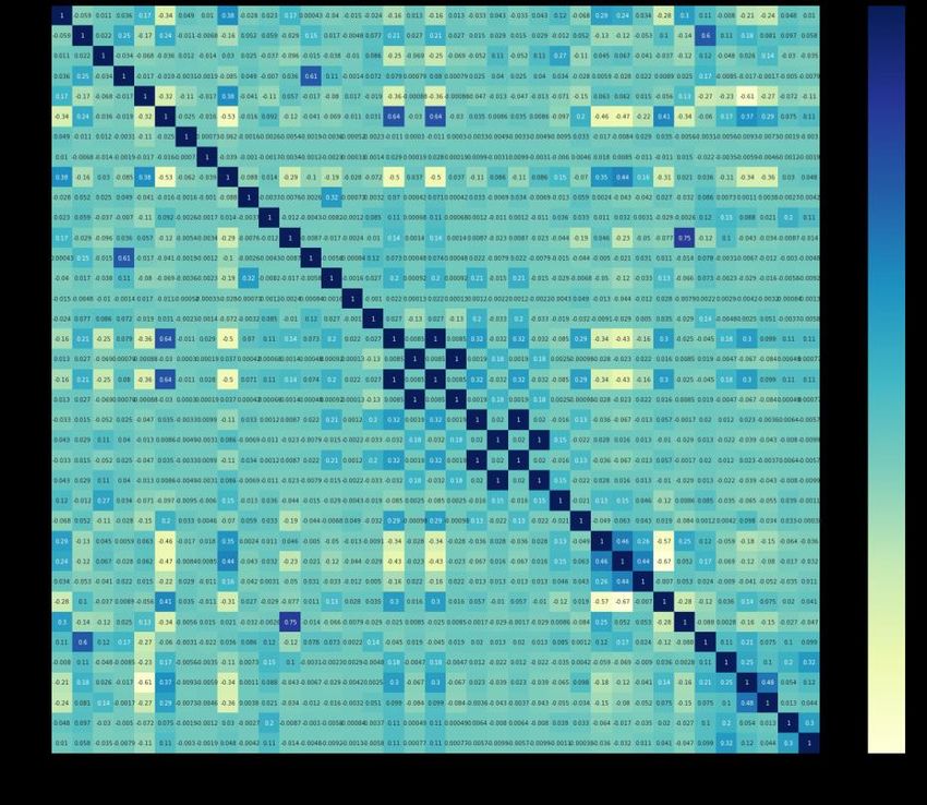
Machine Learning and Applications: An International Journal (MLAIJ) Vol.9, No.1, March 2022

3. DATA PRE-PROCESSING
In this section, we introduce the data pre-processing procedures involved in this study and a short
description of the datasets.

3.1. Dataset Description

The first dataset (the Kepler dataset) in this study is collected by NASA from the Kepler Space
Observatory. In 2009, NASA launched the Kepler Mission, an effort to discover exoplanets with
the goal of finding potentially habitable places for human beings [14]. The mission lasted for
over nine years with remarkable legacies—a total number of 9,564 potential exoplanets are
contained in the Kepler dataset, each associated with features that indicate the characteristics of
the detected “exoplanet”.

Among these features, there is a categorical variable which we selected as the target variable,
koi_disposition, with three possible values, “CONFIRMED” (labelled as “1”), “CANDIDATE”
(labelled as “0”), and “FALSE POSITIVE” (labelled as “-1”). If an exoplanet is
“CONFIRMED”, its existence has been confirmed, and is associated with a name recorded by
kepler_name variable; if an exoplanet is “CANDIDATE”, its existence has not been proven yet;
if an exoplanet is “FALSE POSITIVE”, it has been proven a false positive observation. There are
totally 2,358 confirmed exoplanets, 2,366 candidate exoplanets, and the rest 4,840 exoplanets are
false positive. We used the Kepler dataset for classification, the supervised learning task.

The second dataset (the confirmed exoplanets dataset) contains stellar and planetary parameters
of the confirmed exoplanets [15]. These observations are worldwide, not solely from the Kepler
Mission. Crucial parameters include radius, mass, density, temperature, etc. There are totally
4,375 confirmed exoplanets in this dataset, some were originally discovered by the Kepler Space
Observatory, the rest were originally found by other space observatories. We used the confirmed
exoplanets dataset for clustering, the unsupervised learning task.

3.2. Data Cleaning

The first step of data cleaning was to calculate the proportion of empty entries in each column.
We excluded columns with a large proportion of empty data. Then columns with a small fraction
of empty data were manually selected and the empty entries in the preserved columns were filled
with proper values. Finally, some data were dropped if they had empty values after data cleaning.

3.3. Exploratory Data Analysis (EDA)

Before feature selection and model construction, exploratory data analysis (EDA) is necessary to
facilitate the data analysis process and make it easier and more precise [16]. In this study, EDA
was carried out to obtain an intuitive and high-level understanding of the datasets.

3.3.1. Correlation Analysis

We first conducted correlation analysis to identify highly correlated variables and reduce data
redundancy and collinearity. The correlation matrices of the two datasets are shown in Fig. 1 and
Fig. 2. Both the x-axis and y-axis of Fig. 1 and Fig. 2 are features, and the entry values represent
the correlation coefficients between pairs of features. These two figures are symmetric, because
the correlation coefficient between a variable X and another variable Y follows Corr(X, Y) =
Corr(Y, X). In addition, the diagonal from top left to bottom right is solely consisted of 1’s, since

 3

Machine Learning and Applications: An International Journal (MLAIJ) Vol.9, No.1, March 2022
for each variable X, Corr(X, X) = 1. For a pair of variables, the larger the correlation coefficient
is, the higher the collinearity is; therefore, features with one or more high correlation coefficients
were eliminated by us.

 Figure 1. Correlation Matrix of the Kepler Dataset

 4

Machine Learning and Applications: An International Journal (MLAIJ) Vol.9, No.1, March 2022

 Figure 2. Correlation Matrix of the Confirmed Exoplanets Dataset

3.3.2. Univariate Analysis

Then univariate analysis was performed to visualize the distribution of each variable.

 Figure 3. Count Plots of the Binary Variables of the Kepler Dataset

 5

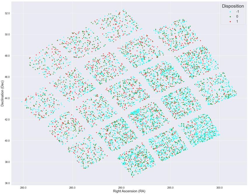
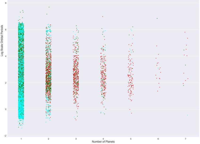
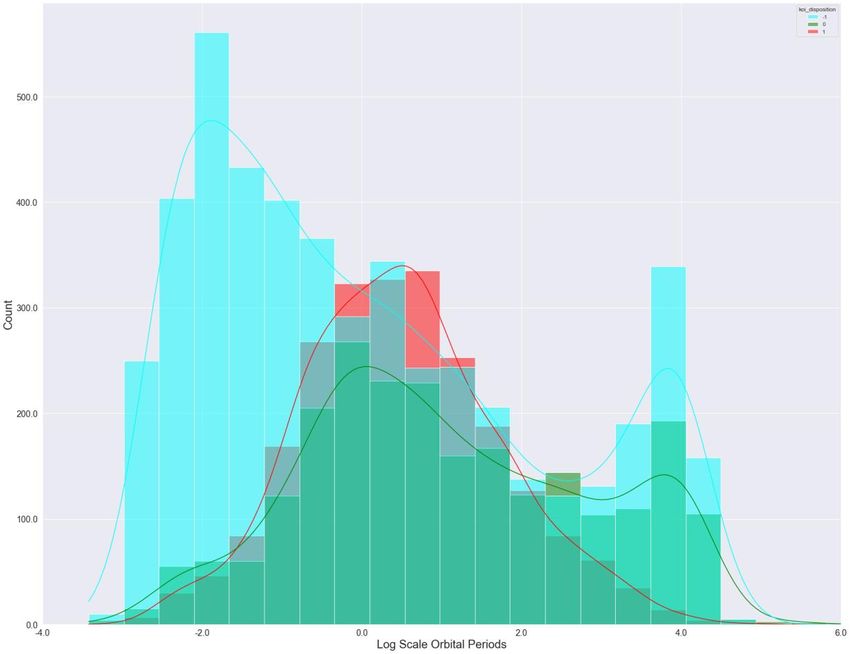
Machine Learning and Applications: An International Journal (MLAIJ) Vol.9, No.1, March 2022

 Figure 4. Histogram of the Log Scale Orbital Periods of the Kepler Dataset

Fig. 3 shows the count of each binary variable in the Kepler dataset, which gives the distribution
of four binary characteristics (non-transit-like, stellar eclipse, centroid offset, ephemeris match
indicates contamination) of the exoplanet candidates.

Fig. 4. is a histogram that indicates the relationship between an important feature, the log scale
orbital period, and the target variable. From Fig. 4, the confirmed exoplanets follow a Gaussian
distribution with respect to the log scale orbital period in the range between -2 and 4. If the value
of the log scale orbital period is too high or too low, the candidate is more likely to be a false
positive observation.

3.3.3. Bivariate Analysis

Finally, we used bivariate analysis to investigate the pairwise relationship between different
features and observe how they affect the target variable.

Fig. 5 is a star map of the exoplanet candidates. In this star map, each pair of celestial coordinates
is measured by right ascension (RA), the celestial coordinate that represents longitude, and
declination (Dec), the celestial coordinate that represents latitude [17]. Fig. 5 demonstrates that
there is no strong correlation between the target variable and coordinates, because for every target
value, these is no clear cluster of exoplanets shown in Fig. 5.

Fig. 6 is a categorical plot of the log scale orbital period versus number of planets in the
exoplanet candidate’s solar system. The result shows that false positive samples are most likely to

 6

Machine Learning and Applications: An International Journal (MLAIJ) Vol.9, No.1, March 2022
have just one or two planets in their solar system. With a higher number of planets in a
candidate’s solar system, the probability of it being a real exoplanet is also higher.

 Figure 5. Star Map by Right Ascension (RA) and Declination (Dec)

 Figure 6. Categorical Plot of the Log Scale Orbital Period versus Number of Planets

 7

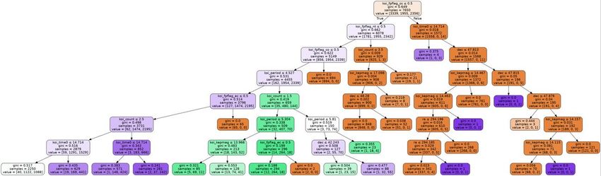
Machine Learning and Applications: An International Journal (MLAIJ) Vol.9, No.1, March 2022
3.4. Feature Selection

Based on the correlation heatmaps, we excluded variables that have high correlation coefficients
with one or more other input features or have a low correlation coefficient with the target
variable. For example, variables that store the deviation of observations, such as koi_period_err
(error of the orbital period) and koi_time0_err (error of the transit epoch), are highly dependent
on the observed values (orbital period and transit epoch). Therefore, we just kept variables that
store the observed values but abandoned variables that record deviation. Some preserved features
are listed in Table 1.

 Table 1. Examples of Preserved Features after Feature Selection

 Variable Dataset Meaning Description
 Kepler name in the form of “Kepler-” plus a
 kepler_name Kepler Kepler Name number and a lower-case letter (e. g. Kepler-
 22b, Kepler-186f)
 Non-Transit-Like 1 means the light curve is not consistent with
 koi_fpflag_nt Kepler
 Flag that of a transiting planet
 koi_period Kepler Orbital Period Measured in days and is taken in log scale
 Number of Number of exoplanet candidates identified in
 koi_count Kepler
 Planets a solar system
 Confirmed Measured in Jupiter Radius
 pl_radj Planet Radius
 Exoplanets
 Confirmed Measured in Jupiter Mass
 pl_bmassj Planet Mass
 Exoplanets
 Confirmed Distance to the planetary system in parsecs
 sy_dist Distance
 Exoplanets

4. EXPERIMENTAL SETUP
In this section, we discuss the model training process in detail with optimization and parameters.
The training process was divided into two parts, training models for classification, and training
the k-means model for clustering. For these two parts, we used the Kepler dataset and confirmed
exoplanets dataset, respectively. For the supervised learning task, we used decision tree, random
forest, naïve Bayes, and neural network. For the unsupervised learning task, we used k-means
clustering.

4.1. Classification Tree

The reason why we chose the decision tree model is that it can split data with classification rules
based on the highest information gain, Info Gain = Entropyparent - Entropychildren. In a
classification tree model, each internal node represents a sample to be split, and each leaf node
represents a class label, or prediction.

We implemented the classification tree model using DecisionTreeClassifier from scikit-learn
library and optimized its performance with different parameters. We set the minimum number of
samples required to split an internal node from 2 to 100 and maximum depth of the tree from 1 to
20, then we selected the parameters that maximized accuracy. As a result, the optimal minimum
number of samples required to split an internal node is 53 and maximum depth of the tree is 7.
Finally, we visualized the optimal decision tree using Graphviz. The optimal decision tree is
shown in Fig. 7 in the next section.

 8

Machine Learning and Applications: An International Journal (MLAIJ) Vol.9, No.1, March 2022
4.2. Random Forest

Random forest combines multiple decision trees together at the training time. As a result, these
decision trees form an ensemble which predicts the class category using the label with the most
votes. For example, in a random forest of 9 decision trees, if 6 predict 1, then the random forest
outputs 1. Customized rules might be applied to break the tie.

We implemented the random forest model using RandomForestRegressor from scikit-learn
library. We optimized the number of trees in the forest by setting this parameter from 20 to 1000
with a step size of 20. As a result, the highest accuracy was obtained when the number of trees is
40.

4.3. Naïve Bayes

Naïve Bayes applies Bayes’ theorem under the assumption that features are independent. It’s a
simple probabilistic approach to conduct the classification task. For features X1, X2, …, Xn and
classes C1, C2, …, Cm, Naïve Bayes (x1, … xn) = argmax ( = ) ∏ =1 ( = | = ).
 
We implemented the naïve Bayes model using ComplementNB from scikit-learn library. Before
training the naïve Bayes classifier, we standardized input features, encoded the target variable as
a one-hot vector, and set each prior as the proportion of each class in the sample space.

4.4. Multilayer Perceptron

Neural network is another machine learning model that is widely used in classification problems.
In a neural network, each layer has an activation function that receives the output values from the
previous layer and outputs values calculated by the activation function. For each set of features,
the final prediction of the neural network is the output of its last layer.

We implemented the neural network model using MLPRegressor from scikit-learn library. We
tried three activation functions, logistic, tanh, and ReLU. These activation functions determine
how the weighted sum of the input to the current layer is converted into the output to the next
layer. We also chose three types of solvers, stochastic gradient descent, quasi-Newton method,
and Adam optimizer. Finally, we optimized the layer size and learning rate. The optimal neural
network uses tanh as the activation function and Adam as the optimizer with a layer size of 25
and a learning rate of 0.003.

4.5. K-Means Clustering

K-means is a classic unsupervised learning algorithm for clustering problems. It partitions data
into k clusters with the objective of minimizing the sum of distance of each sample to its cluster
centroid in a repeated way.

We aimed at discovering which exoplanets are in the same group as the earth. In this way, we
might find potentially habitable places for human beings. We implemented the k-means model
using KMeans from scikit-learn library. We set the number of clusters as 100.

5. EXPERIMENTAL RESULTS AND ANALYSIS
For the classification problem, the decision tree achieved an accuracy of 99.06%, random forest
achieved an accuracy of 92.11%, naïve Bayes achieved an accuracy of 88.50%, and multilayer
 9

Machine Learning and Applications: An International Journal (MLAIJ) Vol.9, No.1, March 2022
perceptron achieved an accuracy of 99.79%. These four models all performed well on the test set,
as each achieved a high classification accuracy.

We further evaluated the performance of these models with 10-fold cross-validation, a
resampling method that tests if a model generalizes well, using KFold from scikit-learn library.
As a result, the random forest model achieved the best average accuracy of 82.39%.

 Figure 7. The Optimal Classification Tree Obtained

We visualized the classification tree with the highest accuracy using Graphviz and plotted the
importance of each feature. The optimal classification tree obtained is shown in Fig. 7 and the
importance of each feature is shown in Fig. 8 and Table 2. From Fig. 7, Fig. 8, and Table 2, the
most important feature is stellar eclipse, a flag variable indicating if some phenomena caused by
an eclipsing binary are observed, with a Gini importance score of 0.30512. The most important
continuous variable is the log scale orbital period measured in days, with a Gini importance score
of 0.05115.

 10

Machine Learning and Applications: An International Journal (MLAIJ) Vol.9, No.1, March 2022

 Figure 8. The Importance Scores of Features in the Kepler Dataset

 Table 2. Kepler Feature List with Variable Name, Importance, Meaning, and Description

 Variable Importance Meaning Description
 1 means some phenomena caused by an
 koi_fpflag_ss 0.30512 Stellar Eclipse
 eclipsing binary observed
 1 means the source of the signal is from a
 koi_fpflag_co 0.27971 Centroid Offset
 nearby star
 1 means the light curve is not consistent
 koi_fpflag_nt 0.27158 Non-Transit-Like
 with that of a transiting planet
 koi_period 0.05115 Orbital Period Measured in days and is taken in log scale
 Number of exoplanet candidates identified
 koi_count 0.03464 Number of Planets
 in a solar system
 Ephemeris Match 1 means the candidate shares the same
 koi_fpflag_ec 0.03245 Indicates period and epoch as another object
 Contamination
 koi_time0 0.01978 Transit Epoch Measured in Barycentric Julian Day (BJD)

Finally, we visualized the exoplanets in the same cluster as the earth in Fig. 9. As a result, these
exoplanets are most likely to be habitable for human beings. For example, HD 7924 d, HD 33564
b, HD 17156 b, GJ 96 b, Teegarden’s Star b are among these exoplanets. There are totally 39
exoplanets in the same cluster as the earth.

 11

Machine Learning and Applications: An International Journal (MLAIJ) Vol.9, No.1, March 2022

 Figure 9. Star Map of the Exoplanets in the Same Cluster as the Earth

6. CONCLUSION
In this project, we conducted both supervised and unsupervised learning on two datasets collected
by NASA, the Kepler dataset and confirmed exoplanets dataset. The Kepler dataset was used to
predict the existence of exoplanet candidates by classification techniques, including decision tree,
random forest, naïve Bayes, and neural network. The confirmed exoplanets dataset was used to
find habitable exoplanets by picking up exoplanets in the same cluster as the earth.

For the supervised learning task, comprehensive data cleaning and EDA were performed to help
visualize the data and get a higher-level understanding of the samples. Then correlation-based
feature selection was conducted, several redundant features were removed because of low feature
target correlation or high feature-feature correlation. The selected machine learning models were
then implemented. The optimal hyper-parameters were obtained by experiment and accuracy was
improved. Our models finally achieved accuracies of 99.06%, 92.11%, 88.50%, and 99.79%,
respectively, and were compared by 10-fold cross validation. As a result, the random forest
model performed the best among these four.

For the unsupervised learning task, basic EDA and feature selection were also performed. Then
the earth’s features were added to the dataset before clustering. All exoplanets were divided into
100 clusters and exoplanets that are most likely to be habitable were found in the cluster that
contains the earth.

As an extension of this project, it might be interesting to create new features from the current
feature set using feature engineering techniques, because they can be helpful to improve the
model performance. In addition, we can investigate the receiver operating characteristics (ROC)

 12

Machine Learning and Applications: An International Journal (MLAIJ) Vol.9, No.1, March 2022
and the precision-recall curves to understand the diagnostic ability of different machine learning
models. McNamara’s test can also be applied to compare different algorithms [10]. Finally, the
discussion of statistical significance tests and execution time can be included in model
evaluation.

People from different cultures may connect to the concept of a “planet” as follows, they live on
one, our mother earth, view the moon shared by all human beings, and learn the names of the
other planets in our solar system from an early age. Planets that circle the star, rather than nebulae
or galaxies, are easier to fit into our shared cultural view of the universe. For us, exoplanet
exploration bridges the heaven with human consciousness and opens a vast exploration area to
look forward to—seeking other habitable worlds. Finally, it has increased the likelihood that our
long-term study points toward, we are not alone in the universe.

ACKNOWLEDGEMENTS

This study is a research project of the graduate course DATA 200: Principles and Techniques of
Data Science offered by UC Berkeley EECS Department in Fall 2021. The instructor is Prof.
Fernando Pérez.

REFERENCES

[1] Brennan, Pat (2019). “Why Do Scientists Search for Exoplanets? Here Are 7 Reasons”. NASA
 Website. Online. Retrieved from https://exoplanets.nasa.gov/news/1610/why-do-scientists-search-
 for-exoplanets-here-are-7-reasons/.
[2] Borucki, William J., et al. (2012). “Kepler-22b: A 2.4 Earth-radius planet in the habitable zone of a
 Sun-like star.” The Astrophysical Journal 745.2, 2012: 120.
[3] Barclay, Thomas, et al. (2013). “A super-earth-sized planet orbiting in or near the habitable zone
 around a sun-like star.” The Astrophysical Journal 768.2, 2013: 101.
[4] Torres, Guillermo, et al. (2015). “Validation of 12 small Kepler transiting planets in the habitable
 zone.” The Astrophysical Journal 800.2, 2015: 99.
[5] Breitman, Daniela (2017). “How do astronomers find exoplanets?”. EarthSky.org. Online. Retrieved
 from https://earthsky.org/space/how-do-astronomers-discover-exoplanets/.
[6] Borucki, William J. (2016). “KEPLER Mission: development and overview.” Reports on Progress
 in Physics 79.3, 2016: 036901.
[7] Batalha, Natalie M. (2014). “Exoplanet populations with NASA’s Kepler Mission”. Proceedings of
 the National Academy of Sciences. 111 (35) 12647-12654, September 2014. DOI: 10.1073/-
 pnas.1304196111.
[8] Lissauer, Jack J., Dawson, R. I., and Tremaine, S. (2014). “Advances in exoplanet science from
 Kepler”. Nature. 513, 336–344, 2014. DOI: 10.1038/nature13781.
[9] Shalluel, Christopher J. and Vanderburg, Andrew (2018). “Identifying Exoplanets with Deep
 Learning: A Five-planet Resonant Chain around Kepler-80 and an Eighth Planet around Kepler-90”.
 The Astronomical Journal. Volume 155, Number 2, 30 January 2018. DOI: 10.3847/1538-
 3881/aa9e09.
[10] Saha, Rohan (2019). “Comparing Classification Models on Kepler Data”. arXiv:2101.01904v2.
 DOI: 10.13140/RG.2.2.11232.43523.
[11] Maldonado, Miguel J. (2020). “Transiting Exoplanet Discovery Using Machine Learning
 Techniques: A Survey”. Earth Science Informatics. volume 13, pages 573–600, 5 June 2020. DOI:
 https://doi.org/10.1007/s12145-020-00464-7.
[12] Fisher, Chloe, et al. (2020). “Interpreting High-resolution Spectroscopy of Exoplanets using Cross-
 correlations and Supervised Machine Learning.” The astronomical journal 159.5, 2020:192.
[13] Basak, Suryoday, et al. (2021). “Habitability classification of exoplanets: a machine learning
 insight.” The European Physical Journal Special Topics 230.10, 2021: 2221-2251.
[14] “Kepler and K2 Missions”. NASA Official Website. Online. Retrieved from https://astrobiolo-
 gy.nasa.gov/missions/kepler/.

 13

Machine Learning and Applications: An International Journal (MLAIJ) Vol.9, No.1, March 2022
[15] “NASA Exoplanet Archive”. NASA Official Website. Online. Retrieved from https://exoplanet-
 archive.ipac.caltech.edu/docs-/API_compositepars_columns.html.
[16] Tukey, John W. (1962). “The Future of Data Analysis”. The Annals of Mathematical Statistics. Vol.
 33, No. 1, pp. 1-67, March 1962.
[17] Richmond, Michael. “Celestial Coordinates”. Online. Retrieved from http://spiff.rit.edu/classes/-
 phys373/lectures/radec/radec.html.

AUTHORS
Yucheng Jin is a graduate student at the EECS department of University of
California, Berkeley. His research interests are engineering applications of machine
learning, machine learning security, and brain-machine interface.

Lanyi Yang is a graduate student at the EECS department of University of
California, Berkeley.

Chia-En Chiang is a graduate student at the EECS department of University of
California, Berkeley.

 14