Estimating North Atlantic right whale prey
←
→
Page content transcription
If your browser does not render page correctly, please read the page content below

Vol. 703: 1–16, 2023             MARINE ECOLOGY PROGRESS SERIES
                                                                                              Published January 12
https://doi.org/10.3354/meps14204              Mar Ecol Prog Ser

                                                                                               OPEN
                                                                                               ACCESS
FEATURE ARTICLE

           Estimating North Atlantic right whale prey
           based on Calanus finmarchicus thresholds
     Camille H. Ross1, 2,*, Jeffrey A. Runge2, Jason J. Roberts3, Damian C. Brady2,
                         Benjamin Tupper1, Nicholas R. Record1
       1
       Tandy Center for Ocean Forecasting, Bigelow Laboratory for Ocean Sciences, East Boothbay, ME 04544, USA
           2
            Darling Marine Center, University of Maine, School of Marine Sciences, Walpole, ME 04573, USA
                  3
                   Marine Geospatial Ecology Laboratory, Duke University, Durham, NC 27708, USA

ABSTRACT: The planktonic copepod Calanus finmar-
chicus is a fundamental prey resource for the critically
endangered North Atlantic right whale Eubalaena
glacialis. Incorporation of prey information into E.
glacialis decision support tools could improve man-
agement. Zooplankton time series are usually ana-
lyzed with respect to abundance, but predators such
as E. glacialis forage based on whether prey aggre-
gations exceed energetic thresholds. In order to better
understand the distribution and dynamics of the high-
abundance end of C. finmarchicus on the northeastern
US continental shelf, where E. glacialis feed, we mod-
eled the environmental conditions associated with C.
finmarchicus densities that exceed nominal feeding
thresholds. Threshold values were chosen based on a
review of E. glacialis feeding behavior throughout the
domain. Following model selection procedures, we
used a random forest model with bathymetry, bottom
temperature, bottom salinity, day of year, sea surface      A novel modeling approach looking at prey densities
temperature, sea surface temperature gradient, ba-          through the lens of right whale feeding has potential to aid
thymetric slope, time-integrated chlorophyll, current       conservation.
velocity gradient, and wind covariates. Model per-             Photos: C. finmarchicus, Cameron R. S. Thompson; Right
formance was highest with thresholds that matched                  whale, NOAA/NEFSC/Christin Khan (MMPA Permit
reported E. glacialis feeding thresholds equivalent to                                                       #17355)
10 000 copepods m−2. The high-density aggregations
of C. finmarchicus had some different covariate re-                            1. INTRODUCTION
sponses compared to previous statistical abundance
models, such as a warmer temperature range at both             Calanus finmarchicus, a species of planktonic cope-
the surface and at depth, as well as a much higher          pod, is foundational in the subarctic Northwest Atlan-
degree of spatial variability. The output data layers of
                                                            tic ecosystem (Pershing & Stamieszkin 2020). It serves
the model are designed to link with E. glacialis
                                                            as a fundamental prey resource for a wide range of
models used in US governmental decision support
tools. Including this type of foraging information in       species in higher trophic levels, including the critically
decision support tools is a step forward in managing        endangered North Atlantic right whale Eubalaena
this critically endangered species.                         glacialis (listed as ‘Critically Endangered’ on the
                                                            IUCN Red List) (Cooke 2020). Management strategies
KEY WORDS: Calanus finmarchicus · Eubalaena                 to conserve E. glacialis rely on models that forecast
glacialis · Habitat modeling · Prey density                 habitat use, especially foraging areas (Meyer-Gutbrod
                                                            © The authors 2023. Open Access under Creative Commons by
*Corresponding author: cross@bigelow.org                    Attribution Licence. Use, distribution and reproduction are un-
                                                            restricted. Authors and original publication must be credited.
                                                            Publisher: Inter-Research · www.int-res.com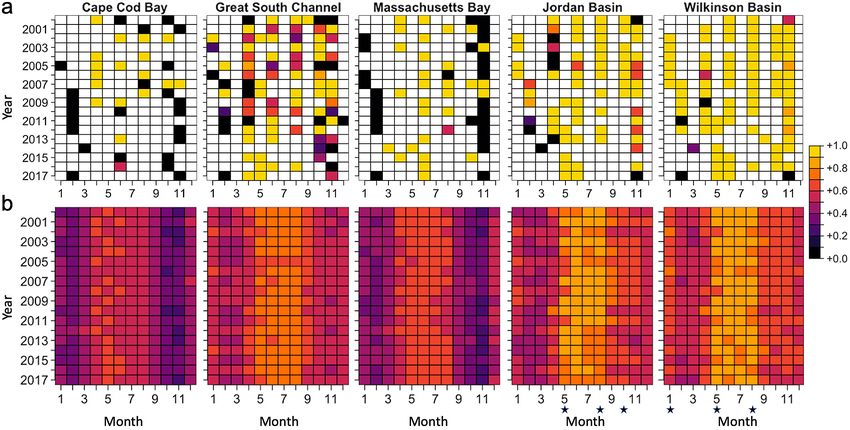
2                                          Mar Ecol Prog Ser 703: 1–16, 2023

et al. 2021). E. glacialis are observed in areas with        coupled biophysical model of the C. finmarchicus life
dense C. finmarchicus aggregations (Wishner et al.           cycle and abundance in the western Gulf of Maine suf-
1988, 1995, Murison & Gaskin 1989, Mayo & Marx               ficiently simulated this species’ phenology for use in a
1990, Kenney & Wishner 1995, Baumgartner & Mate              whale forecast (Pershing et al. 2009a,b). While previous
2003, Baumgartner et al. 2003, Jiang et al. 2007) and        modeling efforts have focused on C. finmarchicus
they appear to select these areas based on whether           abundance, they have not yet characterized the envi-
abundances are above a critical feeding threshold            ronmental conditions associated with the formation of
(Mayo & Marx 1990, Kenney & Wishner 1995). While             high-density aggregations that influence E. glacialis
considerable research has been devoted to under-             foraging behavior. A focus on abundance tends to
standing the abundance and distribution patterns of          smooth out the extreme values that would describe
C. finmarchicus (e.g. Wishner et al. 1988, Kann &            high-density prey patches, as most skill metrics are op-
Wishner 1995, Meise & O’Reilly 1996, Lynch et al.            timized across the full abundance distribution. Gener-
1998, Pershing et al. 2009a, Ji 2011, Reygondeau &           ally, models are on spatial scales that are very coarse
Beaugrand 2011, Record et al. 2013, 2018, Chust et al.       (e.g. Reygondeau & Beaugrand 2011) or use smoothed
2014, Melle et al. 2014, Runge et al. 2015, Ji et al.        approaches, such as generalized additive models
2017, Sorochan et al. 2019), far fewer studies have fo-      (Grieve et al. 2017), that are useful for looking at broad
cused on the distribution of foraging habitat with prey      dynamics, but are not suitable for the extreme high val-
densities above a feeding threshold (e.g. Pendleton et       ues in the C. finmarchicus distribution that form E.
al. 2012, Plourde et al. 2019).                              glacialis feeding habitat. Essentially, it is the right-hand
   The need for predictive skill is evident in ongoing       tail of the prey abundance distribution that matters for
management challenges in both the USA and Canada             this type of foraging strategy, whereas most modeling
(Record et al. 2019, Meyer-Gutbrod et al. 2021). For         approaches focus on the middle of the distribution.
example, sea surface and bottom temperatures in the             Dense aggregations of C. finmarchicus in the North-
Gulf of Maine have been warming rapidly, particu-            west Atlantic form by complex interactions among
larly between 2005 and 2015 (Pershing et al. 2015,           local production, predation, and external supply
Record et al. 2019, Friedland et al. 2020, Gonçalves         (Ji et al. 2022), individual behaviors, and physical
Neto et al. 2021). While species distribution models         oceanographic concentrating mechanisms (Wishner
have estimated a gradual northeastward shift of 8.1          et al. 1988, Epstein & Beardsley 2001, Davies et al.
km per decade in the distribution of C. finmarchicus         2014; reviewed by Sorochan et al. 2021). For most of
(Chust et al. 2014), abrupt shifts occurring within the      the year, the primary prey resource for E. glacialis is
past decade outpace these projections, and distribu-         C. finmarchicus. Additionally, the type of aggrega-
tions have large regional variation (Ji et al. 2022).        tion that E. glacialis may target also depends on the
Changes in the Gulf Stream drove an abrupt shift to          size composition of individual C. finmarchicus. In the
warmer temperatures in the deep waters entering the          Great South Channel, E. glacialis likely target aggre-
Gulf of Maine beginning in 2008 (Gonçalves Neto et           gations of later stage C. finmarchicus, as opposed to
al. 2021), which caused a decline in C. finmarchicus         targeting aggregations based on density alone (Ken-
abundance in the eastern Gulf of Maine by 2010               ney & Wishner 1995). These aggregations can last for
(Record et al. 2019). E. glacialis responded by shifting     several days and cover several square kilometers
from the eastern Gulf of Maine to the Gulf of St.            (Wishner et al. 1988).
Lawrence to forage in summer, resulting in unfore-              Here we analyze C. finmarchicus distribution
seen mortality due to entanglements and ship strikes.        through the lens of E. glacialis foraging behavior on
The resulting shifts in right whale foraging and, con-       the northeastern US continental shelf using the con-
sequently, population growth have put the viability of       cept of a feeding threshold: the prey aggregation
the species in question (Kraus et al. 2016, Davis et al.     density above which foraging becomes energetically
2017). Improved prediction could help management             advantageous for E. glacialis. Local high-density cope-
be more adaptive to such abrupt shifts in foraging           pod aggregations are often described as ‘patches’ or
habitat (Davies & Brillant 2019). Examples of more           ‘swarms,’ although there is no clear agreement on
adaptive management could include directing future           the level of abundance density that delineates one of
survey effort and aiding in longer term planning.            these designations. Similarly, the magnitude of a
   The accuracy of E. glacialis habitat-use models can be    feeding threshold for E. glacialis is not precisely
improved by the inclusion of a prey field (e.g. Pendleton    known, and likely depends on internal factors, such
et al. 2012), highlighting the importance of developing a    as energetic needs and satiation level that vary with
suitable prey field for use as input to these models. A      demographic stage (e.g. Miller et al. 2011, Fortune et
Ross et al.: Estimating right whale prey using thresholds                                 3

al. 2013), as well as external factors, such as prey
species, developmental stage, energy density, verti-
cal distribution, interannual and individual variabil-
ity in lipid content at different developmental stages
(for C. finmarchicus, in particular), and the prey
potentially available elsewhere. We therefore took
an approach where we constrained the problem with
upper and lower bounds on the minimum abundance
of individual C. finmarchicus required to constitute a
high-density patch. We described patches using a
hypothetical right whale feeding density threshold, τ.
Then, we analyzed the sensitivity of the C. fin-
marchicus model output to 4 potential values of τ be-
tween those bounds obtained from the literature (see
Table 2). To avoid confusion around terms such as
‘patchiness,’ we referred to these high-density ag-
gregations as ‘τ-patches.’
   We empirically estimated the presence of C. fin-
marchicus τ-patches in excess of potential E. glaci-
alis feeding thresholds. Based on an extensive liter-
ature review of field studies of feeding E. glacialis, we
examined multiple feeding thresholds in order to clas-         Fig. 1. Study area with critical habitat polygons for Cape
sify the abundances of C. finmarchicus as patch or no-         Cod Bay and the Great South Channel, and potential habi-
patch. We also identified the advantages and tested            tats: Jordan Basin, Massachusetts Bay, and Wilkinson Basin.
the limitations of statistical modeling approaches,            The Massachusetts Bay polygon is superimposed onto the
                                                               Cape Cod Bay polygon due to geographic overlap. black
specifically those of random forest models. The result-
                                                               points indicate the National Oceanic and Atmospheric Ad-
ing modeled prey fields were designed for use as               ministration (NOAA) Fisheries Ecosystem Monitoring Pro-
input to the North Atlantic right whale density surface        gram (MARMAP/EcoMon) survey stations from 2000 to 2017.
model developed for use by the US Navy’s Atlantic              Due to the randomly stratified sampling design, every station
                                                                               was likely only sampled once
Fleet Training and Testing (AFTT) Phase IV Environ-
mental Impact Statement and the National Oceanic
and Atmospheric Administration’s (NOAA’s) Atlantic             Bay, and Wilkinson Basin, which are all important
Large Whale Take Reduction Team (i.e. the Duke                 Calanus finmarchicus sampling locations (Fig. 1)
right whale density surface model version 9: hereafter         (Pendleton et al. 2009). While we highlighted these
‘right whale density model’) (Roberts et al. 2016,             specific regions for visualization and comparison, the
2020) to examine potential management strategies,              model encompassed the domain used in the right
such as targeted closures and reduction of vertical            whale density model.
lines. Beyond the utility of the prey fields, this study
presents a novel approach to modelling and thinking
about copepod data through the lens of predation.                                  2.2. Data sources

                                                                 C. finmarchicus data were obtained from the
          2. MATERIALS AND METHODS                             NOAA Fisheries Ecosystem Monitoring Program
                                                               (MARMAP/EcoMon) survey (https://www.st.nmfs.
                   2.1. Study area                             noaa.gov/copepod/time-series/us-50101/). Briefly,
                                                               samples were collected using a 333 μm mesh bongo
  The study area was the northeastern US continen-             net towed obliquely from the surface to 200 m depth,
tal shelf from the Mid-Atlantic Bight to the eastern           or the bottom in shallower regions (Kane 2007,
Gulf of Maine (Fig. 1). The study area included 2 crit-        Richardson et al. 2010). The mesh size is approxi-
ical habitat regions for Eubalaena glacialis: Cape             mately equivalent to the estimated filtering efficiency
Cod Bay (Mayo et al. 2004) and the Great South                 of E. glacialis baleen (Mayo et al. 2001) and reflects
Channel (CETAP 1982, Kenney & Wishner 1995). We                the size groups with prosome lengths >1.5 mm that
also chose to include Jordan Basin, Massachusetts              would likely be captured by whales (Lehoux et al.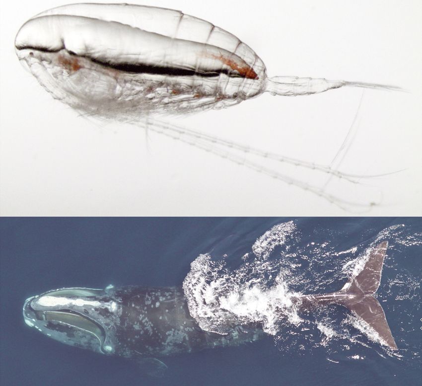
4                                             Mar Ecol Prog Ser 703: 1–16, 2023

2020). We used both the total C. finmarchicus abun-                (Stephens & Krebs 1986), where foragers make deci-
dance (denoted ‘unstaged’ here) captured by the net                sions about whether to stay and feed in a patch or
(predominantly stages C2 through adult), as well as                search for a better patch based on metrics such as
the late stage abundance (C4 through adult). Abun-                 prey density. For E. glacialis foraging, this amounts to
dance data were converted to absence or presence of                exploring different thresholds (τ) of copepod prey
a τ-patch (denoted by zero and one, respectively)                  concentration. Copepods are sampled in a wide vari-
based on whether or not the abundance measured in                  ety of ways, including nets (of various mesh sizes), op-
a sample was below or above the nominal feeding                    tics, acoustics, surface measurements versus water
threshold, τ. Presences/absences of τ-patches were                 column measurements, and at a range of spatial and
then examined for association with a set of environ-               temporal resolutions. The most widespread copepod
mental covariates, including sea surface temperature,              measurements in our region are the water column net
bottom water temperature, sea surface salinity, bot-               tows comprising the EcoMon dataset, reported as in-
tom water salinity, wind, bathymetry, bathymetric                  dividuals (ind.) m−2. Thus, as we estimated upper and
slope, time-integrated surface chlorophyll, sea sur-               lower reasonable and extreme bounds for τ, we con-
face temperature gradient, current speed in the u and              verted to units of ind. m−2 — i.e. what would be sam-
v direction, and day of year (DoY). Monthly environ-               pled by a vertical tow. The challenge is that whales
mental covariates were the same as those used in the               feed on high-density layers within a vertical tow.
right whale density model (Table 1) (Roberts et al.                Suppose a vertical tow measured an ind. m−2 density
2016, 2020). These monthly covariates reflect interan-             of C. finmarchicus, C 2: determining whether this is
nual variability across the time period of this                    above or below a threshold, τ, depends on the propor-
modeling exercise, from 2000 to 2017. The derived                  tion, p, of the profile that is concentrated into a dense
covariates (i.e. time-integrated surface chlorophyll,              layer, and the layer thickness, z. The prey resource
current velocity gradient, sea surface temperature                 available is then C 3 = pC2/z, where the subscripts refer
gradient) were produced from these fields using R                  to density m−3 and m−2, respectively. If we suppose a
(version 4.0.3; R Core Team 2021).                                 layer thickness of z = 20 m, for example, (cf. Baumgart-
                                                                   ner & Mate 2003), and p = 0.7, then a threshold of τ =
                                                                   40 000 ind. m−2, as reported in Record et al. (2019), cor-
                   2.3. Modeling framework                         responds to a feeding layer of 1400 ind. m−3, similar to
                                                                   the values reported by others using these units
  We developed a C. finmarchicus τ-patch formation                 (Table 2) (Murison & Gaskin 1989, Mayo & Marx 1990,
threshold approach to parameterize the model. This                 Woodley & Gaskin 1996, Michaud & Taggart 2007).
approach was derived from optimal foraging theory                  Physical and biological processes can concentrate

Table 1. Monthly mean environmental covariates used in the τ-patch model were obtained from the North Atlantic right whale
density surface model developed for use by the US Navy’s Atlantic Fleet Training and Testing (AFTT) Phase IV Environmental
Impact Statement and the National Oceanic and Atmospheric Administration’s (NOAA’s) Atlantic Large Whale Take Reduc-
tion Team (i.e. the Duke right whale density surface model version 9) (Roberts et al. 2016, 2020). The covariates used are listed
                                    below, along with product and corresponding website

    Covariate(s)                Product                                           More information

    Wind                        Cross-Calibrated Multi-Platform (CCMP) Wind       www.remss.com/measurements/ccmp/
                                 Vector Analysis Product Version 2
    Chlorophyll-a               Copernicus-GlobColour processor                   https://resources.marine.copernicus.eu/
                                                                                   ?option=com_csw&task=results?option=
                                                                                   com_csw&view=details&product_id=
                                                                                   OCEANCOLOUR_GLO_CHL_L4_REP_
                                                                                   OBSERVATIONS_009_082
    Sea surface temperature,    GOFS 3.1 Hybrid Coordinate Ocean Model            https://www.hycom.org/dataserver/gofs-
     Bottom temperature,         (HYCOM) + Navy Coupled Ocean Data                 3pt1/analysis
     Sea surface salinity,      Assimilation (NCODA) Global 1/12° Analysis
     Bottom salinity,            (GLBv0.08)
     Current velocity (u & v)
    Bathymetry, Slope           SRTM30_PLUS bathymetry                            https://topex.ucsd.edu/WWW_html/srtm30
                                                                                   _plus.html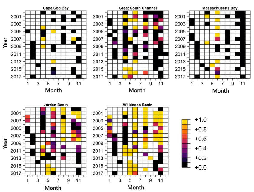
Ross et al.: Estimating right whale prey using thresholds                                              5

Table 2. Literature review for Eubalaena glacialis–Calanus finmarchicus aggregation thresholds. The table includes the liter-
ature source, corresponding C. finmarchicus density with respect to E. glacialis feeding, and any relevant notes about how the
density was obtained. The abundance densities were converted to upper and lower bounds ( p = 1.0 and z = 1 m and 20 m,
respectively) of ind. m−2 measurements based on methods described in Section 2.3; where p represents the proportion of the
                       profile that is concentrated into a dense layer and z represents the layer thickness

 Source                        C. finmarchicus                   Notes                   Location      Lower bound Upper bound
                                    density                                                              (z = 1 m)  (z = 20 m)

 Baumgartner & Mate (2003) Minimum 3600 m−3                 Based on linear           Bay of Fundy,      3600 m−2        72 000 m−2
                                                           regression model           Scotian Shelf
 Baumgartner et al. (2017)    14900 ± 14 400 m−3        Maximum late-stage            Cape Cod Bay,     14 900 m−2       29 8000 m−2
                                                         abundance in upper        Great South Channel,
                                                        15 m of water column        Stellwagen Bank,
                                                                                      Bay of Fundy,
                                                                                     Roseway Basin,
                                                                                      Jeffreys Ledge
 Beardsley et al. (1996)          8.7 × 10³ to         First number is the   Great South Channel         8700 m−2        820 000 m−2
                                 4.1 × 10⁴ m−3      mean for the MOCNESS
                                                   approach. Second number
                                                    is the mean for acoustic
                                                            approach
 Fortune et al. (2013)         6618 ± 3481 m−3                                        Bay of Fundy       6618 m−2        132 360 m−2
 Fortune et al. (2013)        14 778 ± 18 594 m−3                                     Cape Cod Bay      14 778 m−2       295 960 m−2
                                   5           6   −3                                                              −2
 Kenney et al. (1986)        3 × 10 to 1 × 10 m          Minimum to feed on        Great South Channel 300 000 m        20 000 000 m−2
                                                         routinely for survival
 Mayo & Marx (1990)             6.54 × 10³ m−3            Density in regions          Cape Cod Bay       1000 m−2        20 000 m−2
                                   observed                with right whale
                              1000 m−3 suggested              presence
                                 in discussion
 Michaud & Taggart (2007)          900 m−3          Minimum to define right           Bay of Fundy       900 m−2         18 000 m−2
                                                    whale habitat based on
                                                        energy density
 Murison & Gaskin (1989)        832 to 1070 m−3           Minimum to define           Bay of Fundy       832 m−2         21 400 m−2
                                                          right whale habitat.
                                                         First estimate is 1983;
                                                        second estimate is 1984
 Record et al. (2019)             40 000 m−2       Minimum threshold for high          Eastern Gulf     35 000 m−2       45 000 m−2
                                                     right whale occupancy              of Maine
 Wishner et al. (1988)            41 600 m−3          Maximum abundance Great South Channel 41 600 m−2                   832 000 m−2
                                                    from MOCNESS tow near
                                                       feeding right whales
 Wishner et al. (1995)             9749 m−3        Near feeding right whales         Northern Great      9749 m−2        194 980 m−2
                                                                                     South Channel
 Woodley & Gaskin (1996)           1139 m−3         Depth-averaged density            Bay of Fundy       1139 m−2        22 780 m−2

copepods into layers at least as thin as z = 5 m (Mayo                   between the extreme lower bound calculation and the
& Marx 1990). To test the full sensitivity of the model                  threshold density from Record et al. (2019), which re-
to these assumptions, we set p = 1 and z = 1 m and                       sulted in 4 potential density threshold estimates of τ =
20 m. In practice, z is likely >1 m and p < 1, but testing               1000, 4000, 10 000, and 40 000 ind. m−2 (Fig. 2).
the more extreme values (i.e. z = 1 m) gives a fuller                      Models were trained on the EcoMon dataset. Ran-
understanding of the model behavior. We used these                       dom forest models were built using the biomod2
unlikely, extreme values only to compute the lower                       package in R using 10 cross-validation folds with ran-
bound of the potential τ estimates suggested in the lit-                 dom 70% to 30% training to testing data splits
erature (i.e. τ = 1000 ind. m−2) (Mayo & Marx 1990).                     (Thuiller et al. 2009, R Core Team 2021). Random
We then used these assumptions along with the litera-                    forests are highly accurate predictive models (Li &
ture review in Table 2 to select 2 intermediate values                   Wang, 2013) that can be configured for either classifi-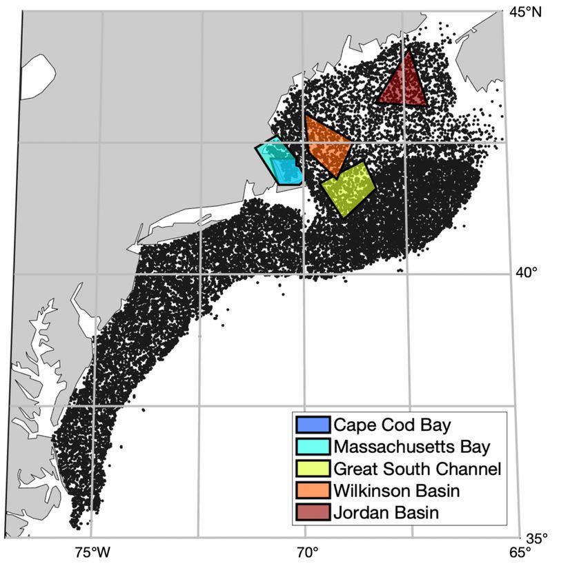
6                                              Mar Ecol Prog Ser 703: 1–16, 2023

                                                                                     both with the entire dataset (using
                                                                                     DoY as a covariate; hereafter referred
                                                                                     to as the ‘whole-year’ method), and as
                                                                                     12 individual monthly climatological
                                                                                     models. Running the model with 4
                                                                                     thresholds, 2 stage delineations, and
                                                                                     whole-year and monthly methods pro-
                                                                                     duced 16 final random forest models.
                                                                                     We also ran ensembles of generalized
                                                                                     additive models, boosted regression
                                                                                     trees, and random forest models, for a
                                                                                     total of 48 model configurations
                                                                                     (Fig. 3). Here, we present the highest
                                                                                     performing configuration, based on
                                                                                     AUC, with the most plausible habitat
Fig. 2. Abundance of Calanus finmarchicus (log10 ind. m−2) from 2000 to 2017         maps — the random forest model, using
for the unstaged National Oceanic and Atmospheric Administration (NOAA)              the unstaged data sampled with a
Fisheries Ecosystem Monitoring Program (MARMAP/EcoMon) dataset. Gray                 mesh size theoretically equivalent to
vertical lines indicate the 4 different τ-patch formation thresholds used in this    the filtering efficiency of right whale
study (τ = 1000, 4000, 10 000, and 40 000 ind. m−2, respectively). Horizontal bars
show Eubalaena glacialis feeding thresholds surveyed in the literature review
                                                                                     baleen (Mayo et al. 2001), and using
(see Table 2). The ‘Gulf of Maine’ locations include various sites reported in       DoY as a covariate (i.e. whole-year
         Baumgartner et al. (2017) and Record et al. (2019) (see Table 2)            method).

cation (i.e. this study) or regression problems. The
model consists of a series of decision trees and boot-                                    3. RESULTS
straps data to avoid convergence issues associated
with similar techniques (e.g. classification and re-                   The unstaged EcoMon data comprised a total of
gression trees) (Breiman 2001, Evans et al. 2011).                  8729 Calanus finmarchicus abundance observations,
Area under the receiver operating characteristic                    with a mode around 10 000 ind. m−2. Only a few ob-
curve (AUC) and the true skill statistic (TSS) were                 servations exceeded τ = 1 000 000 ind. m−2 (n = 3;
computed for the random forests using inbuilt bio-                  Fig. 2). Just over one-third of the observations ex-
mod2 functions and were used to evaluate model per-                 ceeded τ = 10 000 ind. m−2 (n = 3280, 37.6% of the
formance. Both metrics are methods commonly used                    total; Fig. 2). Fewer than one-quarter of the observa-
to evaluate species distribution models (Fielding &                 tions exceeded τ = 40 000 ind. m−2 (n = 1276, 14.6% of
Bell 1997, Allouche et al. 2006, Liu et al. 2011, Ross et           the total; Fig. 2). Feeding threshold values (τ) esti-
al. 2021). AUC and TSS both examine a given model’s                 mated from the literature spanned the upper portion
classification performance using the proportion of                  of the distribution with some regional clustering;
true positives. AUC is computed on a scale from 0 to 1,             estimates from Cape Cod Bay and the Bay of Fundy
where a value above 0.5 indicates better performance                were lower than in the Great South Channel (Fig. 2).
than a random model (Fielding & Bell 1997). TSS is                  The highest estimated upper-bound threshold from
computed on a scale of -1 to 1, where a value of 0 indi-            the literature (20 000 000 m−2, estimated from Kenney
cates better performance than a random model (Al-                   et al. 1986; Table 2) exceeded the upper bound rep-
louche et al. 2006). Interannual trends were computed               resented in the EcoMon dataset.
across the model results in the 5 regional polygons                    Qualitative examination of the presence and ab-
(Fig. 1). A linear regression was performed for each                sence of τ-patches in the EcoMon data showed a clear
month to assess interdecadal trends in t-patches over               spatial pattern and seasonality, as well as significant
the study period. Environmental covariates were                     data gaps (Fig. 4). For example, for a threshold of τ =
screened to prevent collinearity in the models. For ex-             10 000 ind. m−2, the presence of τ-patches appeared
ample, if 2 covariates were highly correlated (r > 0.8)             qualitatively to reach a minimum in February, fol-
then the covariate known to have a mechanistic link                 lowed by an increase in the Gulf of Maine and along
with C. finmarchicus aggregation was retained                       the continental slope through the spring and summer,
during the model selection process (e.g. Russo et al.               with the exception of coastal areas. There was a con-
2015, Bosso et al. 2018). We ran random forest models               traction into the deeper basins of the Gulf of Maine in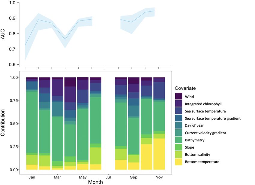
Ross et al.: Estimating right whale prey using thresholds 7
Fig. 3. Modeling decisions considered in this study. The dark blue boxes and arrows highlight the configuration presented with
the unstaged dataset, covariates selected based on correlation analysis, the random forest algorithm, and τ = 10 000 ind. m−2
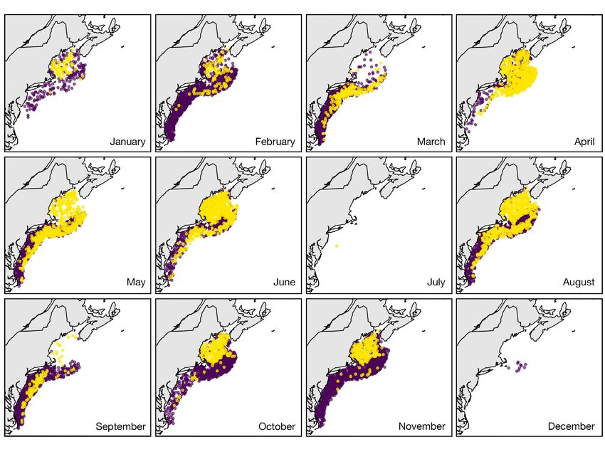
Fig. 4. Monthly presence (yellow points) or absence (purple points) of τ-patches from 2000 to 2017 for a threshold of τ = 10 000
m−2 using the unstaged National Oceanic and Atmospheric Administration (NOAA) Fisheries Ecosystem Monitoring Program
(MARMAP/EcoMon)
late summer and fall and a decline in the winter. Modeled τ-patch distribution and dynamics matched
There was also high τ-patch occurrence along the the seasonal and spatial patterns in the presence/
continental shelf break. The data gap in July and absence of τ-patches in the raw data, which were
December, as well as in the Gulf of Maine for March described in the previous paragraph (Fig. 5). Of the
and September, highlighted the need for models. various model configurations tested, the unstaged
8                                            Mar Ecol Prog Ser 703: 1–16, 2023

Fig. 5. Projections of Calanus finmarchicus τ-patches using thresholds of (a) τ = 10 000 ind. m−2 and (b) τ = 40 000 ind. m−2
for the unstaged National Oceanic and Atmospheric Administration (NOAA) Fisheries Ecosystem Monitoring Program
                                               (MARMAP/EcoMon) dataset
Ross et al.: Estimating right whale prey using thresholds                                  9

Table 3. Model performance for 4 versions of the random            ferred to as prey ‘patchiness’. This variability is par-
forest model evaluated using area under the receiver oper-         ticularly pronounced for the τ = 40 000 ind. m−2 model
ating characteristic curve (AUC) and the true skill statistic
                                                                   (Fig. 5b). EcoMon data do not extend off the conti-
(TSS). AUC is computed on a 0 to 1 scale (± SE). TSS is com-
puted on a −1 to 1 scale (± SE). With both metrics, a higher       nental shelf, so it is difficult to validate the model
         score indicates better model performance                  extrapolation into this habitat. However, the moder-
                                                                   ate values off the shelf in some months are probably
 Model version                  AUC               TSS              unrealistic, as this is generally not C. finmarchicus
                                                                   habitat.
 1000 ind. m−2 unstaged     0.915 ± 0.00141 0.6737 ± 0.00304          The gaps in the EcoMon data make it difficult to
 4000 ind. m−2 unstaged     0.919 ± 0.00126 0.6887 ± 0.00353
                                                                   determine trends in τ-patches over time (Fig. 6a).
 10 000 ind. m−2 unstaged   0.925 ± 0.00187 0.705 ± 0.00414
 40 000 ind. m−2 unstaged   0.907 ± 0.00171 0.682 ± 0.00355        Modeled τ-patch fields allowed us to interpolate these
                                                                   data gaps, giving one way to estimate whether feed-
                                                                   ing habitats are becoming better or worse over time.
data with a threshold of τ = 10 000 ind. m−2 using the             We computed trends for each month at each of the 5
whole-year method performed the best based on                      E. glacialis habitats outlined in Fig. 1 (i.e. Cape Cod
both metrics (Table 3), so most of the results shown               Bay, Massachusetts Bay, the Great South Channel,
will focus on that configuration. The threshold of τ =             Jordan Basin, and Wilkinson Basin). Trends were sig-
40 000 ind. m−2 also performed well and is included                nificant in certain months using the τ = 10 000 ind. m−2
in e.g. Fig. 5b. In both models, there is a seasonal               threshold model in the deep basins of the Gulf of
minimum in February, an increase through the                       Maine (i.e. Jordan Basin and Wilkinson Basin; Fig. 6b).
spring and summer, and a contraction into the deep                 In May, the trends were positive, indicating an in-
basins in the fall (Fig. 5). In contrast to models of C.           crease from 2000 to 2017 in Jordan Basin (r = 0.704,
finmarchicus abundance, the spatial distributions                  p = 0.00111) and Wilkinson Basin (r = 0.772, p < 0.001).
have a high degree of variability that follows bathy-              In August, the trends were negative in Jordan Basin
metric and oceanographic features; this is often re-               (r = −0.648, p = 0.00364) and Wilkinson Basin (r =

Fig. 6. (a) Plots of the proportion of abundances that exceeded a threshold value of τ = 10 000 ind. m−2 for the unstaged
National Oceanic and Atmospheric Administration (NOAA) Fisheries Ecosystem Monitoring Program (MARMAP/EcoMon)
data. (b) Plots of the prediction of patch formation from the random forest model for a threshold value of τ = 10 000 ind. m−2 on
          a 0 to 1 scale. A star under the x-axis label indicates trends for that month were significant in a given region
10 Mar Ecol Prog Ser 703: 1–16, 2023
−0.657, p = 0.00303). In October, the trend was nega- probabilities. The strongest correlation was for τ =
tive in Jordan Basin (r = −0.733, p = 0.000543). Trends 10 000 ind. m−2.
were similar for the τ = 40000 ind. m−2 in the deep Monthly model runs allowed us to tease apart the
basins in May and August, as well. Positive trends covariate contributions to the model and model per-
were found in May and negative trends were found formance by time of year. Covariate contributions
in August in the deep basins. In October, the trend varied seasonally, but bathymetry was consistently
was negative in Wilkinson Basin (r = −0.607, p = the strongest contributor (Fig. 8). From late summer
0.00754). No significant trends were found in Cape through winter, bottom oceanography had a large
Cod Bay, Massachusetts Bay, or the Great South contribution. The combined effects of deep-water
Channel. properties (i.e. bottom temperature and salinity) was
Modeled τ-patch likelihoods matched measured a strong contributor in the late summer and fall, con-
frequencies well, with some notable differences sistently stronger than sea surface temperature dur-
depending on the value of τ. Comparing models and ing this period. In winter months, bottom salinity
data requires some data binning so that both values was the second strongest contributor (behind bathy-
fall along a continuous scale from 0 to 1. For compar- metry). By contrast, the contribution by surface pro-
ison, we binned both by month and year, resulting in cesses (sea surface temperature, surface temperature
scatter plots with 216 points (Fig. 7). There were cor- gradient, wind, time-integrated surface chlorophyll,
relations for every selected value of τ. Modeled val- and current velocity gradient) peaked in March and
ues tended to overestimate for low probabilities of a April. Time-integrated surface chlorophyll was the
τ-patch and match the one-to-one line better for high second strongest predictor (behind bathymetry) in
these months. The seasonal shift between contribu-
tions by surface versus bottom covariates aligned
with the seasonal life history strategy of C. finmarchi-
cus, with deep-water diapause in late summer
through winter, and emergence and reproduction
following from the spring phytoplankton bloom. The
monthly models were unable to run in July and
December due to data gaps as a result of under-
sampling. Model performance varied seasonally, as
well, with AUC generally exceeding a value of 0.8
throughout the year.
Focusing again on the whole-year τ = 10 000 ind.
m−2 model, response curves generally showed uni-
modal responses across all covariates (Fig. 9). The
strong seasonality was reflected in the modeled
response to the DoY covariate, which helped to inter-
polate across the data gaps in July and December.
For most covariates, the full scope of the model falls
within the well-sampled range of data, with the
exception of bathymetry. High bathymetry regions
(i.e. deep, off-shelf waters) were undersampled,
leading to model extrapolation that was probably
unrealistically high where the sample representation
dropped off. Model cross-validation runs matched
each other closely, particularly where sampling was
Fig. 7. Measured probability of a high-density τ-patch ver-
high.
sus the modeled probability of a τ-patch for (a) τ = 1000 ind.
m−2 (r2 = 0.49), (b) τ = 4000 ind. m−2 (r2 = 0.58), (c) τ = 10 000
ind. m−2 (r2 = 0.63), and (d) τ = 40 000 ind. m−2 (r2 = 0.49) for
the unstaged National Oceanic and Atmospheric Adminis- 4. DISCUSSION
tration (NOAA) Fisheries Ecosystem Monitoring Program
(MARMAP/EcoMon) dataset at a significance level of p <
0.001. Points were averaged spatially, with one data point Management of Eubalaena glacialis could likely be
per month per year (n = 216). The black line shows the improved by the incorporation of prey information
theoretical one-to-one line into models and decision support tools (Pendleton etRoss et al.: Estimating right whale prey using thresholds 11
Fig. 8. Monthly covariate contributions with the corresponding model evaluations shown in the top panel. Shaded regions indi-
cate the minimum and maximum area under the receiver operating characteristic curve (AUC) values of the 10 cross-validation
runs for a given month
al. 2012, Brennan et al. 2021, Ross et al. 2021). How- annual, and possibly regional variability. Under-
ever, there is a disconnect between knowledge of standing how τ varies depending on changing condi-
Calanus finmarchicus population dynamics and the tions represents an important next step in the predic-
need for finer-scale information on the high-density tion of E. glacialis movements.
copepod aggregations that E. glacialis requires. At a high level, τ-patch dynamics, particularly
Models and analysis do not generally capture the those at the τ = 10 000 ind. m−2 and 40 000 ind. m−2
high-abundance end of the C. finmarchicus distribu- levels, followed documented patterns in E. glacialis
tion, which does not necessarily track with overall movements during the times of year when whales
abundance patterns because of oceanographic and feed on C. finmarchicus. The absence of late summer
biological processes operating at different spatial C. finmarchicus abundances exceeding 40 000 m−2 in
and temporal scales. Jordan Basin after 2010, for example, matched the
We modeled the spatiotemporal patterns of τ- timing of the decline of E. glacialis use of the eastern
patches to better understand their dynamics and Gulf of Maine as a foraging ground (Fig. A1 in the
develop products for incorporating these dynamics Appendix) (Record et al. 2019). One notable feature
into decision support tools. This required exploring a of the τ-patch model is that there is finer scale spatial
threshold value, τ, that defined a prey density high variability than with C. finmarchicus abundance
enough to attract E. glacialis feeding. Empirical criti- models, which are generally much smoother in space
cal feeding thresholds reported in the literature vary (e.g. Pershing et al. 2009a, Reygondeau & Beaugrand
widely (Table 2), which is not surprising because of 2011, Grieve et al. 2017). This could provide added
the many factors that could influence foraging deci- information for predicting foraging decisions made
sions. A full picture of τ would show monthly, inter- by E. glacialis. Certain features were picked up by12 Mar Ecol Prog Ser 703: 1–16, 2023
Fig. 9. Response curves for the model with a threshold of τ = 10 000 ind. m−2 with the unstaged National Oceanic and Atmos-
pheric Administration (NOAA) Fisheries Ecosystem Monitoring Program (MARMAP/EcoMon) data. Each line represents one
of 10 cross-validation foldsRoss et al.: Estimating right whale prey using thresholds 13 the τ-patch models, such as the higher values along tidal fronts, although models are improving (e.g. the edge of the continental shelf; this feature appears Brennan et al. 2019). Nevertheless, the statistical dis- in the EcoMon data but is not captured by smoother tribution of in situ samples of copepods does capture abundance models. This patchy spatial pattern is the occurrence of dense aggregations. Random more pronounced the further toward the high end of forests are highly accurate predictive species distri- the distribution τ is, especially at τ = 40 000 ind. m−2. bution models (Li & Wang, 2013), and they are able to It is an encouraging indication that modeling τ- accurately predict the probability of C. finmarchicus patches could be a helpful approach to understand τ-patches at the scales examined. Linking the empiri- the foraging patterns of E. glacialis. cal associations of τ-patches with ultra-fine-scale There are some notable differences between the τ- mechanistic models represents an important area of patches and C. finmarchicus abundance in covariate future work that could improve maps of E. glacialis associations when comparing with previous statistical prey distribution. Key next steps include coupling to models. For example, the favorable sea surface tem- vertically resolved data and models (Plourde et al. perature range of C. finmarchicus statistically esti- 2019, Brennan et al. 2021) and linking models across mated by published models has ranged from 4.5− the full international domain of E. glacialis foraging. 8.5°C (Reygondeau & Beaugrand 2011) to 6−10°C The ultimate goal of this work was to provide prey (Helaouët & Beaugrand 2007). In contrast, the highest information that could be used in decision support τ-patch probabilities in our model occurred for sea tools for E. glacialis management. The next step is to surface temperatures of 7−15°C (Fig. 9). Similarly, link these modeled prey fields to the right whale modeled estimates using bottom temperatures have modeling used to support decision making (Roberts found peaks at
14                                             Mar Ecol Prog Ser 703: 1–16, 2023

into decision support promise to be helpful. A closer                 tal shelf. Final report, contract no. AA551-CT8−48,
look at the dynamics of the highest-density aggrega-                  Bureau of Land Management, Washington, DC
                                                                  Chust G, Castellani C, Licandro P, Ibiabarriaga L, Sagarmi-
tions of prey gives a new lens to an old problem and                  naga Y, Irigoien X (2014) Are Calanus spp. shifting pole-
could provide another tool for helping to predict right               ward in the North Atlantic? A habitat modelling ap-
whale movements.                                                      proach. ICES J Mar Sci 71:241−253
                                                                  Cooke JG (2020) Eubalaena glacialis (errata version pub-
                                                                      lished in 2020). IUCN Red List Threat Anim 2020:
Data availability. The computed τ-patch fields are available          e.T41712A178589687
from the corresponding author (C. H. Ross) upon request.          Davies KTA, Brillant SW (2019) Mass human-caused mortal-
                                                                      ity spurs federal action to protect endangered North
                                                                      Atlantic right whales in Canada. Mar Policy 104:157−162
Acknowledgements. We thank those who participated in              Davies KTA, Taggart CT, Smedbol RK (2014) Water mass
collecting the National Oceanic and Atmospheric Adminis-              structure defines the diapausing copepod distribution in
tration (NOAA) Fisheries Ecosystem Monitoring Program                 a right whale habitat on the Scotian Shelf. Mar Ecol Prog
(MARMAP/EcoMon) data and Harvey Walsh for providing                   Ser 497:69−85
updated data and species stage information. We thank              Davis GE, Baumgartner MF, Bonnell JM, Bell J and
Daniel E. Pendleton, Kimberly T. A. Davies, and 3 anony-              others (2017) Long-term passive acoustic recordings
mous reviewers for their feedback on this manuscript. This            track the changing distribution of North Atlantic right
work was funded by NOAA grant NA20NMF0080246, MBON                    whales (Eubalaena glacialis) from 2004 to 2014. Sci
grant NA19NOS0120197, BOEM Cooperative Agreement                      Rep 7:13460
M19AC00022, the Maine Community Foundation, Tandy                 Epstein AW, Beardsley RC (2001) Flow-induced aggregation
Center for Ocean Forecasting institutional funds, and                 of plankton at a front: a 2-D Eulerian model study. Deep
Bigelow Laboratory for Ocean Sciences institutional funds.            Sea Res II 48:395−418
                                                                  Evans JS, Murphy MA, Holden ZA, Cushman SA (2011) Mod-
                                                                      eling species distribution and change using random forest.
                    LITERATURE CITED                                  In: Drew CA, Wiersma YF, Huettmann F (eds) Predictive
                                                                      species and habitat modeling in landscape ecology: con-
Allouche O, Tsoar A, Kadmon R (2006) Assessing the accu-              cepts and applications. Springer, New York, NY, p 139−159
   racy of species distribution models: prevalence, kappa,        Fielding AH, Bell JF (1997) A review of methods for the
   and the true skill statistic (TSS). J Appl Ecol 43:1223−1232       assessment of prediction errors in conservation presence/
Baumgartner MF, Mate BR (2003) Summertime foraging                    absence models. Environ Conserv 24:38−49
   ecology of North Atlantic right whales. Mar Ecol Prog          Fortune SME, Trites AW, Mayo CA, Rosen DAS, Hamilton
   Ser 264:123−135                                                    PK (2013) Energetic requirements of North Atlantic right
Baumgartner MF, Cole TVN, Clapham PJ, Mate BR (2003)                  whales and the implications for species recovery. Mar
   North Atlantic right whale habitat in the lower Bay of             Ecol Prog Ser 478:253−272
   Fundy on the SW Scotian Shelf during 1999−2001. Mar            Friedland KD, Morse RE, Manning JP, Melrose DC and oth-
   Ecol Prog Ser 264:137−154                                          ers (2020) Trends and change points in surface and bot-
Baumgartner MF, Wenzel FW, Lysiak NSJ, Patrician MR                   tom thermal environments of the US Northeast Conti-
   (2017) North Atlantic right whale foraging ecology and             nental Shelf Ecosystem. Fish Oceanogr 29:396−414
   its role in human-caused mortality. Mar Ecol Prog Ser          Gonçalves Neto A, Langan JA, Palter JB (2021) Changes in
   581:165−181                                                        the Gulf Stream preceded rapid warming of the North-
Beardsley RC, Epstein AW, Chen CS, Wishner KF, Macaulay               west Atlantic Shelf. Nat Commun Earth Environ 2:74
   MC, Kenney RD (1996) Spatial variability in zooplankton        Grieve BD, Hare JA, Saba VS (2017) Projecting the effects of
   abundance near feeding right whales in the Great South             climate change on Calanus finmarchicus distribution
   Channel. Deep Sea Res II 43:1601−1625                              within the U.S. Northeast Continental Shelf. Sci Rep 7:
Bosso L, Smeraldo S, Rapuzzi P, Sama G, Garonna AP, Russo             6264
   D (2018) Nature protection areas of Europe are insuffi-        Helaouët P, Beaugrand G (2007) Macroecology of Calanus
   cient to preserve the threatened beetle Rosalia alpina             finmarchicus and C. helgolandicus in the North Atlantic
   (Coleoptera: Cerambycidae): evidence from species dis-             Ocean and adjacent seas. Mar Ecol Prog Ser 345:147−165
   tribution models and conservation gap analysis. Ecol           Ji R (2011) Calanus finmarchicus diapause initiation: new
   Entomol 43:192−203                                                 view from traditional life history-based model. Mar Ecol
Breiman L (2001) Random forests. Mach Learn 45:5−32                   Prog Ser 440:105−111
Brennan CE, Maps F, Gentleman WC, Plourde S and others            Ji R, Feng Z, Jones BT, Thompson C, Chen C, Record NR,
   (2019) How transport shapes copepod distributions in               Runge JA (2017) Coastal amplification of supply and
   relation to whale feeding habitat: demonstration of a              transport (CAST): a new hypothesis about the persist-
   new modelling framework. Prog Oceanogr 171:1−21                    ence of Calanus finmarchicus in the Gulf of Maine. ICES
Brennan CE, Maps F, Gentleman WC, Lavoie D, Chassé J,                 J Mar Sci 74:1865−1874
   Plourde S, Johnson CL (2021) Ocean circulation changes         Ji R, Runge JA, Davis CS, Wiebe PH (2022) Drivers of vari-
   drive shifts in Calanus abundance in North Atlantic right          ability of Calanus finmarchicus in the Gulf of Maine:
   whale foraging habitat: a model comparison of cool and             roles of internal production and external exchange. ICES
   warm year scenarios. Prog Oceanogr 197:102629                      J Mar Sci 79:775−784
CETAP (Cetacean and Turtle Assessment Program) (1982) A           Jiang M, Brown MW, Turner JT, Kenney RD, Mayo CA,
   characterization of marine mammals and turtles in the              Zhang Z, Zhou M (2007) Springtime transport and reten-
   mid-and North Atlantic areas of the U.S. outer continen-           tion of Calanus finmarchicus in Massachusetts and Cape
Ross et al.: Estimating right whale prey using thresholds 15
Cod Bays, USA, and implications for right whale forag- Pendleton DE, Pershing AJ, Brown MW, Mayo CA, Kenney
ing. Mar Ecol Prog Ser 349:183−197 RD, Record NR, Cole TVN (2009) Regional-scale mean
Kane J (2007) Zooplankton abundance trends on Georges copepod concentration indicates relative abundance of
Bank, 1977−2004. ICES J Mar Sci 64:909−919 North Atlantic right whales. Mar Ecol Prog Ser 378:
Kann LM, Wishner K (1995) Spatial and temporal patterns of 211−225
zooplankton on baleen whale feeding grounds in the Pendleton DE, Sullivan PJ, Brown MW, Cole TVN and oth-
southern Gulf of Maine. J Plankton Res 17:235−262 ers (2012) Weekly predictions of North Atlantic right
Kenney RD, Wishner KF (1995) The South Channel Ocean whale Eubalaena glacialis habitat reveal influence of
Productivity EXperiment. Cont Shelf Res 15:373−384 prey abundance and seasonality of habitat preferences.
Kenney RD, Hyman MAM, Owen RE, Scott GP, Winn HE Endang Species Res 18:147−161
(1986) Estimation of prey densities required by western Pershing AJ, Stamieszkin K (2020) The North Atlantic eco-
North Atlantic right whales. Mar Mamm Sci 2:1−13 system, from plankton to whales. Annu Rev Mar Sci 12:
Kraus SD, Kenney RD, Mayo CA, McLellan WA, Moore MJ, 339−359
Nowacek DP (2016) Recent scientific publications cast Pershing AJ, Record NR, Monger BC, Pendleton DE, Wood-
doubt on North Atlantic right whale future. Front Mar ard LA (2009a) Model-based estimates of Calanus finmar-
Sci 3:137 chicus abundance in the Gulf of Maine. Mar Ecol Prog Ser
Lehoux C, Plourde S, Lesage V (2020) Significance of domi- 378:227−243
nant zooplankton species to the North Atlantic right Pershing AJ, Record NR, Monger BC, Mayo CA and others
whale potential foraging habitats in the Gulf of St. (2009b) Model-based estimates of right whale habitat
Lawrence: a bio-energetic approach. DFO Canadian Sci- use in the Gulf of Maine. Mar Ecol Prog Ser 378:245−257
ence Advisory Secretariat Research Document, 2020/033 Pershing AJ, Hernandez CM, Kerr LA, LeBris A and others
Li X, Wang Y (2013) Applying various algorithms for species (2015) Slow adaptation in the face of rapid warming
distribution modeling. Integr Zool 8:124−135 leads to the collapse of an iconic fishery. Science 350:
Liu C, White M, Newell G (2011) Measuring and comparing 809−812
the accuracy of species distribution models with pres- Plourde S, Lehoux C, Johnson CL, Perrin G, Lesage V (2019)
ence-absence data. Ecography 34:232−243 North Atlantic right whale (Eubalaena glacialis) and its
Lynch DR, Gentleman WC, McGillicuddy DJ Jr, Davis CS food: (I) a spatial climatology of Calanus biomass and
(1998) Biological/physical simulations of Calanus fin- potential foraging habitats in Canadian waters. J Plank-
marchicus population dynamics in the Gulf of Maine. ton Res 41:667−685
Mar Ecol Prog Ser 169:189−210 R Core Team (2021) R: a language and environment for statis-
Mayo CA, Marx MK (1990) Surface foraging behaviour of tical computing. R Foundation for Statistical Computing,
the North Atlantic right whale, Eubalaena glacialis, and Vienna. www.r-project.org
associated zooplankton characteristics. Can J Zool 68: Record NR, Pershing AJ, Maps F (2013) Emergent copepod
2214−2220 communities in an adaptive trait-structured model. Ecol
Mayo CA, Letcher BH, Scott S (2001) Zooplankton filtering Model 260:11−24
efficiency of the baleen of a North Atlantic right whale, Record NR, Ji R, Maps F, Varpe Ø, Runge JA, Petrik CM,
Eubalaena glacialis. J Cetacean Res Manag 3:245−250 Johns DA (2018) Copepod diapause and the biogeogra-
Mayo CA, Nichols OC, Bessinger MK, Brown MW, Marx MK, phy of the marine lipidscape. J Biogeogr 45:2238−2251
Browning CL (2004) Surveillance, monitoring and man- Record NR, Runge JA, Pendleton DE, Balch WM and others
agement of North Atlantic right whales in Cape Cod Bay (2019) Rapid climate-driven circulation changes threaten
and adjacent waters — 2004. Final report submitted to the conservation of endangered North Atlantic right whales.
Commonwealth of Massachusetts, Division of Marine Oceanography 32(2):162−169
Fisheries, Boston, MA Reygondeau G, Beaugrand G (2011) Future climate-driven
Meise CJ, O’Reilly JE (1996) Spatial and seasonal patterns shifts in distribution of Calanus finmarchicus. Glob
in abundance and age composition of Calanus finmar- Change Biol 17:756−766
chicus in the Gulf of Maine and on Georges Bank 1977− Richardson DE, Hare JA, Overholtz WJ, Johnson DL (2010)
1987. Deep Sea Res II 43:1473−1501 Development of long-term larval indices for Atlantic her-
Melle W, Runge J, Head E, Plourde S and others (2014) The ring (Clupea harengus) on the northeast US continental
North Atlantic Ocean as habitat for Calanus finmarchi- shelf. ICES J Mar Sci 67:617−627
cus: Environmental factors and life history traits. Prog Roberts JJ, Best B, Mannocci L, Fujioka E and others (2016)
Oceanogr 129:244−284 Habitat-based cetacean density models for the U.S.
Meyer-Gutbrod EL, Greene CH, Davies KTA, Johns DG Atlantic and Gulf of Mexico. Sci Rep 6:22615
(2021) Ocean regime shift is driving collapse of the North Roberts JJ, Schick RS, Halpin PN (2020) Final Project Report:
Atlantic right whale population. Oceanogr Mag 34:22−31 Marine Species Density Data Gap Assessments and
Michaud J, Taggart CT (2007) Lipid and gross energy content Update for the AFTT Study Area, 2018-2020 (Option Year
of North Atlantic right whale food, Calanus finmarchicus, 3). Document version 1.4. Report prepared for Naval
in the Bay of Fundy. Endang Species Res 3:77−94 Facilities Engineering Command, Atlantic by the Duke
Miller CA, Reeb D, Best PB, Knowlton AR, Brown MW, University Marine Geospatial Ecology Lab, Durham, NC
Moore MJ (2011) Blubber thickness in right whales Ross CH, Pendleton DE, Tupper B, Brickman D, Zani MA,
Eubalaena glacialis and Eubalaena australis related with Mayo CA, Record NR (2021) Projecting regions of Norht
reproduction, life history status and prey abundance. Atlantic right whale, Eubalaena glacialis, habitat suit-
Mar Ecol Prog Ser 438:267−283 ability in the Gulf of Maine for the year 2050. Elem Sci
Murison LD, Gaskin DE (1989) The distribution of right Anthropocene 9:00058
whales and zooplankton in the Bay of Fundy, Canada. Runge JA, Ji R, Thompson CRS, Record NR and others (2015)
Can J Zool 67:1411−1420 Persistence of Calanus finmarchicus in the western Gulf16 Mar Ecol Prog Ser 703: 1–16, 2023
of Maine during recent extreme warming. J Plankton Res Stephens DW, Krebs JR (1986) Foraging theory. Princeton
37:221−232 University Press, Princeton, NJ
Russo D, Di Febbraro M, Cistrone L, Jones G, Smeraldo Thuiller W, Lafourcade B, Engler R, Araújo MB (2009) BIO-
S, Garonna A, Bosso L (2015) Protecting one, protect- MOD — A platform for ensemble forecasting of species
ing both? Scale-dependent ecological differences in distributions. Ecography 32:369−373
two species using dead trees, the rosalia longicorn Wishner K, Durbin E, Durbin A, Macaulay M, Winn H, Ken-
beetle and the barbastelle bat. J Zool (Lond) 297: ney R (1988) Copepod patches and right whales in the
165−175 Great South Channel off New England. Bull Mar Sci 43:
Sorochan KA, Ploudre S, Morse R, Pepin P, Runge JA, 825−844
Thompson C, Johnson CL (2019) North Atlantic right Wishner KF, Schoenherr JR, Beardsley R, Chen C (1995)
whales (Eubalaena glacialis) and its food: (II) interannual Abundance, distribution and population structure of the
variations in biomass of Calanus spp. on western North copepod Calanus finmarchicus in a springtime right
Atlantic shelves. J Plankton Res 41:687−708 whale feeding area in the southwestern Gulf of Maine.
Sorochan KA, Brennan CE, Plourde S, Johnson CL (2021) Cont Shelf Res 15:475−507
Spatial variation and transport of abundant copepod taxa Woodley TH, Gaskin DE (1996) Environmental characteris-
in the southern Gulf of St. Lawrence in autumn. J Plank- tics of North Atlantic right and fin whale habitat in the
ton Res 43:908−926 lower Bay of Fundy, Canada. Can J Zool 74:75−84
Appendix.
Fig. A1. Plots of the proportion of abundances that exceeded a threshold value of τ = 40 000 ind. m−2 for the unstaged National
Oceanic and Atmospheric Administration (NOAA) Fisheries Ecosystem Monitoring Program (MARMAP/EcoMon) data
Editorial responsibility: Sigrun Jónasdóttir, Submitted: April 26, 2022
Charlottenlund, Denmark Accepted: October 28, 2022
Reviewed by: 3 anonymous referees Proofs received from author(s): January 10, 2023You can also read