Glacier geometry and flow speed determine how Arctic marine-terminating glaciers respond to lubricated beds
←
→
Page content transcription
If your browser does not render page correctly, please read the page content below
The Cryosphere, 16, 1431–1445, 2022
https://doi.org/10.5194/tc-16-1431-2022
© Author(s) 2022. This work is distributed under
the Creative Commons Attribution 4.0 License.

Glacier geometry and flow speed determine how Arctic
marine-terminating glaciers respond to lubricated beds
Whyjay Zheng1,2
1 Department   of Earth and Atmospheric Sciences, Cornell University, Ithaca, NY, USA
2 Department   of Statistics, University of California Berkeley, Berkeley, CA, USA

Correspondence: Whyjay Zheng (whyjz@berkeley.edu)

Received: 4 November 2021 – Discussion started: 10 November 2021
Revised: 24 February 2022 – Accepted: 17 March 2022 – Published: 21 April 2022

Abstract. Basal conditions directly control the glacier slid-    the Greenland ice sheet (GrIS), the dynamic discharge of
ing rate and the dynamic discharge of ice. Recent glacier        marine-terminating glaciers accounts for 66 % of the region’s
destabilization events indicate that some marine-terminating     total mass loss (Mouginot et al., 2019). For the other Arc-
glaciers quickly respond to lubricated beds with increased       tic regions outside of the GrIS, surface mass balance con-
flow speed, but the underlying physics, especially how this      tributes more mass loss than dynamic discharge (Catania
vulnerability relates to glacier geometry and flow character-    et al., 2020), but several rapid acceleration events also dom-
istics, remains unclear. This paper presents a 1D physical       inate the local land ice budget (e.g., McMillan et al., 2014;
framework for glacier dynamic vulnerability assuming sud-        Strozzi et al., 2017a; Willis et al., 2018; Haga et al., 2020).
den basal lubrication as an initial perturbation. In this new       The acceleration and dynamic thinning of marine-
model, two quantities determine the scale and the areal ex-      terminating glaciers have been attributed to at least two
tent of the subsequent thinning and acceleration after the bed   sources: basal lubrication driven by surface melt accessing
is lubricated: Péclet number (Pe) and the product of glacier     the bed, and terminus perturbation driven by ice–ocean in-
speed and thickness gradient (dubbed J0 in this study). To       teractions (Carr et al., 2013). Multiple observations suggest
validate the model, this paper calculates Pe and J0 using        the warming of subsurface ocean waters as the primary and
multi-sourced data from 1996 to 1998 for outlet glaciers in      widespread driver across the outlet glaciers in the GrIS (e.g.,
the Greenland ice sheet and Austfonna ice cap, Svalbard, and     Nick et al., 2009; Walsh et al., 2012; Tedstone et al., 2013;
compares the results with the glacier speed change during        Catania et al., 2020; Wood et al., 2021; Williams et al., 2021).
1996/1998–2018. Glaciers with lower Pe and J0 are more           As a result, models of glacier dynamic loss for estimating
likely to accelerate during this 20-year span than those with    sea-level rise usually focus on the glacier terminus and over-
higher Pe and J0 , which matches the model prediction. A         look the changing basal conditions (e.g., Nick et al., 2013).
combined factor of ice thickness, surface slope, and initial     Outside of the GrIS, the primary drivers of the dynamic ice
flow speed physically determines how much and how fast           loss remain largely uncertain (Carr et al., 2017; Strozzi et al.,
glaciers respond to lubricated beds in terms of speed, eleva-    2017b), although significant melt-induced lubrication and
tion, and terminus change.                                       speedup events have been identified around the Arctic (e.g.,
                                                                 Sundal et al., 2011; Dunse et al., 2015; Zheng et al., 2019;
                                                                 Seddik et al., 2019). To date, the response to basal lubrication
                                                                 is mostly studied on a seasonal scale, which links to chang-
1   Introduction                                                 ing subglacial hydrology within a year (e.g., Zwally et al.,
                                                                 2002; Bartholomew et al., 2010; Sundal et al., 2013; Hewitt,
Marine-terminating glaciers worldwide have undergone sig-        2013; Rathmann et al., 2017; King et al., 2018; Williams
nificant acceleration, retreat, and mass loss in past decades    et al., 2020). However, there have been concerns and obser-
(e.g., Vaughan et al., 2013; Cook et al., 2016; Carr et al.,     vations that the bed conditions can evolve and affect glacier
2017; Catania et al., 2020; Williams et al., 2021). At

Published by Copernicus Publications on behalf of the European Geosciences Union.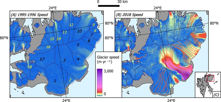
1432                                                 W. Zheng: How marine-terminating glaciers respond to lubricated beds

dynamics over multiple years. For example, the recent ex-           2.1    Perturbation due to a permanent change of basal
tensive formation of supraglacial lakes in the GrIS can open               conditions
new moulins that last for years and contribute to long-lived
speedups (e.g., Hoffman et al., 2018). During several glacier       We set up a glacier with the following initial values along
surge events in Svalbard and the Russian Arctic, initial flow       its 1D flowline profile: speed (U0 ), thickness (H0 ), flux (q0 ),
speedups have also created highly crevassed glacier surface         surface slope (α0 ), and bed friction term (K0 ). These values
and led to further speedups by additional meltwater rout-           vary along the flowline distance x (positive towards down-
ing (e.g., Dunse et al., 2015; Strozzi et al., 2017a; Zheng         stream) and do not vary with time (i.e., steady state). We as-
et al., 2019; Sánchez-Gámez et al., 2019). These events po-         sume that the ice is purely sliding on the bed and does not
tentially alter the basal conditions by allowing meltwater to       have any internal deformation, that is,
reach the bed in all seasons, but their interannual impact is
still less constrained (Kehrl et al., 2017). In addition, glacier   q 0 = U 0 H0 .                                                (1)
geometry plays a vital role in how a glacier responds to an
                                                                    The glacier speed can be further represented using the hard-
external perturbation (Carr et al., 2017; Kehrl et al., 2017),
                                                                    bed sliding law (Weertman, 1957):
but only terminus disruption has been physically well docu-
mented and explained (McFadden et al., 2011; Felikson et al.,       U0 = K0 H0m α0m ,                                             (2)
2017, 2021). Whether some glaciers are more sensitive to
basal lubrication than others owing to their geometry is not        where m is the flow-law constant and is set to 3 in this study.
well known.                                                            At t = 0, the bed condition changes and the friction term
   To better understand how much and how fast a glacier             becomes K0 + K1 . The second term K1 denotes the amount
responds to basal lubrication and its relationship to glacier       of change and is positive for a lubrication scenario. There is
geometry, this paper presents a physical model with a               no initial elevation change associated with this event. We also
1D framework along flowlines formulating the subsequent             assume that this is a one-time change and is uniform over the
change (in terms of both glacier speed and surface elevation)       glacier, so K1 is a constant. The subsequent change of speed,
after the glacier bed is suddenly lubricated. We use an ex-         elevation, flux, and slope are represented as U1 , H1 , q1 , and
isting glacier perturbation model (Zheng et al., 2019) and          α1 respectively. Unlike K1 , these quantities vary along the
replace the initial thinning condition with a step reduction        glacier channel and over time. Assuming zero local surface
of basal friction along the glacier channel. This new model         mass balance and zero local stress imbalance (e.g., Felikson
identifies key parameters that dominate elevation change rate       et al., 2017; Zheng et al., 2019), the conservation of mass can
and ice flow acceleration. Then, using data from the GrIS           be expressed as
and Austfonna ice cap, Svalbard, we derive these parameters
for each glacier basin and compare them with glacier speed          ∂H1    ∂q1
                                                                        =−     .                                                  (3)
change over 20 years. The entire processing workflows, in-           ∂t    ∂x
cluding data fetching, all calculations, and figure scripts, are    Taking the total derivative of q1 with respect to t yields
available on Github (https://github.com/whyjz/pejzero, Zen-
odo DOI: https://doi.org/10.5281/zenodo.5641953) and are                   ∂q0      ∂q0      ∂q0
compiled as a Jupyter Book ready to be cloud executed using         q1 =       K1 +     H1 +     α1 .                             (4)
                                                                           ∂K       ∂H       ∂α
the MyBinder service for full reproducibility (Project Jupyter
et al., 2018; Executable Books Community, 2020).                    If we assume a much more gentle slope of the bedrock than
                                                                    that of the ice surface (Felikson et al., 2017; Zheng et al.,
                                                                    2019), the surface slope can also be expressed as the first
2   Model development                                               derivative of ice thickness:

We build the model on the perturbation theory developed by                   ∂H1
                                                                    α1 = −       .                                                (5)
Nye (1963), Bindschadler (1997), Felikson et al. (2017), and                  ∂x
Zheng et al. (2019). Our goal in this section is to formulate       Plugging Eqs. (1), (2), (4), and (5) into Eq. (3) yields
the change rate of ice elevation ( dH  1                  dU1
                                     dt ) and ice speed ( dt )
after a glacier bed is lubricated permanently. In this new          ∂H1     K1   ∂H0      ∂α0      ∂C0
                                                                        = − (C0      + D0     )−       H1
model, basal lubrication is considered as a sudden perturba-         ∂t     K0    ∂x      ∂x        ∂x
tion without initial elevation change. The variables defined in
                                                                                              ∂ 2 H1

                                                                               ∂D0 ∂H1
the model are listed in Table 1.                                        − C0 −          + D0         ,                            (6)
                                                                                ∂x   ∂x        ∂x 2
                                                                    where
                                                                            ∂q0
                                                                    C0 =                                                          (7)
                                                                            ∂H

The Cryosphere, 16, 1431–1445, 2022                                                     https://doi.org/10.5194/tc-16-1431-2022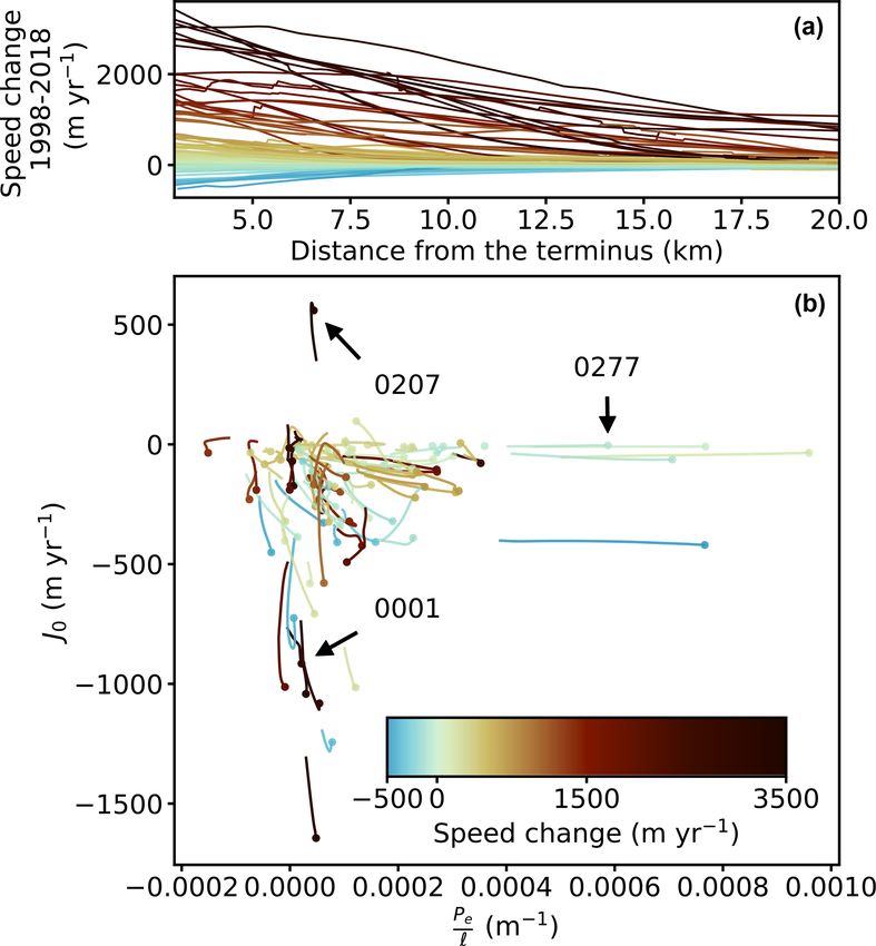
W. Zheng: How marine-terminating glaciers respond to lubricated beds                                                              1433

Table 1. Variables used in the perturbation model defined in this study. In the dimension column, L is length and T is time. The prime
notation used in the text denotes the partial derivative of a variable with respect to x; for example, H10 ≡ ∂H 1
                                                                                                              ∂x .

                         Variable    Definition                                                       Dimension
                         x           Distance along a 1D glacier flowline towards terminus            L
                         t           Time after perturbation                                          T
                         m           Flow law constant                                                None
                         U0 (x)      Glacier speed before perturbation                                LT −1
                         U1 (x, t)   Change of glacier speed after perturbation                       LT −1
                         K0 (x)      Basal friction term before perturbation                          Lm−1 T −1
                         K1          Change of basal friction after perturbation (assumed constant)   Lm−1 T −1
                         H0 (x)      Glacier thickness before perturbation                            L
                         H1 (x, t)   Change of glacier thickness after perturbation                   L
                         α0 (x)      Glacier slope before perturbation                                None
                         α1 (x, t)   Change of glacier slope after perturbation                       None
                         q0 (x)      Flux before perturbation                                         L2 T −1
                         q1 (x, t)   Change of flux after perturbation                                L2 T −1
                         C0 (x)      ≡ ∂q0 /∂H                                                        LT −1
                         D0 (x)      ≡ ∂q0 /∂α                                                        L2 T −1
                         J0 (x)      ≡ C0 H00 + D0 α00                                                LT −1
                         Pe(x)       Péclet number, see Eq. (14)                                      None
                         `           Characteristic length (length of perturbation)                   L

and                                                                     At t = 0,
        ∂q0                                                             ∂U1            K1 C0
D0 =        .                                                  (8)          |t=0 = −J0       .                                     (13)
        ∂α                                                               ∂t            K0 H0
Since H1 (t = 0, x) = 0,                                                Similar to the elevation change, J0 is inversely proportional
                                                                        to the initial glacier acceleration. If two glacier beds are lu-
∂H1         K1
    |t=0 = − J0 ,                                              (9)      bricated with the same amount of K1 /K0 , the glacier with a
 ∂t         K0                                                          higher absolute value of J0 (i.e., |J0 |) will be more unstable
where                                                                   as the initial speed and elevation change rates are higher.
                                                                           Also, from Eq. (9) we can predict a subsequent eleva-
                         ∂q0 ∂H0 ∂q0 ∂α0
J0 = C0 H00 + D0 α00 =          +        .                   (10)       tion change after t = 0. At this point, the last three terms in
                         ∂H ∂x    ∂α ∂x                                 Eq. (6) begin to take part in the elevation change rate. The
2.2    J0 and Péclet number (Pe)                                        second term of Eq. (6) represents an exponential decay of
                                                                        the change rate, and the third and the fourth terms indicate
Equation (9) indicates that the ratio of K1 to K0 and the value         advective and diffusive migration of elevation perturbation,
of J0 both determine the initial elevation change rate. In a            respectively. The coefficients of the latter two terms deter-
lubricating scenario, both K1 and K0 are positive, and the              mine the relative strength between advection and diffusion,
initial response of dH  1
                      dt is inversely proportional to J0 .
                                                                        with the ratio defined as the Péclet number, Pe:
   To relate J0 to the glacier speed change, we start from the
                                                                               C0 − D00
change of flux and assume U1 >>H1 . This can be justified by            Pe =            `,                                         (14)
many observations of glacier destabilization as the amount                       D0
of speed change is usually one to two orders of magnitude               where ` is the length of a perturbation. If Pe is much higher
higher than the amount of elevation change (e.g., McMillan              than 0, forward advection will dominate, and any perturba-
et al., 2014; Willis et al., 2018). Therefore,                          tion of ice thickness will only propagate downstream. This
                                                                        prohibits destabilization in the upper stream if thinning or
q1 = U1 H0 + U0 H1 ≈ U1 H0 .                                 (11)       glacier retreat initiates near the terminus. On the other hand,
As K1 is a constant, we can derive the glacier speed change             if Pe ∼ 0 or is negative, either diffusion or backward advec-
using Eqs. (4), (5), (7), (8), and (11):                                tion takes place, and a thickness perturbation at the terminus
                                                                        can propagate upstream, changing the dynamics of the en-

∂U1     1 ∂q1         1        ∂H1        ∂ ∂H1                         tire glacier. Hence, we consider a glacier with a low Pe more
     =           =         C0       − D0          .     (12)            vulnerable than one with a high Pe.
 ∂t    H0 ∂t         H0         ∂t       ∂x ∂t

https://doi.org/10.5194/tc-16-1431-2022                                                        The Cryosphere, 16, 1431–1445, 2022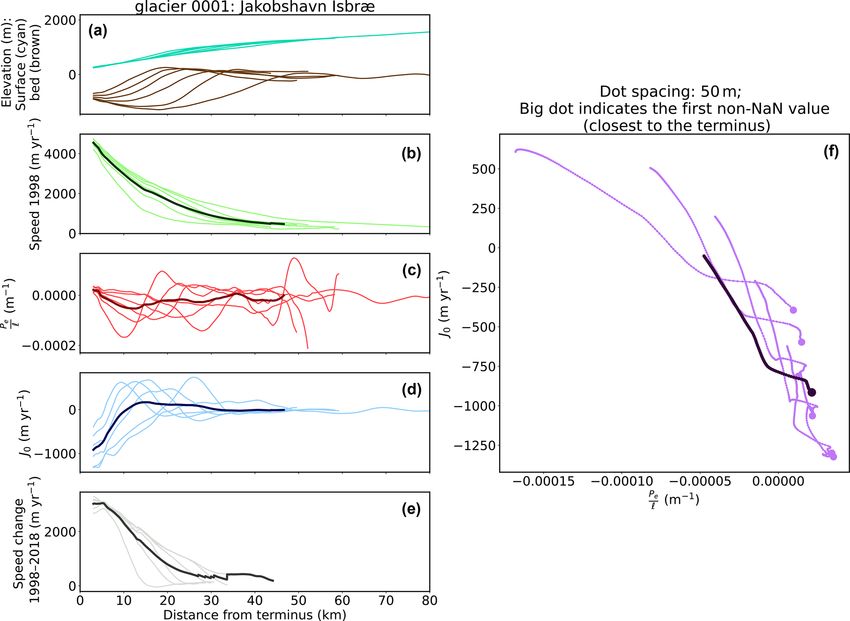
1434                                                 W. Zheng: How marine-terminating glaciers respond to lubricated beds

   Combining Eqs. (1), (2), (7), and (8) with Eq. (14), we          3     Data and methods for validating the model
can express Pe in terms of ice speed, elevation, and surface
slope (see Sect. S4 of Zheng et al., 2019, Eqs. 11 to 16 for        To test if the model is suitable for evaluating marine-
derivation details):                                                terminating glaciers, we derive observed Pe/` and J0 for
                                                                    outlet glaciers in the GrIS and Austfonna ice cap, Svalbard.
       h (m + 1)α
                    0       U00 H00 α00 i                           These two regions are selected primarily because surface el-
Pe =                    −      −   +      `.                (15)
          mH0               U 0 H0 α 0                              evation, bed elevation, and glacier speed data necessary for
                                                                    our calculation are publicly available. We compare the re-
The final assumption we adopt in the model is α00 = ∂α     0
                                                         ∂x ≈ 0
                                                                    sults with the NASA MEaSUREs ITS_LIVE glacier veloc-
as the estimated value from the data we use in this paper           ity (Gardner et al., 2018, 2019) and frontal retreat records
is essentially small. For example, α00 of the glacier profile       (Wood et al., 2021) spanning over 20 years and determine if
shown in Fig. 3 is only around 10−6 –10−7 m−1 for the first         both Pe/` and J0 are indicative of the vulnerability to basal
100 km, and the last term in Eq. (15) is roughly an order           lubrication.
less than the sum of the first three terms. In practice, this as-
sumption might be necessary because α00 is highly sensitive         3.1    Greenland ice sheet
to local slope change and may not reflect the glacier’s overall
mechanism to dissipate the perturbation. With this assump-          We use the data set published with Felikson et al. (2021),
tion, Eq. (15) can be reduced to:                                   which provides well-constrained flowline data for Green-
                                                                    land’s 141 marine-terminating glaciers and their branches
Pe

       (m + 1)α0 U00 H00
                                                                   (187 basins in total, Fig. 1). These glaciers scatter around
   ≈            −   −      .                                (16)    the ice sheet and provide a diverse sampling over various
`        mH0      U0 H0
                                                                    climate and oceanic factors. The data set contains six pri-
Note we now express the Péclet number as the form of Pe             mary flowline shapes for each glacier basin, with vertices
                                                        ` as
we do not focus on a particular perturbation length and in-         sampled every 50 m along the flowlines. We use surface ele-
stead plan to evaluate the general tendency for the ice flow        vations at each vertex, sampled from the Greenland Ice Map-
to dissipate any length of perturbations. Compared with the         ping Project (GIMP, Howat et al., 2014). The GIMP surface
past models, the expression of Pe in this model has an addi-        elevations come from multiple remote sensing sources and
             U0                                                     are coregistered with elevations acquired by the Ice, Cloud,
tional term U00 , implying its relationship to spatially chang-     and land Elevation Satellite (ICESat), thus best representing
ing basal conditions. This extra dependency on glacier speed        the ice sheet elevations during 2003–2009. The flowline ver-
also suggests that Pe is a changing variable and needs to be        tices also contain the glacier bed elevations, sampled from
re-calculated if ice flow speeds up or slows down (see Dis-         the BedMachine v3 subglacial topography (Morlighem et al.,
cussion for more details).                                          2017). Although BedMachine v3 uses the source data col-
   With the same assumption about α00 , the expression of J0        lected from 1993 to 2016, we assume that the bed elevations
(Eq. 10) can be also reduced to:                                    are stable over time and can represent any year in that period.
                                                                    To acquire U0 and glacier speed change at each flowline ver-
J0 ≈ C0 H00 = (m + 1)U0 H00 ,                               (17)
                                                                    tex, we manually sample the annually mosaicked ITS_LIVE
                                                                    glacier speed data from 1998 and 2018, respectively. The
which is proportional to the product of ice speed and the gra-
                                                                    ITS_LIVE data are derived from Landsat 4, 5, 7, and 8 im-
dient of ice thickness along the flowline. A typical glacier
                                                                    ages using the autoRIFT feature tracking software (Gardner
thins toward the terminus, corresponding to a negative H00
                                                                    et al., 2018; Lei et al., 2021). Finally, each vertex of a flow-
and J0 . According to Eq. (13), a negative J0 suggests that
                                                                    line has the following key parameters: surface elevation, bed
when a lubricating scenario takes place, the glacier might
                                                                    elevation, glacier speed in 1998, and speed difference be-
speed up to accommodate the change. From Eq. (9) we can
                                                                    tween 1998 and 2018.
see that the glacier will also get thickened (except at the di-
                                                                       We prepare and process the input data for each flowline
vide) as thicker ice is sliding and replaces thinner ice down-
                                                                    using the following steps:
stream.
   To summarize, two parameters Pe and J0 are derived from              1. As the 1998 speed data do not cover the entire ice sheet,
the 1D basal lubrication model. J0 represents the strength                 we remove flowlines with only 20 speed readings or less
of initial response to basal lubrication, and Pe gives insights            from the input list.
into the mode of mass transport after elevation change oc-
curs. Glaciers with a high |J0 | and a low Pe (∼ 0 or negative)         2. Locate vertices with NoData speed values along the
are more vulnerable to basal lubrication as reduced friction               flowlines and perform a linear interpolation to fill the
can lead to a high initial acceleration and elevation change               missing values. We do not extrapolate the glacier speed;
rate, which will then propagate to the entire glacier via diffu-           therefore, the NoData vertices at both ends of the flow-
sion or negative advection.                                                line are still preserved after this step.

The Cryosphere, 16, 1431–1445, 2022                                                      https://doi.org/10.5194/tc-16-1431-2022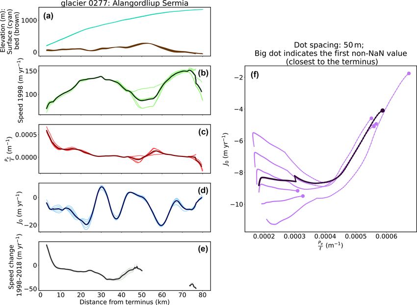
W. Zheng: How marine-terminating glaciers respond to lubricated beds                                                         1435

 3. Remove flowlines with only 280 valid vertices or less          Cryospheric Sciences (IACS). We use the Austfonna DEM
    from the input list. A valid vertex should contain all key     from 1996 (Moholdt and Kääb, 2012), velocity from 1995–
    parameters and no NoData Values.                               1996 (Dowdeswell et al., 2008), and ice thickness from 1996
                                                                   (Dowdeswell et al., 1986; Farinotti et al., 2017), all included
 4. To avoid the effect of small sloping change, we smooth         in the ITMIX data set. Eight out of 11 marine-terminated
    the surface elevation, bed elevation, glacier speed data,      glaciers (basin-1, -3, -4, -5, -6, -7, -10, and -17; Fig. 2) are
    and their derivatives using the Savitzky–Golay filter          selected for the analysis; the exceptions are basin-2, -8, and
    with a window size of 251 vertices (12.5 km) (Savitzky         -9 owing to their small length roughly equal to the smoothing
    and Golay, 1964; Felikson et al., 2021). We do not apply       window. We construct six glacier flowlines based on the 2018
    the smoothing filter to data 0–3 km from the terminus          glacier velocity from the ITS_LIVE annual velocity mosaics
    owing to insufficient sampling points within the win-          (Fig. 2b) and sample ITMIX glacier elevation, ice thickness,
    dow size. These unfiltered data will not be used for the       and glacier speed data every 50 m along each flowline. Then
    next step.                                                     we follow the same workflow for the outlet glaciers in GrIS
 5. Derive Pe/` and J0 along each flowline using Eqs. (17),        (see the previous section) and finally compare Pe/` and J0
    (16), and parameters representative of the glacier geom-       with the ITS_LIVE 2018 glacier speeds.
    etry/speed from 1998. As we empirically derive Pe/`
    and J0 for each basin and compare them on the same             4     Results
    plot, the results will be insensitive to the selected value
    of m and the sliding law (Felikson et al., 2021).              4.1    Variation within a single basin
 6. We also need to include glacier retreat in our analy-          Figures 3 and 4 provide example results within a single
    sis to better distinguish the relationship between basal       basin, showing both input data and the values of Pe/` and
    lubrication and speedups. Thus, we use the Greenland           J0 along six major flowlines. The average frontal speed at
    Marine-Terminating Glacier Retreat Data (Wood et al.,          Glacier 0001 (Jakobshavn Isbræ; 69.18◦ N, 49.76◦ W, Figs. 1
    2021), which contain temporal evolution of terminus            and 3) has changed from ∼ 4000 to ∼ 7000 m yr−1 dur-
    positions derived from Landsat 5, 7, and 8 images for          ing the studied period, suggesting a destabilized status. The
    226 glaciers. We use QGIS to manually measure the ter-         value of Pe/` of individual flowlines ranges within ±2 ×
    minus retreat between 1988 and 2018 for each glacier at        10−4 m−1 for the first 20 km from the terminus, but the av-
    its center flowline.                                           erage value is more constrained roughly between −5 × 10⁻⁵
 7. Compare Pe/` and J0 with the frontal retreat and the           and 2×10⁻⁵ m−1 for the first 10 km. Compared with Pe/`, J0
    speed change between 1998 and 2018.                            changes more quickly throughout the first 20 km, from about
                                                                   −1000 to 170 m yr−1 . If we plot J0 versus Pe/` (Fig. 3f)
                                                                   along the first 10 km from the terminus, the average values
3.2   Austfonna ice cap, Svalbard                                  will roughly form a line going from lower right to upper left
                                                                   in the figure.
We perform the same analysis for the marine-terminating               On the other hand, glacier 0277 (Alangordliup Sermia,
glaciers of Austfonna, a polythermal ice cap located in NE         68.95◦ N, 50.22◦ W, ∼ 30 km south of Jakobshavn Isbræ;
Svalbard. Austfonna is only about 100 km wide and is con-          Figs. 1 and 4) is more stable than glacier 0001 as the amount
sidered to have a more uniform climate and oceanic factors         of the speed change in the past two decades is only 0–
than the GrIS, but its marine outlet glaciers have exhibited       40 m yr−1 and is constrained at the first 6 km from the termi-
diverse speed histories in the past 20 years (Fig. 2). For         nus. Pe/` ranges from 2 × 10⁻⁴ to 6 × 10⁻⁴ m−1 within the
instance, the glacier speed of basin-3 (Storisstraumen) in-        first 10 km, which is roughly 10 times the values from Jakob-
creased 45-fold during the past two decades, likely triggered      shavn Isbræ. Also, the slow glacier speed in 1998 directly re-
by feedback between summer melt, crevasse formation, and           sults in low |J0 | (only ∼ −10 m yr−1 ) compared with Jakob-
basal lubrication (McMillan et al., 2014; Dunse et al., 2015;      shavn Isbræ. These results are supportive for glacier 0277
Gong et al., 2018). The other surge-type glaciers include          having a stable condition during the study period. Interest-
basin-1 (Bråsvellbreen) and basin-17 (Etonbreen), and the          ingly, the speed change pattern resembles Pe/` at the first
last surge periods of both glaciers are around 1938 (Schytt,       10 km. The glacier might have dealt with frontal or basal per-
1969; Hagen et al., 1993; Dowdeswell et al., 2008). The other      turbation through advection, as indicated by a large Pe.
glaciers of Austfonna do not have a surge history, but many           The results of the other GrIS and Aust-
of them (e.g., basin-2, -5, -7, and -10) have also significantly   fonna glaciers are available in Github-Zenodo
increased the flow speed since 1996, as seen from Fig. 2.          (https://doi.org/10.5281/zenodo.5641953).
   To calculate Pe/` and J0 , we use the Ice Thickness Mod-
els Intercomparison eXperiment (ITMIX) data set (Farinotti
et al., 2017), hosted by the International Association of

https://doi.org/10.5194/tc-16-1431-2022                                                 The Cryosphere, 16, 1431–1445, 2022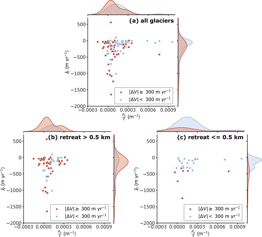
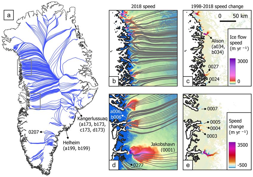
1436                                                   W. Zheng: How marine-terminating glaciers respond to lubricated beds

Figure 1. Greenland glacier flowlines used in this study. (a) Location of all selected flowlines from 104 outlet glaciers or glacier branches.
Gray boxes indicate map locations for panels (b)–(e). (b, c) The closer view of the flowline distribution, speed from 2018, and speed change
during 1998 and 2018 at NW Greenland, a place with the most flowlines across the ice sheet. (d, e) Same panels as (b) and (c) but for W
Greenland where Jakobshavn Isbræ is located in the bottom. The glacier speeds from 1998 and 2018 are both sampled from the ITS_LIVE
data set. Major glaciers and most glaciers in the zoom-in panels are labeled with names and IDs used in the source data set. Panels (b)–
(e) share the scale bar illustrated in panel (c).

Figure 2. Austfonna ice cap, Svalbard, and glacier flowlines. (a) ITMIX glacier speed in 1995–1996. Each glacier basin is labeled with a
number as per Dowdeswell et al. (2008), and glaciers with black numbers are analyzed in this study. (b) ITS_LIVE mosaicked glacier speed
in 2018. For each selected basin, we generate six flowlines and plot them on the map as red lines. Glacier outlines are from the Randolph
Glacier Inventory (RGI) version 6.0 (RGI Consortium, 2017). (c) Map of Svalbard, Norway; the red box highlights the location of the
Austfonna ice cap. Panels (a) and (b) share the scale bar at the top of the figure.

The Cryosphere, 16, 1431–1445, 2022                                                            https://doi.org/10.5194/tc-16-1431-2022
W. Zheng: How marine-terminating glaciers respond to lubricated beds 1437
Figure 3. Example results from glacier 0001 (Jakobshavn Isbræ, 69.18◦ N, 49.76◦ W). (a) Surface elevation (cyan) and bed elevation (brown).
(b) Surface speed in 1998. (c) Pe/`. (d) J0 . (e) Speed change between 1998 and 2018. These plots show all six flowline profiles from a single
basin in respect of the distance from the glacier terminus. The thick lines represent the average of these flowlines. (f) J0 versus Pe/` along
the first 10 km from the terminus. The big dots represent values at 3 km or the valid values closest to the terminus, and the small dots are
plotted every 50 m along the flowline.
4.2 Pe & J0 versus glacier speed change on the speed change at 3 km as well (Fig. 5b). Glaciers with
low speed change (pale color curves) tend to cluster around
This study focuses on the parameter variations close to the the area where J0 ≈ 0 m yr−1 and Pe/` > 0.0001 m−1 . Most
glacier terminus for two reasons. First, crevasses and moulins of these curves are near horizontal on the plot, indicating
are more likely to form at the terminus region via hydrofrac- a small change of J0 and a large change of Pe/` at the
ture than at higher elevations (Poinar et al., 2015). Therefore, glacier front. On the other hand, glaciers with high speed
additional meltwater routing can alter the basal conditions change (warm- or cold-color curves, including accelerated
over multiple years. In addition, the J0 tends to be small for and decelerated glaciers) seem to cluster together in a differ-
the upper regions of all glaciers where the ice flow is slow, ent area where J0 is much more negative and Pe/` ≈ 0 m−1 .
making this metric less distinctive from one basin to another. These curves generally show a vertical orientation indicating
Considering the limit of spatial smoothing in the processing changing J0 and constant low Pe/` along the glacier flowline.
workflow (see Sect. 3.1, step 4), we select the data at 3 km To further illustrate the clustering trend, we arbitrarily se-
from the terminus for the following intercomparison. Owing lect a speed change threshold of ±300 m yr−1 and classify
to the incomplete spatial coverage of ITS_LIVE data from the glaciers based on their speed change at 3 km. The thresh-
1998, only 104 out of 187 GrIS glacier basins have valid val- old value is determined in order to give each classification
ues of Pe/` and J0 at this terminus distance (Fig. 1). roughly the same number of samples. Note that glaciers with
Although most of these glaciers have sped up during the significant slowdown or speedup are classified into the same
20 years, 26 glaciers slowed down by up to −522 m yr−1 group because a glacier vulnerable to basal lubrication would
(Fig. 5a). To illustrate Pe/` and J0 at the glacier front and also be sensitive to recovering basal conditions from a lu-
their varying direction along the flowline, we plot J0 versus brication event. Fifty-four glaciers have an absolute value
Pe/` using ball-head-pin-like curves. Each curve represents of speed change ≥ 300 m yr−1 , and the other 50 glaciers
the average J0 and Pe/` values of one glacier basin at 3– are considered more stable with an absolute value of speed
5 km with the head mark located at 3 km, color-coded based change < 300 m yr−1 . We plot J0 against Pe/` using the val-
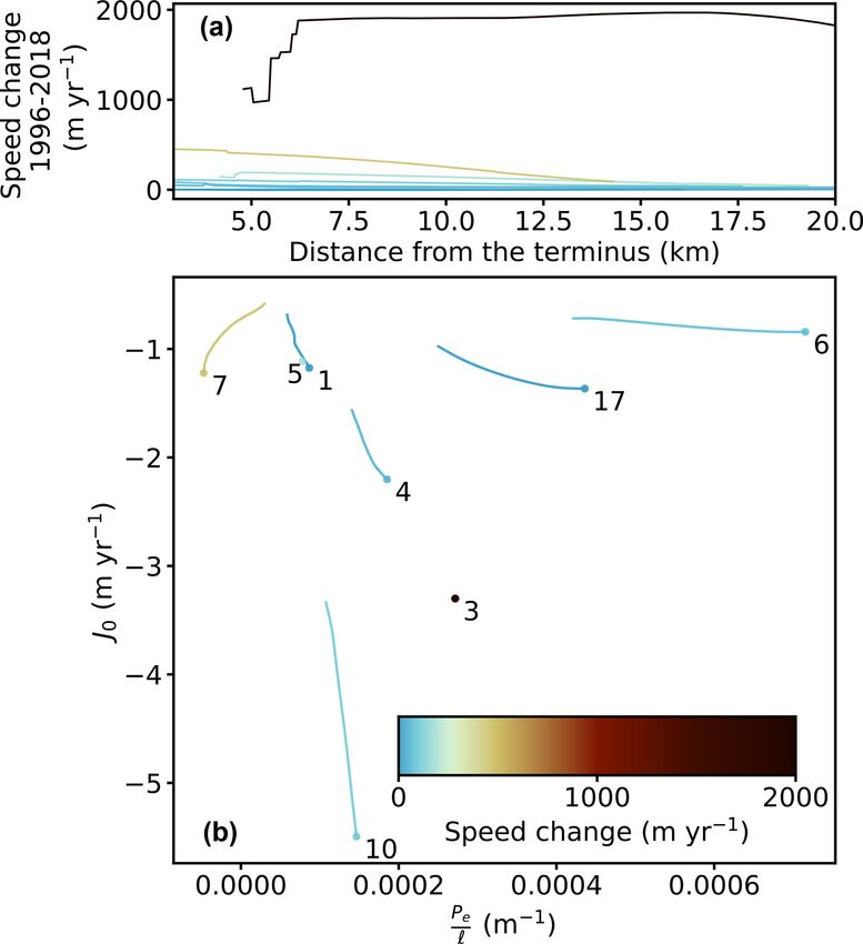
https://doi.org/10.5194/tc-16-1431-2022 The Cryosphere, 16, 1431–1445, 20221438 W. Zheng: How marine-terminating glaciers respond to lubricated beds Figure 4. Example results from glacier 0277 (Alangordliup Sermia, 68.95◦ N, 50.22◦ W). See Fig. 1 for geographical location and Fig. 3 for a detailed description of each panel. ues from 3 km as well as the Gaussian kernel density esti- Among all the glacier outlets, glacier 0207 (65.17◦ N, mates of each classification for both J0 and Pe/`. The re- 41.16◦ W; Fig. 1a) seems to be unusual as it is the only one sults using all glaciers (Fig. 6a) indicate that two classifica- with J0 over 100 m yr−1 (Fig. 5b). A positive J0 requires a tions have a slightly different distribution for J0 and Pe/`. decreasing ice thickness from terminus to upstream (Eq. 17), The unstable glaciers (red group) have J0 and Pe/` distribu- which seems to indicate a steeper bed than the glacier sur- tions peaked at ∼ −200 m yr−1 and ∼ 0.00003 m−1 respec- face. In our analysis, glacier 0207 is considered an example tively, whereas the peaks of stable glaciers (blue group) shift with large |J0 |, despite having a different sign than the other to higher values to ∼ −50 m yr−1 for J0 and ∼ 0.00013 m−1 glaciers. However, additional data from more glaciers would for Pe/`. Despite the peak shift being small compared with be required to fully characterize the glaciers with positive J0 the distributions themselves, the difference is statistically sig- and their sensitivity to basal lubrication. nificant found by the Kolmogorov–Smirnov statistic (p = We adopt the same method from Fig. 5 to plot the results 0.003 and 0.006 for J0 and Pe/`, respectively; see the Fig. 6 from eight marine-terminating glaciers in Austfonna (Fig. 7). Jupyter Book page for details). As the major cause of glacier As all glaciers have accelerated at the terminus for the past speedups has been attributed to terminus retreat (King et al., two decades, we adjust the color code so that blue repre- 2020), we further group the glaciers by the distance of ter- sents low change and other colors represent high change. minus retreat. Figure 6b plots only the glaciers with a retreat For basin-3 and -5, there are no valid measurements at 3 km, larger than 0.5 km, and the separation between two glacier and we only mark the first valid measurements from 7.3 and groups in terms of J0 and Pe/` becomes much less signifi- 6.7 km, respectively, as single points on the plot. Similar to cant (p = 0.366 and 0.050 respectively). On the other hand, the GrIS, glaciers with higher speed change (basin-3, -5, -7, Fig. 6c shows the J0 and Pe/` distributions for glaciers with and -10) roughly occupy the lower left side of the panel a retreat ≤ 0.5 km. Only seven glaciers with little or no re- where Pe/` and J0 are small or more negative, and glaciers treat have accelerated over 300 m yr−1 , which might not be with lower speed change (basin-1, -4, -6, and -17) fall on a enough to determine the significance of separation for Pe/` different corner, where Pe/` and J0 are larger. However, |J0 | (p = 0.255). However, it is clear to see two groups divided of all eight glaciers have values between 0 and 10 m yr−1 , by the value of J0 in the plot (p = 2 × 10⁻⁵ ). much lower than those from the GrIS (see Fig. 5, where The Cryosphere, 16, 1431–1445, 2022 https://doi.org/10.5194/tc-16-1431-2022
W. Zheng: How marine-terminating glaciers respond to lubricated beds                                                              1439

                                                                         these glaciers. Nevertheless, the separation of peaks at dif-
                                                                         ferent Pe/` values suggests that the diffusive strength of ice
                                                                         flow might still play a major role in the decades-long speed
                                                                         changes. For glaciers with a more stable terminus position,
                                                                         the clear separation of J0 (Fig. 6c) supports basal lubrication
                                                                         as a primary cause of glacier speedups and likely highlights
                                                                         the importance of the initial response to changing basal con-
                                                                         ditions. Even if a glacier has a low P0 and allows diffusion-
                                                                         dominating dynamics, a small |J0 | prohibits much elevation
                                                                         and speed change under a lubrication scenario (Eq. 9).
                                                                            The other factor that might affect the tendency of Pe/`
                                                                         and |J0 | we see in Fig. 6 is whether the basal lubrication
                                                                         takes place within the study period. Although melt-induced
                                                                         speedups are common for GrIS glaciers (e.g., van de Wal
                                                                         et al., 2008; Bartholomew et al., 2010; Kehrl et al., 2017;
                                                                         Rathmann et al., 2017; Seddik et al., 2019), not all 104
                                                                         glacier basins analyzed here have been studied well enough
                                                                         to identify when and where a glacier responds to changing
                                                                         basal conditions. A glacier with low Pe/` and high |J0 | can
                                                                         remain stable if no basal lubrication has taken place in the
                                                                         past decades, mixing up the distributions in Fig. 6. Also, the
                                                                         Pe/` and |J0 | patterns at the glacier front may not represent
Figure 5. (a) Speed change along Greenland glacier flowlines             the entire glacier length. If moulins can form at a higher ele-
within the first 20 km from the terminus. Each line represents the       vation than previously thought owing to the warming climate
average value of a single glacier basin and is color coded based on      and widespread supraglacial lakes (Hoffman et al., 2018),
the speed change value at 3 km (the first valid data point after the     it might be necessary to reassess the Pe/` and |J0 | patterns
Savitzky–Golay filter is applied). (b) The average J0 versus Pe/` at     within a wider range of flowline distance.
3–5 km from the terminus. The value at 3 km is marked with a big            The three surge-type glaciers of Austfonna (basin-1, -3,
dot. Each line uses the same color code from (a). The glacier basins     and -17) do not cluster in Fig. 7. Compared with the other
presented in Figs. 3 (0001) and 4 (0277), as well as one extra glacier   two glaciers, basin-3 has a higher flow speed in 1995–1996,
basin (0207) are annotated.
                                                                         resulting in a slightly more negative J0 . It has had an un-
                                                                         usually long surge evolution over two decades as well: the
                                                                         ice flow speed has gradually increased since the mid-1990s
|J0 | ranges from 0 to over 1500 m yr−1 ). This is because all
                                                                         (Dowdeswell et al., 2008; McMillan et al., 2014) and reached
eight glaciers are slowly moving in 1996, resulting in a low
                                                                         a peak velocity of ∼ 6500 m yr−1 in 2013 (Dunse et al.,
|J0 | according to Eq. (17). It is also interesting that basin-1
                                                                         2015). The sustaining high flow speed has been attributed
(Bråsvellbreen) and basin-5 have similar J0 versus Pe/`, but
                                                                         to meltwater routing through crevasses formed during the
basin-5 has a speed change roughly ten times greater than
                                                                         speedup (Dunse et al., 2015; Gong et al., 2018). As the ad-
basin-1. Since basin-1 had a surge record back in 1936–1938
                                                                         ditional supply of surface melt can alter the behavior of a
(Schytt, 1969) and is currently in the quiescent stage, its low
                                                                         surge-type glacier by reaching a steady state balancing mass
J0 and Pe/` values might indicate a future instability when a
                                                                         and enthalpy conservation through thinner and faster-moving
surge is triggered internally or externally.
                                                                         ice (Benn et al., 2019), basin-3 may have entered an ice
                                                                         stream-like regime with higher sensitivity to changing basal
5     Discussion                                                         conditions. This might explain why basin-3 is away from
                                                                         the other two surge-type but currently quiescent glaciers on
5.1    Separation of glacier groups on the J0 versus Pe/`                Fig. 7. Nevertheless, additional analysis and tests will be re-
       plot                                                              quired before inferring a general vulnerability for surge-type
                                                                         glaciers to basal lubrication.
For the GrIS, the J0 versus Pe/` plots (Figs. 5–6) seem to
capture the characteristics of glaciers vulnerable to basal lu-          5.2   Characteristics of glaciers vulnerable to basal
brication. GrIS glaciers with more negative J0 and Pe/` in                     lubrication
1996–1998 are more likely to speed up in the next 20 years.
This tendency is not obvious for glaciers with a significant             Both Pe and J0 depend on the ice thickness and flow speed
retreat (Fig. 6b), possibly because instead of changing basal            (Eqs. 16 and 17), but with a different relationship. Assuming
conditions, it is the retreat dominating the flow dynamics of            a monotonous decrease in glacier thickness toward the ter-

https://doi.org/10.5194/tc-16-1431-2022                                                       The Cryosphere, 16, 1431–1445, 2022
1440 W. Zheng: How marine-terminating glaciers respond to lubricated beds Figure 6. Distribution of J0 and Pe/` for (a) The Greenland ice sheet’s 104 glacier basins analyzed in this study; (b) a subset of panel (a) in- cluding only basins with a frontal retreat > 0.5 km during 1998–2018; (c) a subset of panel (a) including only basins with a frontal retreat ≤ 0.5 km during 1998–2018. These plots are similar to Fig. 5b but only show the values at 3 km from the terminus. Each mark is classified based on the 300 m yr−1 threshold of speed change. The joint plots show the Gaussian kernel density estimate along both axes for each class. minus (i.e., no overdeepening area), glaciers with thicker ice minus perturbation to propagate to a certain inland distance and a faster flow yield lower Pe and higher |J0 | and thus are where Pe becomes larger (Felikson et al., 2017, 2021). For more susceptible to basal lubrication. However, the thickness an outlet glacier in the GrIS, it is probably common to have change along the flowline (H 0 ) has a competing contribution terminal perturbation and changing basal conditions in ef- to Pe and J0 : a greater change (i.e., a more negative H 0 ) in- fect at the same time (as indicated by Jakobshavn Isbræ for creases both Pe and |J0 |. Glaciers with a very negative H 0 example; Joughin et al., 2008; Khazendar et al., 2019; Riel may not likely be activated through intense diffusion (which et al., 2021). In this case, Pe reflects a general vulnerabil- is also suggested to be true for a terminus perturbation sce- ity to elevation perturbations and is indistinguishable from nario in Felikson et al., 2021), but a collapse-like destabi- the source forcing. On the other hand, J0 as a new term lization is still possible at the terminus or a localized region in the lubrication-induced perturbation model seems to be along the glacier owing to its high |J0 |. For a glacier with an exclusively related to the basal sensitivity as indicated by overdeepening zone, increased ice thickness again lowers Pe Fig. 6b and c. Nevertheless, J0 might still be a key factor for and raises |J0 |, making the glacier more vulnerable to basal a glacier only subject to the ocean–ice interaction. As warm lubrication at the overdeepened area. subsurface water-induced thinning debuttresses the glacier Despite having an additional associating factor J0 in the front and increases the longitudinal stretching and glacier model, inferences made to the Péclet number in this study speed (Holland et al., 2008), new crevasses can provide ad- is similar to the previous models based on the perturbation ditional routes for surface melt accessing and lubricating the theory. A low or negative Pe allows an ocean-induced ter- bed (Gagliardini and Werder, 2018; Gong et al., 2018). The The Cryosphere, 16, 1431–1445, 2022 https://doi.org/10.5194/tc-16-1431-2022
W. Zheng: How marine-terminating glaciers respond to lubricated beds                                                                1441

                                                                          the glacier more sensitive to any following change in basal
                                                                          conditions. A potential example to illustrate this feedback is
                                                                          the Vavilov ice cap, Severnaya Zemlya, Russia. The west-
                                                                          ern marine outlet of this ice cap was moving at less than
                                                                          1 km yr−1 with no apparent summer speedups just before a
                                                                          surge-like collapse took place (Willis et al., 2018). The col-
                                                                          lapse initiated when the terminus advanced into weak ma-
                                                                          rine sediments, bringing the glacier speed to a maximum of
                                                                          ∼ 9 km yr−1 in summer 2015, and then the ice flow started
                                                                          to slow down but with a significant seasonal variation (Willis
                                                                          et al., 2018; Zheng et al., 2019). During the collapse, the Pé-
                                                                          clet number at the thinning center reduced by at least 40 %,
                                                                          suggesting a shift to an ice stream-like dynamic regime more
                                                                          susceptible to basal lubrication (Zheng et al., 2019). How-
                                                                          ever, this transition is not necessarily irreversible as the bed
                                                                          would also be sensitive to a refreezing or efficient draining
                                                                          event, increasing Pe and decreasing |J0 | back to the pre-
                                                                          perturbation level. Such a cycle is probably happening on a
                                                                          yearly basis as many GrIS glaciers have seasonal speedups
                                                                          closely bonded to summer melt (e.g., Palmer et al., 2011;
                                                                          Sundal et al., 2013; Rathmann et al., 2017). Still, for a multi-
                                                                          year destabilization like Vavilov, it is uncertain whether such
                                                                          a shutdown can completely revert the glacier dynamics be-
Figure 7. (a) Speed change along Austfonna glacier flowlines
                                                                          cause the ice thickness, another critical parameter controlling
within the first 20 km from the terminus. Each line represents the
average value of a single glacier basin and is color coded based on       Pe and J0 in our model, has changed a great deal during the
the speed change value at 3 km. (b) The average J0 versus Pe/` at         collapse as well.
3–5 km from the terminus. The value at 3 km is marked with a big             As noted in the case of Vavilov, dynamic thinning caused
dot. Each line uses the same color code from (a) and is labeled by        by the lubricated bed can also consequently change the
the glacier number (see Fig. 2). Note that for basin-3 and -5, there is   dynamic regime and create another feedback loop. Thin-
no valid measurement at 3 km, and only the first valid measurements       ning would decrease the ice thickness and increase the sur-
(at 7.3 and 6.7 km respectively) are plotted.                             face slope, potentially raising Pe and |J0 |. Unlike the ac-
                                                                          celeration feedback from the previous paragraph, this feed-
                                                                          back circle seems to be milder as a glacier would gradu-
investigation for surface strain rates indicates that these new           ally switch to advection and prevent further inland thinning.
crevasses can propagate to up to 1600 m high, corresponding               However, dynamic thinning may also contribute to glacier re-
to ∼ 50 km away from the terminus for GrIS outlet glaciers                treat (Thomas and Bentley, 1978; Wood et al., 2021) and the
(Poinar et al., 2015). Thus, J0 can be used to evaluate the               subsequent debuttressing and speedup events. The net effect
latter mechanism’s impact, specifically for subsequent ice                for dynamic thinning to glacier vulnerability to basal condi-
flow acceleration or the feedback to additional thinning. This            tions remains ambiguous based on this view and suggests a
oceanic forcing-induced basal lubrication seems to be impor-              future research topic as dynamic discharge in GrIS will likely
tant for marine-terminating glaciers to switch to and maintain            continue to contribute significant ice loss in the near future
a fast flow over the years.                                               (Mouginot et al., 2019; Choi et al., 2021).
   Our model does not consider the melt production from
strain heating or geothermal heating at the bed. If included,
induced glacier speedup owing to basal lubrication can gen-               6   Conclusions
erate energy to melt basal ice (Strozzi et al., 2017b), further
increasing K1 and leading to a higher glacier speed and thin-             Based on the new lubrication-induced 1D perturbation
ning rate than what Eqs. (6) and (12) indicate.                           model, we show that a lubricated bed can initiate a thin-
                                                                          ning perturbation and destabilize the entire glacier if a par-
5.3   Feedback from basal lubrication                                     ticular combination of glacier thickness, thickness gradient,
                                                                          and flow speed is met. The model identifies two control-
One implication from the lubrication-induced perturbation                 ling physical quantities Pe/` (the Péclet number divided by
model is that both Pe and J0 are temporally changing vari-                the characteristic length) and J0 (essentially the product of
ables. As glacier speed increases due to basal lubrication, Pe            glacier speed and thickness gradient). We use observational
will be closer to zero, and |J0 | will become larger, making              data from 1996–1998 and derive these numbers for 104 and

https://doi.org/10.5194/tc-16-1431-2022                                                        The Cryosphere, 16, 1431–1445, 2022
1442 W. Zheng: How marine-terminating glaciers respond to lubricated beds
8 marine-terminating glaciers in the GrIS and the Austfonna Disclaimer. Publisher’s note: Copernicus Publications remains
ice cap, Svalbard respectively. The results show that Pe/` and neutral with regard to jurisdictional claims in published maps and
J0 correlate with the flow speed change during 1996/1998 institutional affiliations.
and 2018, especially for nonsurge glaciers and glaciers with-
out significant terminus retreat, matching the model predic-
tion. Glaciers with thick ice and a fast flow result in low Pe Acknowledgements. Kudos to the advice from the Jupyter Meets
and negative J0 , and reduced basal friction leads to initial the Earth (JMTE) team for making the study’s scientific work-
flow as sharable and reproducible as possible. Comments from
speedup and thinning, which can propagate further inland via
Matthew Pritchard, Michael Willis, and Facundo Sapienza greatly
diffusion. For glaciers in the GrIS subject to ocean–ice inter- improved the quality of the paper. The author thanks Denis Felik-
actions, this new model indicates multiple feedback cycles son for addressing questions about the use of the GrIS flowline data.
that make glaciers more sensitive to changing basal condi- The author also acknowledges the National Snow and Ice Data Cen-
tions. Finally, this study highlights glaciers classified as vul- ter QGreenland package (Moon et al., 2021) as an extremely con-
nerable to lubricated beds (low Pe and high |J0 |) but with no venient tool for inter-comparing the GrIS data sets and preparing
significant speed change during the past two decades. Fre- maps presented in this paper. The final appreciation goes to two
quent monitoring is suggested for these glaciers because they anonymous reviewers and their constructive and insightful sugges-
might be more prone to future instabilities and affect the pro- tions for the entire study.
jected sea level rise.
Financial support. This study is partially supported by the Jupyter
Code and data availability. All the data, workflows, docu- Meets the Earth (JMTE) program, an NSF EarthCube funded
mentation, supplemental figures, plotting scripts, and Python project (grant nos. 1928406 and 1928374).
code for this study are available on the Github repository
“whyjz/pejzero” (https://github.com/whyjz/pejzero, last access:
23 February 2022). Its latest release is archived on Zenodo: Review statement. This paper was edited by Ben Marzeion and re-
https://doi.org/10.5281/zenodo.5641953 (Zheng, 2022), where a viewed by two anonymous referees.
detailed description of additional assets (large files that Github
cannot track) is available. The pejzero repository has been ren-
dered as Jupyter Book pages at https://whyjz.github.io/pejzero/ References
(last access: 23 February 2022) and is Binder-ready for full
reproducibility. The Greenland glacier flowline data and Bartholomew, I., Nienow, P., Mair, D., Hubbard, A., King, M. A.,
scripts prepared by Felikson et al. (2021) are available at and Sole, A.: Seasonal evolution of subglacial drainage and ac-
https://doi.org/10.5281/zenodo.4284759 (Felikson et al., 2020) celeration in a Greenland outlet glacier, Nat. Geosci., 3, 408–411,
and https://doi.org/10.5281/zenodo.4284715 (Felikson, 2020). The https://doi.org/10.1038/ngeo863, 2010.
Greenland Marine-Terminating Glacier Retreat Data prepared by Benn, D. I., Fowler, A. C., Hewitt, I., and Sevestre, H.: A
Wood et al. (2021) are available at https://doi.org/10.7280/D1667W general theory of glacier surges, J. Glaciol., 65, 701–716,
(Wood et al., 2020). Specific instructions on data retrieval and https://doi.org/10.1017/jog.2019.62, 2019.
ingestion (including the flowline, ITMIX, and ITS_LIVE data) can Bindschadler, R.: Actively surging West Antarctic ice streams
be found on the Fig*.ipynb files in the pejzero repository. and their response characteristics, Ann. Glaciol., 24, 409–414,
https://doi.org/10.3189/S0260305500012520, 1997.
Carr, J. R., Stokes, C. R., and Vieli, A.: Recent progress in
Executable research compendium (ERC). The pejzero Zenodo understanding marine-terminating Arctic outlet glacier
archive (https://doi.org/10.5281/zenodo.5641953; Zheng, 2022) response to climatic and oceanic forcing: Twenty years
links to a Binder-ready Github repository. To launch the Binder of rapid change, Prog. Phys. Geogr., 37, 436–467,
server, click the “launch binder” button in the repository readme https://doi.org/10.1177/0309133313483163, 2013.
(https://github.com/whyjz/pejzero, last access: 23 February 2022) Carr, J. R., Stokes, C. R., and Vieli, A.: Threefold in-
or the rocket button in the corresponding Jupyter Book pages crease in marine-terminating outlet glacier retreat rates across
(https://whyjz.github.io/pejzero/workflows/Fig3-4.html or other the Atlantic Arctic: 1992–2010, Ann. Glaciol., 58, 72–91,
Fig*.html, last access: 23 February 2022). All the Jupyter Note- https://doi.org/10.1017/aog.2017.3, 2017.
books (in the “workflows” folder) are executable on the Binder Catania, G. A., Stearns, L. A., Moon, T. A., Enderlin, E. M., and
server without installing additional dependencies. Alternatively, Jackson, R. H.: Future Evolution of Greenland’s Marine-Termi-
users can download the entire Zenodo archive, install dependencies nating Outlet Glaciers, J. Geophys. Res.-Earth Surf., 125, 1–28,
specified in environment.yml and the postBuild file, and execute https://doi.org/10.1029/2018JF004873, 2020.
the code and Notebooks on a local machine. Choi, Y., Morlighem, M., Rignot, E., and Wood, M.: Ice dynam-
ics will remain a primary driver of Greenland ice sheet mass
loss over the next century, Commun. Earth Environ., 2, 26,
Competing interests. The author has declared that there are no https://doi.org/10.1038/s43247-021-00092-z, 2021.
competing interests. Cook, A. J., Holland, P. R., Meredith, M. P., Murray, T., Luck-
man, A., and Vaughan, D. G.: Ocean forcing of glacier re-
The Cryosphere, 16, 1431–1445, 2022 https://doi.org/10.5194/tc-16-1431-2022W. Zheng: How marine-terminating glaciers respond to lubricated beds 1443 treat in the western Antarctic Peninsula, Science, 353, 283–286, ties, National Snow and Ice Data Center (NSIDC) [data set], https://doi.org/10.1126/science.aae0017, 2016. https://doi.org/10.5067/6II6VW8LLWJ7, 2019. Dowdeswell, J. A., Drewry, D., Cooper, A., Gorman, M., Liestøl, Gong, Y., Zwinger, T., Åström, J., Altena, B., Schellenberger, T., O., and Orheim, O.: Digital Mapping of the Nordaustlandet Ice Gladstone, R., and Moore, J. C.: Simulating the roles of crevasse Caps from Airborne Geophysical Investigations, Ann. Glaciol., routing of surface water and basal friction on the surge evolution 8, 51–58, https://doi.org/10.3189/S0260305500001130, 1986. of Basin 3, Austfonna ice cap, The Cryosphere, 12, 1563–1577, Dowdeswell, J. A., Benham, T. J., Strozzi, T., and Hagen, J. O.: https://doi.org/10.5194/tc-12-1563-2018, 2018. Iceberg calving flux and mass balance of the Austfonna ice cap Haga, O. N., McNabb, R., Nuth, C., Altena, B., Schel- on Nordaustlandet, Svalbard, J. Geophys. Res.-Earth Surf., 113, lenberger, T., and Kääb, A.: From high friction zone F03022, https://doi.org/10.1029/2007JF000905, 2008. to frontal collapse: dynamics of an ongoing tidewater Dunse, T., Schellenberger, T., Hagen, J. O., Kääb, A., Schuler, glacier surge, Negribreen, Svalbard, J. Glaciol., 66, 742–754, T. V., and Reijmer, C. H.: Glacier-surge mechanisms promoted https://doi.org/10.1017/jog.2020.43, 2020. by a hydro-thermodynamic feedback to summer melt, The Hagen, J. O., Liestøl, O., Roland, E., and Jørgensen, T.: Glacier at- Cryosphere, 9, 197–215, https://doi.org/10.5194/tc-9-197-2015, las of Svalbard and Jan Mayen, in: Meddelelser 129, 141, Norsk 2015. polarinstitutt, 1993. Executable Books Community: Jupyter Book (v0.10), Zenodo, Hewitt, I.: Seasonal changes in ice sheet motion due to melt https://doi.org/10.5281/zenodo.4539666, 2020. water lubrication, Earth Planet. Sc. Lett., 371–372, 16–25, Farinotti, D., Brinkerhoff, D. J., Clarke, G. K. C., Fürst, J. J., https://doi.org/10.1016/j.epsl.2013.04.022, 2013. Frey, H., Gantayat, P., Gillet-Chaulet, F., Girard, C., Huss, M., Hoffman, M. J., Perego, M., Andrews, L. C., Price, S. F., Leclercq, P. W., Linsbauer, A., Machguth, H., Martin, C., Maus- Neumann, T. A., Johnson, J. V., Catania, G., and Lüthi, sion, F., Morlighem, M., Mosbeux, C., Pandit, A., Portmann, M. P.: Widespread Moulin Formation During Supraglacial Lake A., Rabatel, A., Ramsankaran, R., Reerink, T. J., Sanchez, Drainages in Greenland, Geophys. Res. Lett., 45, 778–788, O., Stentoft, P. A., Singh Kumari, S., van Pelt, W. J. J., An- https://doi.org/10.1002/2017GL075659, 2018. derson, B., Benham, T., Binder, D., Dowdeswell, J. A., Fis- Holland, D. M., Thomas, R. H., de Young, B., Ribergaard, M. H., cher, A., Helfricht, K., Kutuzov, S., Lavrentiev, I., McNabb, and Lyberth, B.: Acceleration of Jakobshavn Isbræ triggered R., Gudmundsson, G. H., Li, H., and Andreassen, L. M.: How by warm subsurface ocean waters, Nat. Geosci., 1, 659–664, accurate are estimates of glacier ice thickness? Results from https://doi.org/10.1038/ngeo316, 2008. ITMIX, the Ice Thickness Models Intercomparison eXperi- Howat, I. M., Negrete, A., and Smith, B. E.: The Green- ment, The Cryosphere, 11, 949–970, https://doi.org/10.5194/tc- land Ice Mapping Project (GIMP) land classification and 11-949-2017, 2017. surface elevation data sets, The Cryosphere, 8, 1509–1518, Felikson, D.: dfelikson/GrIS-thinning-limits-and-knickpoints: Re- https://doi.org/10.5194/tc-8-1509-2014, 2014. lease v1.0 of GrIS-thinning-limits-and-knickpoints repository Joughin, I., Das, S. B., King, M. A., Smith, B. E., Howat, (v1.0), Zenodo [code], https://doi.org/10.5281/zenodo.4284715, I. M., and Moon, T.: Seasonal Speedup Along the Western 2020. Flank of the Greenland Ice Sheet, Science, 320, 781–783, Felikson, D., Bartholomaus, T. C., Catania, G. A., Korsgaard, https://doi.org/10.1126/science.1153288, 2008. N. J., Kjær, K. H., Morlighem, M., Noël, B., Van Den Broeke, Kehrl, L. M., Joughin, I., Shean, D. E., Floricioiu, D., and Krieger, M., Stearns, L. A., Shroyer, E. L., Sutherland, D. A., and L.: Seasonal and interannual variabilities in terminus position, Nash, J. D.: Inland thinning on the Greenland ice sheet con- glacier velocity, and surface elevation at Helheim and Kangerlus- trolled by outlet glacier geometry, Nat. Geosci., 10, 366–369, suaq Glaciers from 2008 to 2016, J. Geophys. Res.-Earth Surf., https://doi.org/10.1038/ngeo2934, 2017. 122, 1635–1652, https://doi.org/10.1002/2016JF004133, 2017. Felikson, D., Catania, G., Bartholomaus, T., Morlighem, M., Khazendar, A., Fenty, I. G., Carroll, D., Gardner, A., Lee, C. M., and Noël, B.: Inland limits to diffusion of thinning along Fukumori, I., Wang, O., Zhang, H., Seroussi, H., Moller, D., Greenland Ice Sheet outlet glaciers (v1.0), Zenodo [data set], Noël, B. P. Y., van den Broeke, M. R., Dinardo, S., and Willis, https://doi.org/10.5281/zenodo.4284759, 2020. J.: Interruption of two decades of Jakobshavn Isbrae acceleration Felikson, D., Catania, G. A., Bartholomaus, T. C., Morlighem, and thinning as regional ocean cools, Nat. Geosci., 12, 277–283, M., and Noël, B. P.: Steep Glacier Bed Knickpoints Mitigate https://doi.org/10.1038/s41561-019-0329-3, 2019. Inland Thinning in Greenland, Geophys. Res. Lett., 48, 1–10, King, M. D., Howat, I. M., Jeong, S., Noh, M. J., Wouters, B., Noël, https://doi.org/10.1029/2020GL090112, 2021. B., and van den Broeke, M. R.: Seasonal to decadal variability in Gagliardini, O. and Werder, M. A.: Influence of increasing ice discharge from the Greenland Ice Sheet, The Cryosphere, 12, surface melt over decadal timescales on land-terminating 3813–3825, https://doi.org/10.5194/tc-12-3813-2018, 2018. Greenland-type outlet glaciers, J. Glaciol., 64, 700–710, King, M. D., Howat, I. M., Candela, S. G., Noh, M. J., Jeong, https://doi.org/10.1017/jog.2018.59, 2018. S., Noël, B. P. Y., van den Broeke, M. R., Wouters, B., and Gardner, A. S., Moholdt, G., Scambos, T., Fahnstock, M., Negrete, A.: Dynamic ice loss from the Greenland Ice Sheet Ligtenberg, S., van den Broeke, M., and Nilsson, J.: In- driven by sustained glacier retreat, Commun. Earth Environ., 1, creased West Antarctic and unchanged East Antarctic ice dis- 1, https://doi.org/10.1038/s43247-020-0001-2, 2020. charge over the last 7 years, The Cryosphere, 12, 521–547, Lei, Y., Gardner, A., and Agram, P.: Autonomous Repeat https://doi.org/10.5194/tc-12-521-2018, 2018. Image Feature Tracking (autoRIFT) and Its Application Gardner, A. S., Fahnestock, M. A., and Scambos, T. A.: for Tracking Ice Displacement, Remote Sens., 13, 749, ITS_LIVE Regional Glacier and Ice Sheet Surface Veloci- https://doi.org/10.3390/rs13040749, 2021. https://doi.org/10.5194/tc-16-1431-2022 The Cryosphere, 16, 1431–1445, 2022
You can also read