Urban Growth Derived from Landsat Time Series Using Harmonic Analysis: A Case Study in South England with High Levels of Cloud Cover
←
→
Page content transcription
If your browser does not render page correctly, please read the page content below
remote sensing
Article
Urban Growth Derived from Landsat Time Series Using
Harmonic Analysis: A Case Study in South England with High
Levels of Cloud Cover
Matthew Nigel Lawton *, Belén Martí-Cardona and Alex Hagen-Zanker

                                          Department of Civil and Environmental Engineering, University of Surrey, Guildford GU2 7XH, UK;
                                          b.marti-cardona@surrey.ac.uk (B.M.-C.); a.hagen-zanker@surrey.ac.uk (A.H.-Z.)
                                          * Correspondence: m.lawton@surrey.ac.uk

                                          Abstract: Accurate detection of spatial patterns of urban growth is crucial to the analysis of urban
                                          growth processes. A common practice is to use post-classification change analysis, overlaying
                                          multiple independently derived land cover layers. This approach is problematic as propagation
                                          of classification errors can lead to overestimation of change by an order of magnitude. This paper
                                          contributes to the growing literature on change classification using pixel-based time series analysis.
                                          In particular, we have developed a method that identifies change in the urban fabric at the pixel level
                                          based on breaks in the seasonal and year-on-year trend of the normalised difference vegetation index
                                          (NDVI). The method is applied to a case study area in the south of England that is characterised by
                                          high levels of cloud cover. The study uses the Landsat data archive over the period 1984–2018. The
                                          performance of the method was assessed using 500 ground truth points. These points were randomly

                                   selected and manually assessed for change using high-resolution earth observation imagery. The
                                          method identifies pixels where a land cover change occurred with a user’s accuracy of change
Citation: Lawton, M.N.;
                                          45.3 ± 4.45% and outperforms a post-classification analysis of an otherwise more advanced land
Martí-Cardona, B.; Hagen-Zanker, A.
Urban Growth Derived from Landsat
                                          cover product, which achieved a user’s accuracy of 17.8 ± 3.42%. This method performs better
Time Series Using Harmonic                where changes exhibit large differences in NDVI dynamics amongst land cover types, such as the
Analysis: A Case Study in South           transition from agricultural to suburban, and less so where small differences of NDVI are observed,
England with High Levels of Cloud         such as changes in land cover within pixels that are densely built up already. The method proved
Cover. Remote Sens. 2021, 13, 3339.       relatively robust for outliers and missing data, for example, in the case of high levels of cloud cover,
https://doi.org/10.3390/rs13163339        but does rely on a period of data availability before and after the change event. Future developments
                                          to improve the method are to incorporate spectral information other than NDVI and to consider
Academic Editor: Yuji Murayama            multiple change events per pixel over the analysed period.

Received: 21 May 2021
                                          Keywords: change detection; urban growth; Landsat; land cover change
Accepted: 18 August 2021
Published: 23 August 2021

Publisher’s Note: MDPI stays neutral
                                          1. Introduction
with regard to jurisdictional claims in
published maps and institutional affil-        Global urbanisation and population growth puts pressure on environmental systems,
iations.                                  but also provides opportunities for development [1]. The detection, classification, and
                                          characterisation of urban growth patterns is crucial to the effective management of urbani-
                                          sation pressures [2]. Currently, the land cover products that are most readily available for
                                          urban analysis are ill-suited for change analysis because of error propagation. Errors in
                                          classification of earth observation imagery that are normally expected [3] can propagate
Copyright: © 2021 by the authors.
Licensee MDPI, Basel, Switzerland.
                                          and dramatically affect the analysis of change over time [4], aggravating problems of error
This article is an open access article
                                          that already exist in multi-date landscape pattern comparison [5].
distributed under the terms and                A common approach to land cover change is post-classification comparison (PCC).
conditions of the Creative Commons        In this approach, land cover classifications are produced independently for the same
Attribution (CC BY) license (https://     study area for two or more moments in time. Differences between the layers are then
creativecommons.org/licenses/by/          interpreted as change over time [6]. This approach is problematic, because it means
4.0/).                                    that misclassifications are likely to be registered as a change. When a relatively small

Remote Sens. 2021, 13, 3339. https://doi.org/10.3390/rs13163339                                     https://www.mdpi.com/journal/remotesensing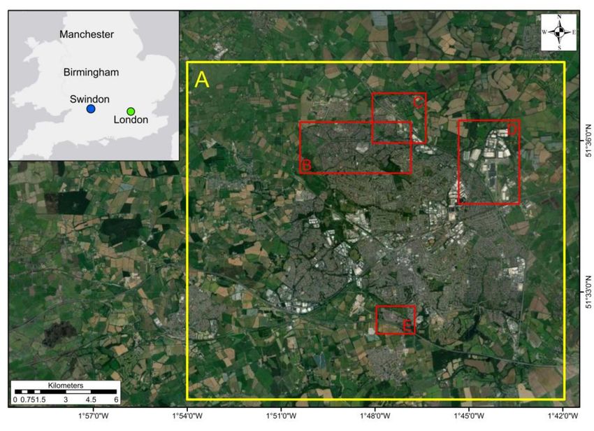
Remote Sens. 2021, 13, 3339                                                                                           2 of 22

                              proportion of the study area changes over time, as is often the case, then even highly
                              accurate classifications can lead to substantial error in the change estimates. Some of
                              this error may be mitigated by a process of temporal filtering. This method is applied at
                              the pixel level and identifies the change trajectory (or life-history) from multi-temporal
                              land cover classifications. Rule-based corrections are then made based on assumptions
                              of transition likelihood (e.g., assuming urban growth is irreversible) [7–9]. This process
                              may reduce misclassification error but only for those misclassifications identified by the
                              ruleset; other misclassifications which appear as allowed transition types may be missed.
                              Finally, real transitions can be erroneously removed when they are deemed to be unlikely;
                              therefore, bias may be introduced into the analysis. Pre-classification change detection
                              techniques have been developed in response to the problems of PCC. These approaches
                              use multitemporal, unclassified data to identify where changes take place and the nature
                              of the change that occurred [10]. Pre-classification methods are by their multitemporal
                              nature more complex than post-classification methods: even without land cover change,
                              spectral signatures will vary considerably in space and over time; the challenge, then, is to
                              identify within the highly variable data which variations indicate a land cover change [6].
                              Numerous pre-classification change detection methods exist, such as NDVI trajectory
                              analysis [11], NDVI differencing [12], time series break-point analysis [13], and continuous
                              change detection analysis [14].
                                   This paper builds on the method introduced by Zhu and Woodcock [14], which applies
                              harmonic analysis to the normalised difference vegetation index (NDVI), a widely used
                              vegetation index calculated from the red and near-infrared spectral bands [15]. A low level
                              or absence of vegetation is a defining characteristic of urban areas which therefore exhibit
                              low NDVI values and intra-annual (seasonal) variation [9]. Rural areas are characterised
                              by higher proportions of vegetation undergoing marked growth cycles, therefore exhibit-
                              ing either higher NDVI values or larger seasonal variations of NDVI [16]. Sufficiently
                              large deviations from established of NDVI temporal dynamics may be an indication of
                              change [12].
                                   The NDVI of a pixel fluctuates naturally over time both seasonally and through a
                              year-on-year trend. The signal can therefore be modelled using a harmonic analysis, e.g., a
                              sinusoidal function with a period of one year to reflect seasonal variation, and a linear
                              trend to reflect year-on-year growth [14,16]. Harmonic analysis is widely used for the
                              detection of cycles in data [17]. Theoretically, there is no limit to the number of sinusoidal
                              components to model a time series; pragmatically, however, researchers use only a few [18].
                                   Previously, Zhu and Woodcock [14], estimated a harmonic model for each pixel and
                              identified a land cover change where new observations deviated from the estimated model
                              beyond a given tolerance for three consecutive cloud-free observations. Zhu et al. [19]
                              applied a similar method with a lower threshold for identifying change, but a requirement
                              for a longer sustained deviation. In this article, we are concerned with change of land
                              cover due to urbanisation in an area prone to cloud cover and will expand on the methods
                              considering associated assumptions. We are assuming that land cover change is infrequent
                              and irreversible and will therefore not attempt to identify more than one change event
                              per pixel. We also intend to be robust under frequent cloud cover, which means that pixel
                              observations may be obtained at irregular time intervals. The proposed method is therefore
                              based on separately fitted sinusoidal functions for the period before and after a potential
                              change event. A change event is detected when the fit (root mean squared error, RMSE)
                              for the two separate models outperforms that of a single model for the whole period by
                              a given threshold. The timing of change for a pixel is determined by the best fit (lowest
                              RMSE) for the combined before and after models.
                                   This article presents the method and its application to a case study area in southern
                              England using the full time series of Landsat data from 1984 to 2018. Landsat data were
                              selected for this study despite their relatively coarse resolution (30 m pixels), which cannot
                              accurately outline many features in urban landscapes. They are used because of their
                              universal availability and their long historical archive; a long-time record is crucial for
Remote Sens. 2021, 13, 3339 3 of 22
analysis of urban change processes that have characteristic temporal scales in the order
of decades. The accuracy is assessed using a dense set of ground truth pixels and their
performance is compared to a PCC of existing UK land cover products.
2. Study Area
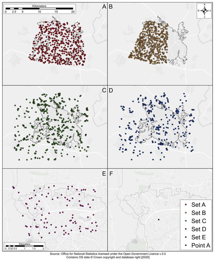
The study area consists of the town of Swindon and its surrounding area (Figure 1).
Swindon is in the south-west of England and has undergone substantial urban development
in the last century [20,21]. Swindon has a population of approximately 175,000 and has
undergone recent, rapid growth and has a history of flooding [22]. During the mid-20th
century, Swindon relied on railway-related activities yet by 1986 this was superseded by
the automotive, IT, and services sectors [23]. Swindon has received investment from Honda
which developed the South Marston industrial complex in 2001 [24]. This new source of
employment may have provided the catalyst for further suburban development in the
Hayden Wick area and facilitated a total population increase of 4.9% between 2001 and
2007 [23]. The town is surrounded by agricultural land and is not constrained by greenbelt
policies. The town has seen substantial impervious surface growth [25].
Figure 1. Location of Swindon in the UK relative to London. Yellow A: Study area. Red B: Haydon
Wick, C: Blunsdon Bypass, D: South Marston industrial complex, E: East Wichel.
3. Materials and Methods
3.1. Landsat Data
This study uses the Landsat archive [26], available through Google Earth Engine [27],
for the period from 1984 to 2018. This dataset includes images acquired by Landsat The-
matic Mapper (Landsat 5), Enhanced Thematic Mapper Plus (Landsat 7), and Operational
Land Imager (Landsat 8). This study used tier 1 surface reflectance data which have been
atmospherically corrected using the Landsat Ecosystem Disturbance Adaptive Processing
System (LEDAPS), and include a cloud, shadow, water, and snow mask identified using the
CFMask algorithm [28–31]. The dataset for the whole study area consists of 760 Landsat
images. Over half of all pixels were masked out due to the presence of clouds and shadows
as indicated by a pixel quality band generated by the CFMask algorithm [31]. Any pixel
in any image which was identified by the CFMask as being contaminated with clouds,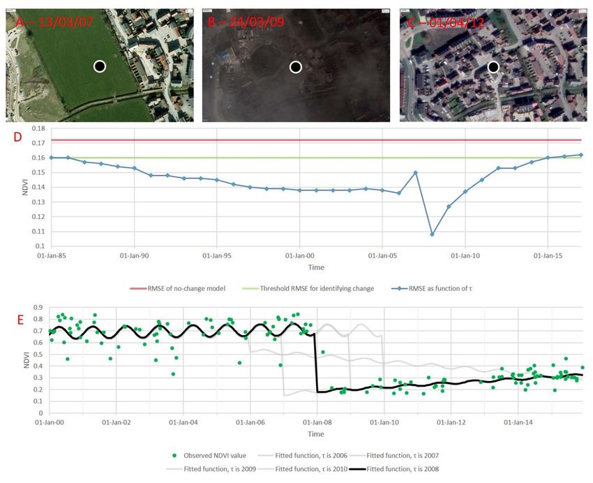
Remote Sens. 2021, 13, 3339                                                                                                4 of 22

                                shadow, water, or snow, was removed from the analysis; however, corresponding pixels in
                                other images remained in the analysis if they were identified as cloud-free. The red and
                                near-infrared bands, which have a spatial resolution of 30 m, were used to calculate the
                                NDVI [32]. In this study, no harmonisation between Landsat sensors was performed as
                                during preliminary analysis, the NDVI calculated from surface reflectance images was
                                observed to have a negligible impact on long-term average trends (the NDVI linear trend
                                and amplitude, calculated below).

                                3.2. Ground Truth Data
                                     Five sets of pixels were randomly and independently selected, prior to manual in-
                                terpretation using high-resolution imagery from Google Earth Pro [33]. Google Earth
                                images represent the highest resolution source of ground truth data available to this study;
                                whilst site visits would likely yield higher quality data, the retrospective nature of this
                                study made this impossible [34]. The availability of images for this area is not uniform,
                                whereby the western half of the study area has a denser coverage. The whole study area
                                is covered by images from 2002, 2003, 2005, 2012 and 2017 (Table 1). The high-resolution
                                images are of varying spatial resolution and quality, resulting in differences in ease of
                                interpretation. Georeferencing errors are generally small (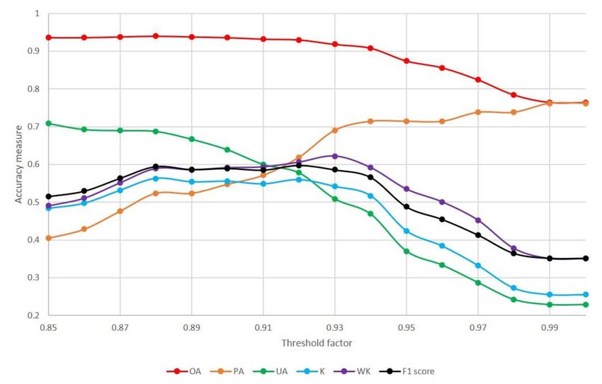
Remote Sens. 2021, 13, 3339                                                                                                  5 of 22

                              •    Set C consists of 500 pixels, randomly selected from those pixels that were classified
                                   as having change by the model. They were assessed for the period 1 January 2006–
                                   31 December 2014 and used for training the change classification stage (Figure 2C).
                              •    Set D consists of 300 pixels, randomly selected from those pixels that were classified
                                   as change by the model. They were assessed for the period 1 January 2006–31 Decem-
                                   ber 2014 and were used for accuracy assessment of the change classification stage
                                   (Figure 2D).
                              •    Set E consists of 100 pixels, randomly selected from the Haydon Wick area. Change
                                   was assessed from 1 January 2002–31 December 2014 and were used to test the dating
                                   capability of the model (time-of-change) (Figure 2E).
                              •    Point A (Figure 2F) was manually selected from Set B to demonstrate the methodology
                                   (Figure 3).

                              Figure 2. Location of the ground truth and accuracy assessment points used. (A) The 500 points used
                              to assess the threshold values. (B) The 500 points used in accuracy assessment of the model and PCC.
                              (C) The 500 training data points selected from the change class for classification. (D) The 300 points
                              used in accuracy assessment of the change classification. (E) The 100 points selected from the Haydon
                              Wick area to assess the accuracy of dating of change (selected from location B in Figure 1). (F) The
                              single point chosen from Set B to demonstrate the methodology (Figure 3).
Remote Sens. 2021, 13, 3339 6 of 22
Table 2. Land cover classes used in the study.
Abbreviation Defining Characteristics and Major Class
Land Cover Class Major Class
in Text Classification Criteria Abbreviation in Text
Sparsely built-up SBU A mix of buildings and vegetation Urban U
Dominated by buildings, vegetation
Densely built-up DBU Urban U
largely absent
No buildings or vegetation (e.g., car parks,
Bare ground BG Urban U
bare soil)
Vegetated VE Farmland or grass Vegetation V
Vegetated with minor Vegetated land with presence of small
VMS Vegetation V
structures structures, paths, water, shrubs, or trees
Figure 3. Illustration of method on a single pixel. (A–C) High-resolution images across the change occurrence, spot
indicating centre of pixel. (D) Goodness-of-fit as function of assumed time-of-change, threshold is h = 0.93. (E): NDVI trend
of observations, along with fitted functions. Black line corresponds to lowest RMSE, indicating the time-of-change.
Set A will be used to detect change from 2003 to 2012, sets B, C, and D will detect
change from 2006 to 2015. Finally set E will detect change from 2002 to 2015. Sets A and B
were randomly selected from across Swindon and are therefore spatially balanced. SetsRemote Sens. 2021, 13, 3339 7 of 22
C and D were randomly selected from those pixels identified as change in the validation
map (see below). Set E was oversampled in an area of substantial urban growth to test the
method’s dating capability and is therefore not spatially balanced.
Olofsson et al. [34] discuss issues with the manual classification of ground truth pixels.
To address these issues, all the classifications, timings, and justifications are included in the
Supplementary Data (Points).
3.3. Centre for Ecology and Hydrology Land Cover Products
The PCC used the UK’s Land Cover Map of 2007 and 2015: LCM 2007 and LCM
2015 [35,36]. These datasets are primarily derived from Landsat data, although further
knowledge-based enhancements using ancillary data were used in their creation. LCM
2007 uses images ranging from 2 September 2005 to 18 July 2008, and LCM 2015 images
from 1 January 2014 to 10 December 2015 [35,37]. An overall accuracy of 83% is reported
for LCM 2007 [35]. The maps were produced using a polygon-based classification where
homogenous polygons were identified (with a minimum mapping unit of 0.5 ha), then clas-
sified by land cover type. It should be noted that the documentation states unambiguously
that the maps must not be used for change assessment [35]; however, in practice this is
likely the only avenue available for analysts relying on secondary data.
The classes are not uniform between the two maps; therefore, aggregation of certain
classes was performed. Several classes were absent from the study area and were disre-
garded, these were: acid grass, fen and marsh, bog, montane, saltwater, supra-littoral rock,
supra-littoral sediment, littoral rock, littoral sediment, and salt marsh. Certain classes,
namely broadleaf, conifer, horticultural and arable, inland rock, freshwater, urban, and
sub-urban were comparable between LCM products. The heather class was absent in
2007 and present in 2015; therefore, the LCM broad habitat of Dwarf Shrub was used to
aggregate heather and heather grassland together (the latter being present in both years).
Finally, rough grassland was removed in the production of LCM 2015, and therefore grass
landcover classes were aggregated into the broad habitat of “grass”, these being: improved,
rough, neutral, and calcareous grassland.
3.4. Methods
3.4.1. Method Outline
NDVI was first calculated for all cloud-free pixels across all images. NDVI was
chosen as the single metric for change detection; as a vegetation index it is subject to
periodic cycles and is a (counter) indication of urbanisation. Other studies have successfully
detected land cover changes using solely NDVI and derived statistics [11,38], particularly
sinusoidal function change detection methods [18,39]. The method of change detection and
classification has two stages. The first stage is a binary change detection which identifies
pixels where a change occurs and predicts the timing of the change event. The second stage
uses a random forest to classify the type of change that occurred in the change pixels. The
supervised random forest classifier was selected due to its non-parametric nature, potential
for high accuracy results [10], and wide use within GEE based studies (e.g., [11,40,41]). The
accuracy of the change detection, the type of change, and the time-of-change were assessed
separately. The change detection map was then compared to that of a PCC assessment
using LCM 2007 and LCM 2015.
3.4.2. Change Detection
The change detection algorithm is applied to each individual pixel in the study area.
Two models are fitted to the NDVI time series of the pixel: the change model and the
no-change model. The change model is accepted if its fit is better than that of the no-change
model by a given threshold factor. The threshold is necessary, because the change model has
additional degrees of freedom and will always have a better fit than the no-change model.Remote Sens. 2021, 13, 3339 8 of 22
The no-change model fits a sinusoidal function with a period of one year, superimposed
onto a linear trend, to the NDVI signal [42]:
NDV Ino change (t) = a sin(2πt) + b cos(2πt) + c t + d (1)
where NDV Ino change (t) is the predicted value of NDVI if no-change is assumed; t is time
in years; and a, b, c, and d are estimated coefficients. c is the slope of the linear trend of
mean NDVI and d its intercept. The parameters a and b describe the oscillation around the
mean and are more readily√ interpreted when transformed. Note that a sin( x ) + b cos( x ) =
Rcos( x − α), with R = a2 + b2 and tan(α) = b/a, and hence the amplitude of the annual
oscillation is R and its phase is determined by α.
The change model fits the same model to the NDVI signal but allows a structural break
and a different set of coefficients before and after the break:
t < τ : a0 sin(2πt) + b0 cos(2πt) + c0 t + d0
NDV Ichange (t) = (2)
t ≥ τ : a1 sin(2πt) + b1 cos(2πt) + c1 t + d1
where NDV Ino change (t) is the predicted value of NDVI if change is assumed; and a0 , b0 ,
c0 , d0 , a1 , b1 , c1 , and d1 are estimated coefficients. τ, the time-of-change, is also estimated.
The analysis was implemented in Google Earth Engine and made use of a built-in tool for
linear regression to estimate the a, b, c and d coefficients for both the change, and no-change
model. These coefficients are estimated using the iteratively reweighted ordinary least
squares regression using the Google Earth Engine Talwar cost function [43]. This technique
is more robust to outliers in the data than ordinary least squares regression and is intended
to compensate for missed cloudy pixels. A similar reweighting was performed by Zhu,
Woodcock and Olofsson [44]. The time-of-change, τ, in the change model is estimated by
iterating over its domain in increments of one year and retaining the value with best fit
(RMSE). Five iterations are shown in Figure 3E.
The goodness-of-fit of both the change model and the no-change model is calculated
as RMSE and the change model is accepted if it outperforms the no-change model by a
given factor: h i
change = RMSEchange ≤ h × RMSEno−change (3)
where change is a binary value indicating if change is detected in a pixel Figure 3D. h is
a threshold value (0 < h ≤ 1) that is not known a priori. We use our first ground truth
dataset (Set A) to find the optimal value of h based on the weighted kappa statistic [45],
attaching partial agreement between the change and partial-change class, and total agreement
between partial-change and no-change. We applied the method with all h values between
0.85 and 1 in increments of 0.01.
The model is estimated for Landsat data from 1984 to 2018; for the calibration of the
threshold factor (h) only changes over the period 2003–2012 are detected, this threshold is
then used to detect changes for the period 2006–2015.
3.4.3. Accuracy Assessment of Change Detection
The threshold parameter h is the only parameter that depends on training with ground
truth data (Set A for 2003–2012). For the validation, the model is applied to another period
(2006–2015) and assessed against a second sample of ground truth data (Set B) to coincide
with the images used to produce the LCM 2007 and 2015, rather than their nominal dates.
The ground truth data were classified using the classes change, no change, and partial-
change, whereas the model detects just change and no-change. Partial-change defines any
noticeable structural reconfiguration covering less than 50% of the area of a pixel takes
place. Most comparison methods (overall (OA) and user’s accuracy (UA), kappa statistic
(K), and F1 score) require identical classes in the model and ground truth data; for these,
partial-change was counted as no-change, and, conversely, producer’s accuracy (PA) was
calculated separately for the no-change and partial-change classes, to provide better insightRemote Sens. 2021, 13, 3339 9 of 22
into the nature of disagreements. This results in a 3 × 2 confusion matrix, rather than
the more conventional tables 2 × 2 in a binary classification. The weighted kappa (WK)
method [45] allows partial agreement between classes, and here we considered the partial-
change class as fully in agreement with no-change and 50% in agreement with change. Based
on these classifications we calculated the goodness-of-fit measures set out in Congalton
and Green [46], including UA and (unbiased) PA, (unbiased) OA, and K. F1 score (or F
measure) was calculated to quantify the balance between producer’s and user’s accuracy
of the change class [47]. The widespread use of the kappa statistic in remote sensing and
land use/cover modelling has attracted substantial criticism [48]; therefore, we present
results alongside contingency tables and other accuracy metrics that together provide a
fuller assessment of accuracy. Where a single summary measure is required, kappa remains
a useful metric as it accounts for the uneven marginal distribution over the classes. In the
current case, where there is a very low incidence of change compared to no-change, this is
a necessity.
3.4.4. Accuracy Assessment of the Time-of-Change
Of the 500 sampled points of Set B, only a small fraction of pixels changed from rural to
urban. Since our primary objective was to detect urban growth, we oversampled a further
100 randomly selected points (Set E) in the Haydon Wick area (Figure 1), where considerable
urban growth took place over the study period. This sample was used to gain insight
into the temporal accuracy of the change detection. These pixels were manually assessed
for change using the high-resolution imagery for the period of 2002–2015. Due to the
intermittent availability of high-resolution imagery, the timing of change was determined
as the period between the timestamp of the last pre-change and first post-change high-
resolution image—typically a period of a few years. Transitionary land covers (most
frequently bare ground or an impervious surface worksite) were counted as partial-change
if they were the first instance of change in high resolution imagery.
3.4.5. Classification of Transition Types
Change pixels were then classified into the type of transition that occurred. This
classification is based on the parameters of the estimated model, i.e., a0 , b0 , c0 , d0, a1 , b1 ,
c1 , d1 , and τ. These parameters have limited physical meaning and therefore four more
pertinent parameters are derived from the original nine:
q
R0 = a20 + b02 (4)
q
R1 = a21 + b12 (5)
M0 = co τ + do (6)
M1 = c1 τ + d1 (7)
where R0 and R1 are the amplitude of the estimated NDVI trend before and after the
time-of-change, respectively. M0 and M1 are the mean of the estimated NDVI trend just
before and after the time-of-change, respectively.
A total of 500 pixels were randomly chosen from the change class identified in
Section 3.4.2, over a larger area than previous stages to encompass rural change surround-
ing Swindon rather than focusing solely on the urban environment (Set C). Change was
manually classified into four major class transitions: vegetation to vegetation (V–V), vege-
tation to urban (V–U), urban to urban (U–U), and urban to vegetation (U–V). Vegetation
consists of the manual classification of VE or VMS, and urban consists of the manual classi-
fication of BG, SBU, and DBU (Table 2). Due to the small proportion of U–V (five pixels),
pixels in this class were removed from analysis and only the first three classes were used,
as is more commonly carried out [38,39]. A further three pixels were manually classified as
water and were removed, leaving 492 pixels as ground truth data for the classifier.Remote Sens. 2021, 13, 3339 10 of 22
False positives were included in the training data as the aim of this section was to
test the accuracy of the pre- and post-change land cover classification, not the change
detection capability of the algorithm. Our study is particularly interested in rural to urban
transitions; therefore, intra-class transitions are of lesser interest. Once ground truth data
were manually classified, box plots for the remaining pixels were calculated to explore the
usability of the parameters for classification. This dataset of pixels was used as training
data for a random forest classification using all four parameters (Equations (4)–(7)). The
random forest was implemented in the Google Earth Engine using its default settings
√
(namely the number of variables per split ( (4)), minimum leaf population (1), and bag
Fraction (0.5)). A total of 300 trees were used, as previous work has shown this to offer a
reasonable compromise between accuracy and speed in the Google Earth Engine [41].
3.4.6. Accuracy Assessment of Transition Types
The accuracy of the classification was tested using a further 300 randomly selected
pixels from within the change class. Similarly, false positive change pixels were included
to independently test the classification of from–to classifications. Two examples of urban
to vegetation were found, and a single pixel dominated by water. These were removed,
leaving 297 pixels for accuracy assessment.
4. Results
4.1. Change Detection
The method estimates for every pixel both a model for change and a model for no-
change. The change model is accepted if the RMSE is smaller by a given threshold factor (h)
than the no-change model. We tested all values of h between 0.85 and 1 in steps of 0.01. The
selection of the appropriate threshold was based on the WK. The impact on the accuracy
measures over the training period is shown in Figure 4. The threshold parameter (h) most
strongly affects the UA and PA. F1 score is approximately equal for all thresholds between
0.88 and 0.93, with values decreasing outside this range. Increasing h means that more true
changes are identified, increasing the PA, but also more no-change pixels are identified as
having undergone change, decreasing the UA.
Figure 4. PA and UA of the change class; OA and WK comparison for all values of h. Note that for
UA, OA, K, and F1 score, partial-change is counted as no-change. For WK, partial-change is in half
agreement with change, and full agreement with no-change.Remote Sens. 2021, 13, 3339 11 of 22
The weighted kappa coefficient (0.622) was used to determine the appropriate thresh-
old value of 0.93. The corresponding overall accuracy is 91.8%, the user’s accuracy is 50.9%
and the producer’s accuracy is 69.0%.
The trained model was then applied to the validation period 2006–2015 and assessed
against an independent sample of ground truth data (Set B). The results give an assessment
of where and when a transition in land cover occurred (Figure 5). The results indicate
substantial contiguous areas of land cover change in the four areas where major urban
development took place over the study period, these are suburban expansion in the Haydon
Wick area and East Wichel, minor expansion of the South Marston industrial complex post
initial construction, and construction of the new Blunsdon bypass (initial work began with
archaeological excavations in 2006 [49]).
Figure 5. Land over change map produced for the period of 2006–2015.
Changes outside of these known areas of urban growth are found within both the
urban and rural environments. In the urban environment, identified changes are mainly in
small patches (groups of contiguous pixels that change at the same time) or isolated pixels,
whereas in the rural areas change occurs in predominantly large patches (Figure 5).
The accuracy of the validation change detection was assessed against 500 manually
examined ground truth points (Set B) and the results are cross tabulated in a contingency
table (Table 3). An overall accuracy of 91.2% for correctly identified change/no-change was
found. The kappa index of agreement is 0.475 and weighted kappa is 0.486 (Table 4).Remote Sens. 2021, 13, 3339 12 of 22
Table 3. Contingency table of model and ground truth data for the period of 2006–2015.
Ground Truth
No-Change Total
Change
Partial-Change No-Change
Change 24 6 23 53
Model
No-change 15 69 363 447
Total 39 75 386 500
Table 4. Accuracy measures and associated confidence intervals. The model shows three sets of statistics corresponding
to three sets of analysis and three sets of accuracy assessment data (Sets A, B, and E). The training period are the values
from the selected 0.93 threshold iteration. The validation model is directly comparable to the PCC as both use the same
sample set (Set B). Time-of-change analysis was performed over the oversampled area of Haydon Wick for the increased
time period of 2002–2015. Kappa values are presented with estimations of large sample variance using Delta method [46].
Note that for UA, OA, K, and F1 score, partial-change is counted as no-change. For WK, partial-change is in half agreement
with change, and full agreement with no-change.
Model
Metric PCC
Training Period Validation Period Time-of-Change
OA (%) 91.8 91.2 86.0 72.6
K 0.542 ± 0.00835 0.475 ± 0.00678 0.720 ± 0.00616 0.181 ± 0.00177
K significant above 1.96 5.93 5.76 9.17 4.30
WK 0.622 0.486 0.762 0.198
PA of change (%) 69.0 61.5 87.2 69.2
PA of no-change (%) 97.6 94.0 94.7 73.8
UA of change (%) 50.9 ± 4.47 45.3 ± 4.45 83.7 ± 7.39 17.8 ± 3.42
UA of no-change (%) 97.1 ± 1.51 96.6 ± 1.61 88.2 ± 6.44 96.6 ± 16.3
Unbiased PA of change (%) 66.4 ± 13.6 61.7 ± 13.9 88.1 ± 8.31 71.4 ± 13.6
Unbiased OA (%) 92.3 ± 5.46 91.1 ± 4.72 85.9 ± 9.85 70.8 ± 4.31
F1 score of change 58.56 52.2 85.4 28.3
Using the method outlined in Congalton and Green [46], confidence intervals of
overall, producer’s and user’s accuracy of change, and large sample variance of kappa
were calculated. For Congalton and Green [46], confidence intervals require the use of
unbiased producer’s and overall accuracy calculated from map marginal proportions not
derived from the error matrix; however, this normalisation results in only a small variation
of accuracy measure.
4.2. Post-Classification Change Detection
The PCC of the LCM 2007 and LCM 2015 identifies considerably more change than
our method (Figure 6). The confusion matrix of the PCC (Table 5) results in an increased
producer’s accuracy of change, yet user’s accuracy is greatly decreased compared to our
analysis (Table 4). The great disparity between user’s and producer’s accuracy of change is
reflected by a low F1 score (Table 4). This is also reflected in a poorer kappa and overall
accuracy metrics due to an increased false positive rate.Remote Sens. 2021, 13, 3339 13 of 22
Figure 6. Comparison of the harmonic model output with a PCC land cover map from [35,36].
Uncoloured areas were detected as having undergone no-change in both methods. Grey line represents
outline of urban extent as of 2015.
Table 5. Confusion matrix of the PCC of LCM2007 and LCM 2015 with 500 ground truth pixels.
Ground Truth
No-Change Total
Change
Partial-Change No-Change
Change 27 24 101 152
PCC
No-change 12 51 285 348
Total 39 75 386 500
By comparing the results of Set B between the model and the PCC it is revealed that
the methods agree with change in a small proportion of pixels (Table 6). The kappa statistic
between the two methods is 0.138, indicating almost random agreement.
4.3. Type of Change
The type of change observed in the ground truth data for Set B, and the number of
true positives and false negatives is shown in Table 7. The most numerous changes were
conversions of bare ground to sparsely built-up, vegetated to bare ground, and vegetated
to sparsely built-up.Remote Sens. 2021, 13, 3339 14 of 22
Table 6. Agreement between our model and PCC. Kappa statistic = 0.138. Note, these are not
necessarily correctly identified, merely agreement between the two methods.
PCC
Total Agreement
Change No-Change
Change 28 25 53 52.8%
Model
No-change 124 323 447 72.3%
Total 152 348 500
Agreement 18.4% 92.8% 70.2%
Table 7. Manual classification of pixels identified as change. Columns show final land cover, rows
show original land cover. First number indicates correctly identified change (true positives); second
value (in brackets) gives the number of false negatives of the change class.
Final Land Cover
VE VMS SBU BG DBU
VE 0 (0) 1 (1) 6 (1) 5 (0) 0 (0)
VMS 0 (0) 1 (0) 1 (0) 2 (1) 0 (0)
Starting Land Cover SBU 0 (0) 0 (1) 0 (2) 0 (1) 1 (0)
BG 0 (0) 0 (0) 4 (5) 2 (1) 1 (1)
DBU 0 (0) 0 (0) 0 (0) 0 (0) 0 (1)
4.4. Time-of-Change
A further 100 pixels (Set E) were analysed in an area that saw substantial rural to urban
change over the time-period of 2002–2015 to assess the temporal accuracy of our method.
Of these, 47 pixels underwent land cover change, with the model correctly identifying
41. In addition, the model identified six pixels in the partial-change category as change; to
assess what the model is detecting when it detects partial-change, these were included in
the analysis (for a total of 47 pixels). Table 4 shows that the change detection rate in an area
where there is considerably more change is vastly improved.
In the time-of-change accuracy assessment ground truth data, the period within which
change occurred was between the time of the last image before the change and the first
image after the change. For 42 (89.4%) pixels, the estimated time-of-change was within the
period identified in the ground truth data (Figure 7). Of the five incorrectly dated pixels,
the model determined change occurred more recently in four instances, with a maximum
difference of five years. The middle value of the period of potential change is shown by the
yellow line in Figure 7. The average time-period of potential change was 2.7 years with a
standard deviation of 1.3 years. The model correctly dated all partial-change pixels that it
detected as undergoing change.
4.5. Classification of Transition Types
Before applying the random forest classification, we explored the distribution of the
parameters over the three transition types to explore the separability based on this input
data and classification scheme. The results show reasonable separation and are in line with
the normal expectation that rural areas experience greater amplitudes and mean NDVI
levels (Figure 8).Remote Sens. 2021, 13, 3339 15 of 22
Figure 7. Bars show range of high-resolution images denoting the period of possible change. Grey bars show change,
black bars show partial-change. Yellow line denotes the middle period of the high-resolution image range. Abbreviations
correspond to Table 2.
Figure 8. Box plots of the parameters of the training data (Set C) used to classify the type of change.
(A) Mean value of the NDVI trend before and after change, (B) amplitude before and after change.Remote Sens. 2021, 13, 3339 16 of 22
The final step of analysis was to classify the resulting change layer to understand rural
to urban change, and this follows herein.
Ground truth data were gathered from 500 pixels and manually classified into veg-
etation to vegetation (222 pixels), vegetation to urban (107 pixels), and urban to urban
(163 pixels) change. Five pixels undergoing urban to rural change, and three pixels covering
mostly water, were excluded, leaving 492 pixels as training data. A random forest classifier
was used to classify the validation map. The resultant layer of transitions (Figure 9) shows
a clear urban gradient. The centre is dominated by urban to urban transitions, at the
urban periphery rural to urban is the main transition type and in the rural areas, rural to
rural transitions are most common. Applying the classification of growth patterns from
Xu et al. [50], it appears that there is a degree of infill and leapfrogging, but the major
pattern of growth is edge expansion.
Figure 9. Classified change map produced using a random forest classifier. Grey line represents
urban extent as of 2015 and may be used to qualitatively assign urban change to edge expansion,
infill, and leapfrog type growth.
For validation a further 300 randomly selected pixels from within the change class of
the validation model were chosen Those which underwent urban to vegetation (two pixels)
transitions and a single pixel which was dominated by water were removed, leaving
297 pixels for accuracy assessment.
The key statistics based of the confusion matrix (Table 8) have an overall accuracy
of 83.2% and a kappa statistic of 0.724. The lowest accuracies (both PA and UA) were
observed in the V–U class.Remote Sens. 2021, 13, 3339 17 of 22
Table 8. Confusion matrix of transition types for 297 pixels accurately classified as changed.
Ground Truth
Total UA
V–V V–U U–U
V–V 133 17 5 155 85.8
Classification V–U 13 34 7 54 63.0
U–U 4 4 80 88 90.9
Total 150 55 92 297
PA 88.7 61.2 87.0 83.2
4.6. Number of Clouds per-Pixel
The number of observations per-pixel ranged between 697 and 731, as not all images
covered the entire study area. Per-pixel minimum and maximum cloud-free observations
were: 72 (a highly mixed SBU pixel) and 343 (a pure VE pixel), respectively. These two
pixels were investigated individually and were both correctly identified as undergoing
no-change.
The cloud-free coverage for all pixels in Set B was tabulated by both model and ground
truth classification (Table 9). For pixels within this set, the minimum cloud-free coverage for
a pixel was 158 (21.9%), and the maximum was 332 (45.8%). There is no obvious correlation
between cloud-free coverage and change detection (Table 9).
Table 9. The average percentage of cloud-free pixels in Set B by change classification.
Ground Truth
No-Change
Change
Partial-Change No-Change
Change 41.0 41.8 43.2
Model
No-change 41.8 42.0 42.2
Out of the 500 pixels of Set B, the 50 pixels with the highest number of cloud-free
pixels, and the lowest 50 pixels were inspected to determine any correlation to land cover
class. Of the lowest 50 pixels, only 10 involved rural classes (either change to for from V, or
stable V); conversely, of the highest 50 pixels, 35 involve the V class. DBU is absent from
the top 50 pixels, and VE is absent from the lowest 50 pixels.
5. Discussion
5.1. Detection, PCC, and Type, and Timing of Change
The manually classified class of partial-change is of particular interest. This class
mostly coincides with no-change in the automated procedure, but holds 20.7% of the pixels
misclassified as change, even though it only contains 16.3% of all no-change pixels (Table 3).
Nominally, a UA of 45.3% may be considered low; however, the model comfortably
outperforms the common practice of PCC (UA = 17.3%). The PCC method used information
from additional Landsat bands and ancillary data not used in this study. As a proof-of-
concept, this demonstrates the viability of our method. Future studies may expand our
method to incorporate other available information to improve accuracy and apply the
method to a wider scale.
The relatively large confidence intervals on the PA of each model iteration may be
attributed to the considerable proportional difference between the area (or total number
of pixels) of change vs. no-change (including partial-change) (Table 4). In the threshold
and validation time periods, the ratio of change vs. no-change area is approximately 1:11.
Similarly, due to the small area of change relative to no-change, the UA will be negatively
impacted by a moderate proportion of error in the non-changing land (false positives). InRemote Sens. 2021, 13, 3339 18 of 22
the time-of-change analysis, however, the proportion was approximately 50:50. This run
yields the lowest confidence interval on the PA and highest UA of change, suggesting a
stratified random sample should be recommended for future change detection research
and would likely increase the UA of this study. The drastically improved UA (relative
to the training and validation runs) of the time-of-change analysis, however, may be an
artefact: as most observed changes were from a rural to an urban land cover, these changes
undergo large drops in NDVI (Figure 8A), which our model is optimised to detect. In the
time-of-change analysis, a slight majority (51.1%) of correctly identified pixels are above
the middle of the date range (Figure 7), suggesting a robust method of dating change.
The disparity between the PA and UA of the PCC is clearly demonstrated via the
lowest F1 score of any change detection (Table 4). The greatly increased PA comes at the
expense of a reduced UA, which is reflected in other statistics, particularly the K. This is in
line with the theoretical expectation that PCC overestimates changes as classification errors
in either layer are registered as change [6] and is a known issue with the method. The
PCC detects the most change, reflected in Table 6 and Figure 6. In principle, however, PCC
analysis should find fewer changed pixels, as it excludes changes within a land cover class.
Furthermore, the LCM uses a minimum mappable unit and, hence, fine-grained changes
are less likely to be registered.
Table 7 shows that the most commonly detected and occurring changes were BG–SBU,
VE–BG, and VE–SBU, clearly demonstrating the large proportion of urban growth occurring
in Swindon during the study period. These changes reflect the suburban expansion via
the conversion of rural fields to either worksites or constructed housing, or the completion
of worksites to housing. The high accuracy of detection of conversions of VE to either BG
or SBU likely reflects the dramatic change in NDVI values which would accompany this
type of change (Figure 8A). Similarly, the poor detection of BG to SBU may be due to the
similarity of NDVI values between these classes.
The model most frequently confuses vegetation to urban with vegetation to vegetation;
this may be due to the relative greenness of some urban areas, as indicated by Figure 8,
which shows some overlap between these two classes. Figure 8 suggests that the value of
the mean NDVI trend before and after change may be a better predictor of transition type
than amplitude due to the lack of overlap of the boxes of the plots. To improve change
detection and classification accuracy, the inclusion of other vegetation indices is an avenue
for further research. This can be achieved by the substitution of NDVI for other indices
into Equations (1) and (2).
5.2. Impact of Landsat Archive
This methodology uses the entire Landsat 5, 7, and 8 archive up to 2018 to detect
change for the period of 2006–2015. This period of analysis was chosen to facilitate com-
parison with the LCM products and coincide with the availability of the high-resolution
imagery used as ground truth data. This model requires at least one year prior to and after
the period of change for this to be detected. Zhu and Woodcock [14] note that this initialisa-
tion period can impact the outcome of the change detection algorithm. This may manifest
in two ways: firstly, the method is limited to detecting one instance of change per pixel;
therefore, change occurring outside of the period of change detection can mask change in
the period of analysis. Multiple changes in the same location are unlikely; however, they
are entirely possible. Urban growth is typically unidirectional; therefore, multiple changes
are unlikely. The purpose of our study was to detect urban growth; therefore, the detection
of a single change is a reasonable assumption; however, this may not be universally true.
Only a single pixel in all those analysed underwent two land cover changes in the period
between 2002 and 2015 (excluding transitionary land cover types such as worksites); how-
ever, partial-change was often associated with longer-term incremental changes totallingRemote Sens. 2021, 13, 3339 19 of 22
change. This may not be the case, as the considerable lead-in period allows for large
fluctuations in the bounded NDVI value (as NDVI cannot vary outside of −1–1), which
may not be accurately quantified by the linear component of a single sinusoidal function.
Any non-zero NDVI trend must at some point change, as NDVI cannot increase or decrease
ad infinitum. Therefore, the lead-in period may swamp the analysis and cause an incorrect
estimation of τ, as the model may find this yields a lower RMSE than the correct time-
of-change, leading to an incorrect change detection. Finally, the considerable mismatch
between the lead-in and -out length may have impacts on the change detection accuracies
that were not explored. The choice of these dates was constrained by the availability of
ground truth data, and it is postulated that change detection would be most accurate when
these periods were approximately equal. The length of the lead-in and -out period, and the
impact on change detection were not investigated and is a subject for future research.
5.3. Computation Time
Computationally, the most time-consuming step was the linear regression, estimation
parameters of Equation (2). Note that this step requires multiple linear regressions for
each pixel. This was performed on GEE cloud servers and took approximately 24 h. The
implementation of Equation (3) and the random forest classification took less than 10 min.
As a pixel-based algorithm, the computation time is expected to vary proportionally with
the number of pixels.
5.4. Impact of Changing Spatial Resolution
The 30 m resolution of Landsat is well suited to the detection of housing unit con-
struction but fails to adequately capture finer resolution changes, such as small increases in
paved surface in gardens. Increasing the spatial resolution of the sensor (such as by using
Sentinel 2) should not impact the accuracy of change detection in areas where the change is
larger than the Landsat pixel size, but will aid the detection of smaller changes, that would
be classified as partial-change at the Landsat resolution but complete change at the Sentinel
2 resolution.
Theoretically, this method requires only a single year of time series data before and
after the change detection period. However, it is expected to be more accurate and advan-
tageous than conventional pair date comparisons for longer periods, such as those of the
Landsat archive. However, the ideal time series length is subject to further research.
5.5. Impact of the Number of Clouds on Change Detection Accuracy
The percentage of cloud-free pixels appears to be independent of classification accu-
racy (Table 9). We therefore find that in the current study, sufficient cloud-free images were
available to not impede or bias the detection of change using this method. No testing was
undertaken to relate the accuracy of the method to the number and temporal distribution
of cloud-free observations. This can be addressed in the future by randomly deleting
observations and applying the method.
6. Conclusions
This study investigated the use of structural break detection in harmonic analysis to
detect and classify land cover change in the context of urban growth. An advantage of the
method is that it is based on the detection of a change of trend that is manifested over a
period. Hence, it is less sensitive to noisy and missing data, for instance due to cloud cover
and shadows, as is prevalent in the case study area. To detect change in any year, the model
requires a lead-in and -out period, therefore limiting usability in creating current maps.
Further work may assess the feasibility of smaller time units, such as six months. The case
study considered changes occurring between 2006 and 2015 but used the full archive from
1984 to 2018.
The method clearly outperforms PCC, even for a land cover product that is in many
senses superior to our approach; unlike the LCMs, we only considered temporal variationRemote Sens. 2021, 13, 3339 20 of 22
in NDVI and did not make use of ancillary data. We therefore consider the application a
successful proof of concept. In particular, the proposed method does not suffer from the
considerable bias toward detecting change of PCC and provides an accurate estimation
of the time-of-change. Notwithstanding, there is substantial scope for improvement: the
detection of changed pixels has a user’s accuracy of 45.3 ± 4.45%, and a classification user’s
accuracy of rural to urban of 63.0%.
Further refinements to improve the accuracy, aside from incorporating data from
other sources, are possible. One avenue is to make fuller use of the spectral information in
the Landsat archives, beyond NDVI. Other options are to expand the model to allow for
multiple change events per pixel over time, particularly to detect transitional land cover
classes, and to integrate changes in the fit between model and data in the identification of
structural breaks. Finally, the method may be applied to other image collections with the
capability of calculating NDVI such as Sentinel 2.
Supplementary Materials: The following are available online at https://www.mdpi.com/article/10
.3390/rs13163339/s1, Tables: Points.
Author Contributions: Conceptualization, M.N.L., B.M.-C. and A.H.-Z.; methodology, M.N.L.,
B.M.-C. and A.H.-Z.; software, M.N.L.; validation, M.N.L.; formal analysis, M.N.L.; investigation,
M.N.L.; writing—original draft preparation, M.N.L., B.M.-C. and A.H.-Z.; writing—review and
editing, M.N.L., B.M.-C. and A.H.-Z.; visualization, M.N.L.; supervision, B.M.-C. and A.H.-Z.; project
administration, M.N.L.; funding acquisition, B.M.-C. and A.H.-Z. All authors have read and agreed
to the published version of the manuscript.
Funding: This research was funded by SCENARIO NERC Doctoral Training Partnership grant
NE/L002566/1.
Institutional Review Board Statement: Not applicable.
Informed Consent Statement: Not applicable.
Data Availability Statement: For analysis, we used publicly available tools: Google Earth Engine
and publicly available Landsat 5, 7, and 8 imagery. The Google Earth Engine scripts images are
available at https://github.com/MNLawton/Time-Series-Harmonic-Analysis-Swindon (accessed
on 30 July 2021) All points assessed in this study (A-E) may be found in the same location. Further
requests should be made to the corresponding author (MNL).
Acknowledgments: The authors would like to thank the SCENARIO NERC Doctoral Training
Partnership for funding this PhD project which facilitated this research.
Conflicts of Interest: The authors declare no conflict of interest.
References
1. Population Division, Department of Economic and Social Affairs, United Nations. World Urbanization Prospects: The 2018 Revision;
United Nations: New York, NY, USA, 2019.
2. Herold, M.; Goldstein, N.C.; Clarke, K.C. The Spatiotemporal Form of Urban Growth: Measurement, Analysis and Modeling.
Remote Sens. Environ. 2003, 86, 286–302. [CrossRef]
3. Olofsson, P.; Foody, G.M.; Stehman, S.V.; Woodcock, C.E. Making Better Use of Accuracy Data in Land Change Studies: Estimating
Accuracy and Area and Quantifying Uncertainty Using Stratified Estimation. Remote Sens. Environ. 2013, 129, 122–131. [CrossRef]
4. Grinblat, Y.; Gilichinsky, M.; Benenson, I. Cellular Automata Modeling of Land-Use/Land-Cover Dynamics: Questioning the
Reliability of Data Sources and Classification Methods. Ann. Am. Assoc. Geogr. 2016, 106, 1299–1320. [CrossRef]
5. Mas, J.F.; Gao, Y.; Pacheco, J.A.N. Sensitivity of Landscape Pattern Metrics to Classification Approaches. For. Ecol. Manag. 2010,
259, 1215–1224. [CrossRef]
6. Zhu, Z. Change Detection Using Landsat Time Series: A Review of Frequencies, Preprocessing, Algorithms, and Applications.
ISPRS J. Photogramm. Remote Sens. 2017, 130, 370–384. [CrossRef]
7. Lark, T.J.; Salmon, J.M.; Gibbs, H.K. Cropland Expansion Outpaces Agricultural and Biofuel Policies in the United States.
Environ. Res. Lett. 2015, 10, 044003. [CrossRef]
8. Liu, H.; Zhou, Q. Accuracy Analysis of Remote Sensing Change Detection by Rule-Based Rationality Evaluation with Post-
Classification Comparison. Int. J. Remote Sens. 2004, 25, 1037–1050. [CrossRef]
9. Nguyen, L.H.; Joshi, D.R.; Henebry, G.M. Improved Change Detection with Trajectory-Based Approach: Application to Quantify
Cropland Expansion in South Dakota. Land 2019, 8, 57. [CrossRef]Remote Sens. 2021, 13, 3339 21 of 22
10. Rodriguez-Galiano, V.F.F.; Ghimire, B.; Rogan, J.; Chica-Olmo, M.; Rigol-Sanchez, J.P.P. An Assessment of the Effectiveness of a
Random Forest Classifier for Land-Cover Classification. ISPRS J. Photogramm. Remote Sens. 2012, 67, 93–104. [CrossRef]
11. Huang, H.; Chen, Y.; Clinton, N.; Wang, J.; Wang, X.; Liu, C.; Gong, P.; Yang, J.; Bai, Y.; Zheng, Y.; et al. Mapping Major Land Cover
Dynamics in Beijing Using All Landsat Images in Google Earth Engine. Remote Sens. Environ. 2017, 202, 166–176. [CrossRef]
12. Masek, J.G.; Lindsay, F.E.; Goward, S.N. Dynamics of Urban Growth in the Washington DC Metropolitan Area, 1973-1996, from
Landsat Observations. Int. J. Remote Sens. 2000, 21, 3473–3486. [CrossRef]
13. Hermosilla, T.; Wulder, M.A.; White, J.C.; Coops, N.C.; Hobart, G.W. Regional Detection, Characterization, and Attribution of
Annual Forest Change from 1984 to 2012 Using Landsat-Derived Time-Series Metrics. Remote Sens. Environ. 2015, 170, 121–132.
[CrossRef]
14. Zhu, Z.; Woodcock, C.E. Continuous Change Detection and Classification of Land Cover Using All Available Landsat Data.
Remote Sens. Environ. 2014, 144, 152–171. [CrossRef]
15. Tucker, C.J.; Pinzon, J.E.; Brown, M.E.; Slayback, D.A.; Pak, E.W.; Mahoney, R.; Vermote, E.F.; El Saleous, N.; Saleous, N.E. An
Extended AVHRR 8-Km NDVI Dataset Compatible with MODIS and SPOT Vegetation NDVI Data. Int. J. Remote Sens. 2005, 26,
4485–4498. [CrossRef]
16. Jakubauskas, M.E.; Legates, D.R. Harmonic Analysis of Time-Series AVHRR NDVI Data for Characterizing US Great Plains Land
Use/Land Cover. Int. Arch. Photogramm. Remote Sens. 2000, 33, 384–389.
17. Arnade, C.; Pick, D.; Gehlhar, M. Testing and Incorporating Seasonal Structures into Demand Models for Fruit. Agric. Econ. 2005,
33, 527–532. [CrossRef]
18. Jakubauskas, M.E.; Legates, D.R.; Kastens, J.H. Crop Identification Using Harmonic Analysis of Time-Series AVHRR NDVI Data.
Comput. Electron. Agric. 2002, 37, 127–139. [CrossRef]
19. Zhu, Z.; Woodcock, C.E.; Holden, C.; Yang, Z. Generating Synthetic Landsat Images Based on All Available Landsat Data:
Predicting Landsat Surface Reflectance at Any given Time. Remote Sens. Environ. 2015, 162, 67–83. [CrossRef]
20. Bassett, K. Labour in the Sunbelt: The Politics of Local Economic Development Strategy in an ‘M4-Corridor’ Town. Polit. Geogr. Q.
1990, 9, 67–83. [CrossRef]
21. Crooks, S.; Davies, H. Assessment of Land Use Change in the Thames Catchment and Its Effect on the Flood Regime of the River.
Phys. Chem. Earth Part B Hydrol. Oceans Atmos. 2001, 26, 583–591. [CrossRef]
22. Ward, H.C.; Evans, J.G.; Grimmond, C.S.B. Multi-Season Eddy Covariance Observations of Energy, Water and Carbon Fluxes
over a Suburban Area in Swindon, UK. Atmos. Chem. Phys. 2013, 13, 4645–4666. [CrossRef]
23. Battaglia, F.; Borruso, G.; Porceddu, A. Real Estate Values, Urban Centrality, Economic Activities. A GIS Analysis on the City of
Swindon (UK). In Proceedings of the International Conference on Computational Science and Its Applications, Fukuoka, Japan,
23–27 March 2010; Springer: Berlin/Heidelberg, Germany, 2010; pp. 1–16. [CrossRef]
24. Bayfield, R.; Roberts, P. Insights from beyond Construction: Collaboration-the Honda Experience; Society of Construction Law: Oxford,
UK, 2004.
25. Miller, J.D.; Kim, H.; Kjeldsen, T.R.; Packman, J.; Grebby, S.; Dearden, R. Assessing the Impact of Urbanization on Storm Runoff in
a Peri-Urban Catchment Using Historical Change in Impervious Cover. J. Hydrol. 2014, 515, 59–70. [CrossRef]
26. Wulder, M.A.; Loveland, T.R.; Roy, D.P.; Crawford, C.J.; Masek, J.G.; Woodcock, C.E.; Allen, R.G.; Anderson, M.C.; Belward, A.S.;
Cohen, W.B.; et al. Current Status of Landsat Program, Science, and Applications. Remote Sens. Environ. 2019, 225, 127–147.
[CrossRef]
27. Gorelick, N.; Hancher, M.; Dixon, M.; Ilyushchenko, S.; Thau, D.; Moore, R. Google Earth Engine: Planetary-Scale Geospatial
Analysis for Everyone. Remote Sens. Environ. 2017, 202, 18–27. [CrossRef]
28. Masek, J.G.; Vermote, E.F.; Saleous, N.E.; Wolfe, R.; Hall, F.G.; Huemmrich, K.F.; Gao, F.; Kutler, J.; Lim, T.-K. A Landsat Surface
Reflectance Dataset for North America, 1990–2000. IEEE Geosci. Remote Sens. Lett. 2006, 3, 68–72. [CrossRef]
29. Huang, C.; Goward, S.N.; Masek, J.G.; Thomas, N.; Zhu, Z.; Vogelmann, J.E. An Automated Approach for Reconstructing Recent
Forest Disturbance History Using Dense Landsat Time Series Stacks. Remote Sens. Environ. 2010, 114, 183–198. [CrossRef]
30. Gómez, C.; White, J.C.; Wulder, M.A. Optical Remotely Sensed Time Series Data for Land Cover Classification: A Review.
ISPRS J. Photogramm. Remote Sens. 2016, 116, 55–72. [CrossRef]
31. Foga, S.; Scaramuzza, P.L.; Guo, S.; Zhu, Z.; Dilley, R.D.; Beckmann, T.; Schmidt, G.L.; Dwyer, J.L.; Joseph Hughes, M.; Laue, B.
Cloud Detection Algorithm Comparison and Validation for Operational Landsat Data Products. Remote Sens. Environ. 2017, 194,
379–390. [CrossRef]
32. Chang, N.B.; Han, M.; Yao, W.; Chen, L.-C.; Xu, S. Change Detection of Land Use and Land Cover in an Urban Region with
SPOT-5 Images and Partial Lanczos Extreme Learning Machine. J. Appl. Remote Sens. 2010, 4, 43551. [CrossRef]
33. Google Earth. Satellite Imagery for Swindon (51◦ 330 23.33” N, 1◦ 460 55.73” W), England; Multiple Dates; Google: Mountain View, CA,
USA, 2020.
34. Olofsson, P.; Foody, G.M.; Herold, M.; Stehman, S.V.; Woodcock, C.E.; Wulder, M.A. Good Practices for Estimating Area and
Assessing Accuracy of Land Change. Remote Sens. Environ. 2014, 148, 42–57. [CrossRef]
35. Morton, D.; Rowland, C.; Wood, C.; Meek, L.; Marston, C.; Smith, G.; Wadsworth, R.; Simpson, I.C. Final Report for LCM2007-the
New UK Land Cover Map; Countryside Survey Technical Report No 11/07; CEH Project Number: C03259; NERC/Centre for
Ecology & Hydrology: Gwynedd, UK, 2011; p. 112.You can also read