KANERVA++: EXTENDING THE KANERVA MACHINE WITH - arXiv
←
→
Page content transcription
If your browser does not render page correctly, please read the page content below

Published as a conference paper at ICLR 2021

                                         K ANERVA ++: E XTENDING THE K ANERVA M ACHINE
                                         W ITH    D IFFERENTIABLE ,  L OCALLY   B LOCK
                                         A LLOCATED L ATENT M EMORY
                                          Jason Ramapuram1,2 , Yan Wu3 , Alexandros Kalousis1
                                          1
                                            University of Geneva & Geneva School of Business Administration, HES-SO
                                          2
                                            Currently at Apple
                                          3
                                            Deepmind
                                          jramapuram@apple.com, yan.wu@google.com, alexandros.kalousis@hesge.ch
arXiv:2103.03905v2 [cs.NE] 16 Mar 2021

                                                                                    A BSTRACT
                                                  Episodic and semantic memory are critical components of the human memory
                                                  model. The theory of complementary learning systems (McClelland et al.,
                                                  1995) suggests that the compressed representation produced by a serial event
                                                  (episodic memory) is later restructured to build a more generalized form of
                                                  reusable knowledge (semantic memory). In this work we develop a new principled
                                                  Bayesian memory allocation scheme that bridges the gap between episodic and
                                                  semantic memory via a hierarchical latent variable model. We take inspiration
                                                  from traditional heap allocation and extend the idea of locally contiguous memory
                                                  to the Kanerva Machine, enabling a novel differentiable block allocated latent
                                                  memory. In contrast to the Kanerva Machine, we simplify the process of memory
                                                  writing by treating it as a fully feed forward deterministic process, relying on
                                                  the stochasticity of the read key distribution to disperse information within the
                                                  memory. We demonstrate that this allocation scheme improves performance
                                                  in memory conditional image generation, resulting in new state-of-the-art
                                                  conditional likelihood values on binarized MNIST (≤41.58 nats/image) ,
                                                  binarized Omniglot (≤66.24 nats/image), as well as presenting competitive
                                                  performance on CIFAR10, DMLab Mazes, Celeb-A and ImageNet32×32.

                                         1   I NTRODUCTION
                                         Memory is a central tenet in the model of human intelligence and is crucial to long-term
                                         reasoning and planning. Of particular interest is the theory of complementary learning systems
                                         McClelland et al. (1995) which proposes that the brain employs two complementary systems to
                                         support the acquisition of complex behaviours: a hippocampal fast-learning system that records
                                         events as episodic memory, and a neocortical slow learning system that learns statistics across
                                         events as semantic memory. While the functional dichotomy of the complementary systems are
                                         well-established McClelland et al. (1995); Kumaran et al. (2016), it remains unclear whether they
                                         are bounded by different computational principles. In this work we introduce a model that bridges
                                         this gap by showing that the same statistical learning principle can be applied to the fast learning
                                         system through the construction of a hierarchical Bayesian memory.

                                         Figure 1: Example final state of a traditional heap allocator (Marlow et al., 2008) (Left) vs. K++
                                         (Right); final state created by sequential operations listed on the left. K++ uses a key distribution
                                         to stochastically point to a memory sub-region while Marlow et al. (2008) uses a direct pointer.
                                         Traditional heap allocated memory affords O(1) free / malloc computational complexity and serves
                                         as inspiration for K++ which uses differentiable neural proxies.

                                                                                          1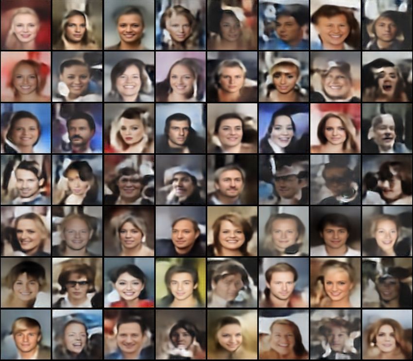
Published as a conference paper at ICLR 2021

While recent work has shown that using memory augmented neural networks can drastically improve
the performance of generative models (Wu et al., 2018a;b), language models (Weston et al., 2015),
meta-learning (Santoro et al., 2016), long-term planning (Graves et al., 2014; 2016) and sample
efficiency in reinforcement learning (Zhu et al., 2019), no model has been proposed to exploit
the inherent multi-dimensionality of biological memory Reimann et al. (2017). Inspired by the
traditional (computer-science) memory model of heap allocation (Figure 1-Left), we propose a
novel differentiable memory allocation scheme called Kanerva ++ (K++), that learns to compress
an episode of samples, referred to by the set of pointers {p1, ..., p4} in Figure 1, into a latent
multi-dimensional memory (Figure 1-Right). The K++ model infers a key distribution as a proxy
to the pointers (Marlow et al., 2008) and is able to embed similar samples to an overlapping latent
representation space, thus enabling it to be more efficient on compressing input distributions. In
this work, we focus on applying this novel memory allocation scheme to latent variable generative
models, where we improve the memory model in the Kanerva Machine (Wu et al., 2018a;b).

2   R ELATED W ORK
Variational Autoencoders: Variational autoencoders (VAEs) (Kingma & Welling, 2014) are a
fundamental part of the modern machine learning toolbox and have wide ranging applications
from generative modeling (Kingma & Welling, 2014; Kingma et al., 2016; Burda et al., 2016),
learning graphs (Kipf & Welling, 2016), medical applications (Sedai et al., 2017; Zhao et al., 2019)
and video analysis (Fan et al., 2020). As a latent variable model, VAEs infer an approximate
posterior over a latent representation Z and can be used in downstream tasks such as control in
reinforcement learning (Nair et al., 2018; Pritzel et al., 2017). VAEs maximize an evidence lower
bound (ELBO), L(X, Z), of the log-marginal likelihood, ln p(X) > L(X, Z) = ln pθ (X|Z) −
DKL (qφ (Z|X)||pθ (Z)). The produced variational approximation, qφ (Z|X), is typically called the
encoder, while pθ (X|Z) comes from the decoder. Methods that aim to improve these latent variable
generative models typically fall into two different paradigms: learning more informative priors or
leveraging novel decoders. While improved decoder models such as PixelVAE (Gulrajani et al.,
2017) and PixelVAE++ (Sadeghi et al., 2019) drastically improve the performance of pθ (X|Z),
they suffer from a phenomenon called posterior collapse (Lucas et al., 2019), where the decoder can
become almost independent of the posterior sample, but still retains the ability to reconstruct the
original sample by relying on its auto-regressive property (Goyal et al., 2017a).
In contrast, VampPrior (Tomczak & Welling, 2018), Associative Compression Networks (ACN)
(Graves et al., 2018), VAE-nCRP (Goyal et al., 2017b) and VLAE (Chen et al., 2017) tighten
the variational bound by learning more informed priors. VLAE for example, uses a powerful
auto-regressive prior; VAE-nCRP learns a non-parametric Chinese restaurant process prior and
VampPrior learns a Gaussian mixture prior representing prototypical virtual samples. On the other
hand, ACN takes a two-stage approach: by clustering real samples in the space of the posterior; and
by using these related samples as inputs to a learned prior, ACN provides an information theoretic
alternative to improved code transmission. Our work falls into this latter paradigm: we parameterize
a learned prior by reading from a common memory, built through a transformation of an episode of
input samples.
Memory Models: Inspired by the associative nature of biological memory, the Hopfield network
(Hopfield, 1982) introduced the notion of content-addressable memory, defined by a set of binary
neurons coupled with a Hamiltonian and a dynamical update rule. Iterating the update rule
minimizes the Hamiltonian, resulting in patterns being stored at different configurations (Hopfield,
1982; Krotov & Hopfield, 2016). Writing in a Hopfield network, thus corresponds to finding weight
configurations such that stored patterns become attractors via Hebbian rules (Hebb, 1949). This
concept of memory was extended to a distributed, continuous setting in Kanerva (1988) and to
a complex valued, holographic convolutional binding mechanism by Plate (1995). The central
difference between associative memory models Hopfield (1982); Kanerva (1988) and holographic
memory Plate (1995) is that the latter decouples the size of the memory from the input word size.
Most recent work with memory augmented neural networks treat memory in a slot-based manner
(closer to the associative memory paradigm), where each column of a memory matrix, M , represents
a single slot. Reading memory traces, z, entails using a vector of addressing weights, r, to attend
to the appropriate column of M , z = rT M . This paradigm of memory includes models such as
the Neural Turing Machine (NTM) (Graves et al., 2014), Differentiable Neural Computer (DNC)

                                                 2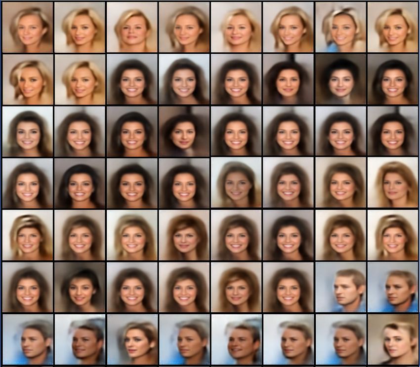
Published as a conference paper at ICLR 2021

(Graves et al., 2016) 1 , Memory Networks (Weston et al., 2015), Generative Temporal Models with
Memory (GTMM) Fraccaro et al. (2018), Variational Memory Encoder-Decoder (VMED) Le et al.
(2018), and Variational Memory Addressing (VMA) (Bornschein et al., 2017). VMA differs from
GTMM, VMED, DNC, NTM and Memory Networks by taking a stochastic approach to discrete
key-addressing, instead of the deterministic approach of the latter models.
Recently, the Kanerva Machine (KM) (Wu et al., 2018a) and its extension, the Dynamic Kanerva
Machine (DKM) (Wu et al., 2018b), interpreted memory writes and reads as inference in a generative
model, wherein memory is now treated as a distribution, p(M ). Under this framework, memory
reads and writes are recast as sampling or updating the memory posterior. The DKM model differs
from the KM model by introducing a dynamical addressing rule that could be used throughout
training. While providing an intuitive and theoretically sound bound on the data likelihood, the
DKM model requires an inner optimization loop which entails solving an ordinary least squares
(OLS) problem. Typical OLS solutions require a matrix inversion (O(n3 )), preventing the model
from scaling to large memory sizes. More recent work has focused on employing a product of
smaller Kanerva memories (Marblestone et al., 2020) in an effort to minimize the computational
cost of the matrix inversion. In contrast, we propose a simplified view of memory creation by
treating memory writes as a deterministic process in a fully feed-forward setting. Crucially, we
also modify the read operand such that it uses localized sub-regions of the memory, providing an
extra dimension of operation in comparison with the KM and DKM models. While the removal of
memory stochasticity might be interpreted as reducing the representation power of the model, we
empirically demonstrate through our experiments that our model performs better, trains quicker and
is simpler to optimize. The choice of a deterministic memory is further reinforced by research in
psychology, where human visual memory has been shown to change deterministically Gold et al.
(2005); Spencer & Hund (2002); Hollingworth et al. (2013).
3 M ODEL
To better understand the K++ model, we examine each of the individual components to understand
their role within the complete generative model. We begin by first deriving a conditional variational
lower bound (Section 3.1), describing the optimization objective and probabilistic assumptions. We
then describe the write operand (Section 3.3), the generative process (Section 3.4) and finally the
read and iterative read operands (Section 3.5).
3.1 P RELIMINARIES
K++ operates over an exchangeable episode (Aldous, 1985) of samples, X = {xt }Tt=1 ∈ D, drawn
from a dataset D, as in the Kanerva Machine. Therefore, the ordering of the samples within the
episode does not matter. This enables factoring the conditional, p(X|M ), over each of the individual
           QT
samples: t=1 p(xt |M ), given the memory, M ∼ p(M ), M ∈ RĈ×Ŵ ×Ĥ . Our objective in this
work is to maximize the expected conditional log-likelihood as in (Bornschein et al., 2017; Wu et al.,
2018a):
                                              Z Z                  XT
          J = Ep(X), p(M |X) ln pθ (X|M ) =          p(X)p(M |X)       ln pθ (xt |M )dXdM         (1)
                                                                        t=1

As alluded to in Barber & Agakov (2004) and Wu et al. (2018a), this objective can be interpreted as
maximizing the mutual information, I(X; M ), between the memory, M , and the episode, X, since
I(X; M ) = H(X) + J = H(X) − H(X; M ) and given that the entropy of the data, H(X), is
constant. In order to actualize Equation 1 we rely on a variational bound which we derive in the
following section.
3.2 VARIATIONAL L OWER B OUND
To efficiently read from the memory, M , we introduce a set of latent variables corresponding to
the K addressing read heads, Y = {Yt = {ytk }K        T            3
                                                 k=1 }t=1 , ytk ∈ R , and a set of latent variables
corresponding to the readout from the memory, Z = {zt }t=1 , zt ∈ RL . Given these latent variables,
                                                        T

we can decompose the conditional, ln p(X|M ), using the product rule and introduce variational
approximations qφ (Z|X) 2 and qφ (Y |X) via a multipy-by-one trick:

   1
     While DNC is slot based, it should be noted that DNC reads rows rather than columns.
   2
     We use qφ (Z|X) as our variational approximation instead of qφ (Z|X, Y, M ) in DKM as it presents a more
stable objective. We discuss this in more detail in Section 3.5.

                                                     3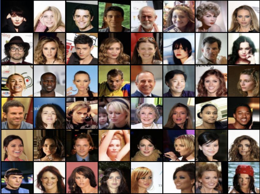
Published as a conference paper at ICLR 2021

                      p(X, Z, Y |M )         p(X|Z, M, Y ) p(Z|M, Y ) p(Y |M )
  ln p(X|M ) = ln                       = ln
                      p(Z, Y |X, M )              p(Z|M, Y, X) p(Y |M, X)

                                            p(X|Z, M, Y ) p(Z|M, Y ) p(Y ) qφ (Z|X) qφ (Y |X)
                  ≈ Eqφ (Z|X),qφ (Y |X) ln                                                      (2)
                                              p(Z|M, Y, X) p(Y |M, X) qφ (Z|X) qφ (Y |X)
                  = LT + Eqφ (Y |X) qφ (M |X,Y ) DKL (qφ (Z|X)||p(Z|M, Y, X))                   (3)
                           |                        {z                       }
                                                           ≥0
                         + DKL (qφ (Y |X)||p(Y |M, X))
                           |            {z           }
                                           ≥0
Equation 2 assumes that Y is independent from M : p(Y |M ) = p(Y ). This decomposition results in
Equation 3, which includes two KL-divergences against true (unknown) posteriors, p(Z|M, Y, X)
and p(Y |M, X). We can then train the model by maximizing the evidence lower bound (ELBO),
LT , to the true conditional, ln p(X|M ) > LT :
                            LT = Eqφ (Z|X), qφ (Y |X) ln pθ (X|Z, M, Y )
                                 |                  {z                 }
                                                        Decoder
                                   − Eqφ (Y |X) DKL [qφ (Z|X)||pθ (Z|M, Y )]                        (4)
                                     |                   {z                }
                                     Amortized latent variable posterior vs. memory readout prior

                                   − DKL [qφ (Y |X)||p(Y )]
                                     |         {z         }
                                     Amortized key posterior vs. key prior
The bound in Equation 4 is tight if qφ (Z|X) = p(Z|M, Y, X) and qφ (Y |X) = p(Y |M, X),
however, it involves inferring the entire memory M ∼ qφ (M |X, Y ). This prevents us from
decoupling the size of the memory from inference and scales the computation complexity based
on the size of the memory. To alleviate this constraint, we assume a purely deterministic memory,
M ∼ δ[fmem (fenc (X))], built by transforming the input episode, X, via a deterministic encoder
and memory transformation model, fmem ◦ fenc . We also assume that the regions of memory which
are useful in reconstructing a sample, xt , can be summarized by a set of K localized contiguous
memory sub-blocks as described in Equation 5 below. The intuition here is that similar samples,
xt ≈ xr , might occupy a disjoint part of the representation space and the decoder, pθ (X|·), would
need to read multiple regions to properly handle sample reconstruction. For example, the digit “3”
might share part of the
                      representation space with a “2” and another part
                                                                     with a “5”.
                 M̂ ∼ δ {mk = fST (M = fmem (fenc (X)), ytk )}K
                                                              k=1 ≈ qφ (M |X, Y )                   (5)
M̂ in equation 5 represents a set of K dirac-delta memory sub-regions, determined by the addressing
key, ytk , and a spatial transformer (ST ) network Jaderberg et al. (2015), fST 3 . Our final
optimization objective, LT , is attained by approximating M ∼ qφ (M |X, Y ) from Equation 4 with
M̂ (Equation 5) and is summarized by the graphical model in 2 below.

Figure 2: (a): Generative model (§3.4). (b): Read inference model (§3.5). (c): Iterative read
inference model (§3.5). (d): Write inference model (§3.3). Dashed lines represent approximate
inference, while solid lines represent computing of a conditional distribution. Double sided arrow
in (c) represents the KL divergence between qφ (Z|X) and pθ (Z|M, Y ) from Equation 4. Squares
represent deterministic nodes. Standard plate notation is used to depict a repetitive operation.
   3
       We provide a brief review of spatial transformers in Appendix A

                                                            4
Published as a conference paper at ICLR 2021

3.3   W RITE M ODEL

                                                                         sample episode:
                                                                           Xt = {x1 , ..., xT } ∼ D;
                                                                         compute embedding:
                                                                           E = fθenc (Xt ) ;
                                                                         infer keys: Yt ∼
                                                                           N (µθkey (E), σθ2key (E)) ;
                                                                         write memory:
                                                                           M ∼ δ(fθmem (E))

                        Figure 3: Left: Write model. Right: Write operation.

Writing to memory in the K++ model (Figure 3) entails encoding the input episode, Xt = {xt }Tt=1 ,
through the encoder, E = fθenc (Xt ), pooling the representation over the episode and encoding
the pooled representation with the memory writer, M = fθmem (E). In this work, we employ a
Temporal Shift Module (TSM) (Lin et al., 2019), applied on a ResNet18 (He et al., 2016). TSM
works by shifting feature maps of a two-dimensional vision model in the temporal dimension in
order to build richer representations of contextual features. In the case of K++, this allows the
encoder to build a better representation of the memory by leveraging intermediary episode specific
features. Using a TSM encoder over a standard convolutional stack improves the performance of
both K++ and DKM, where the latter observes an improvement of 6.32 nats/image over the reported
test conditional variational lower bound of 77.2 nats/image (Wu et al., 2018b) for the binarized
Omniglot dataset. As far as we are aware, the application of a TSM encoder to memory models has
not been explored and is a contribution of this work.
The memory writer model, fθmem , in Figure 3, allows K++ to non-linearly transform the pooled
embedding to better summarize the episode. In addition to inferring the deterministic memory, M ,
we also project the non-pooled embedding, E, through a key model, fθkey :

                 {Yt }Tt=1 = µθkey (E) + σθ2key (E)     , ytk ∈ R3 ,  ∼ N (0, 1).                        (6)

The reparameterized keys will be used to read sample specific memory traces, M̂ , from the full
memory, M . The memory traces, M̂ , are used in training through the learned prior, pθ (Z|M̂ , Y ) =
N (µz , σz2 ), from Equation 4 via the KL divergence, Eqφ (Y |X) DKL [qφ (Z|X)||Pθ (Z|M̂ , Y )]. This
KL divergence constrains the optimization objective to keep the representation of the amortized
approximate posterior, qφ (Z|X), (probabilistically) close to the memory readout representation of
the learned prior, pθ (Z|M̂ , Y ). In the generative setting, this constraint enables memory traces to be
routed from the learned prior, pθ (Z|M̂ , Y ), to the decoder, pθ (X|·), in a similar manner to standard
VAEs. We detail this process in the following section.
3.4   S AMPLE G ENERATION

                                                                           given memory: M ;
                                                                           sample keys: Yt ∼ P (Yt );
                                                                           extract regions: M̂ =
                                                                             {fθST (M, ytk )}K k=1 ;
                                                                           infer latent: Zt ∼
                                                                             N (µθZ (M̂ ), σθ2Z (M̂ )) ;
                                                                           decode: X̂t ∼
                                                                             N (µθdec (µZt ), σ 2 )

                   Figure 4: Left: Generative model. Right: Generative operation.

                                                   5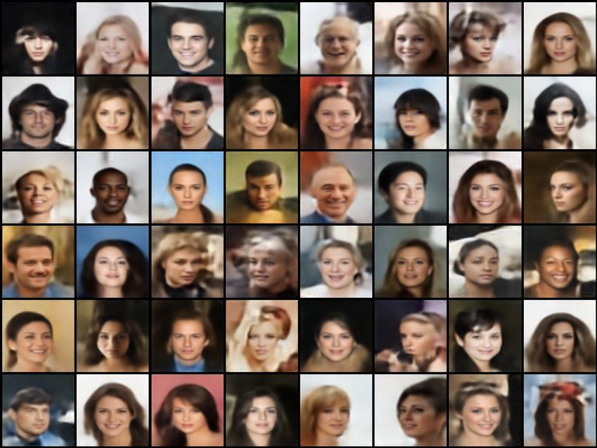
Published as a conference paper at ICLR 2021

The Kanerva++ model, like the original KM and DKM models, enables sample generation given
an existing memory or set of memories. K samples from the prior key distribution, {yk }K       k=1 ∼
p(Y ) = N (0, 1), yk ∈ R3 , are used to parameterize the spatial transformer, fST , which indexes the
deterministic memory, M . The result of this differentiable indexing is a set of memory sub-regions,
M̂ , which are used in the decoder, pθ (X|·), to generate synthetic samples. Reading samples in
this manner forces the encoder to utilize memory sub-regions that are useful for reconstruction, as
non-read memory regions receive zero gradients during backpropagation. This insight allows us to
use the simple feed-foward write process described in Section 3.3, while still retaining the ability to
produce locally contiguous block allocated memory.

3.5   R EAD / I TERATIVE R EAD M ODEL

                                                                            given embedding: E ;
                                                                            if training then
                                                                                 infer latent: Zt ∼
                                                                                   N (µθz (E), σθ2z (E))
                                                                                 infer prior: Zt ∼
                                                                                   N (µθz (M̂ ), σθ2z (M̂ ))
                                                                            else
                                                                                 infer latent: Zt ∼
                                                                                   N (µθz (M̂ ), σθ2z (M̂ ))
                                                                            end
                                                                            decode: X̂t ∼
                                                                              N (µθdec (µZt ), σ 2 )
Figure 5: Left: Read model: bottom branch from embedding used during iterative reading and prior
evaluation. Stable top branch used to infer qφ (Z|X) during training. Right: Read operation.

K++ involves two forms of reading (Figure 5): iterative reading and a simpler and more stable
read model used for training. During training we actualize qφ (Z|X) from Equation 4 using an
amortized isotropic-gaussian posterior that directly transforms the embedding of the episode, E,
using a learned neural network (Figure 2-b). As mentioned in Section 3.5, the readout, Z, of
the memory traces, M̂ , are encouraged to learn a meaningful structured representation through
the memory read-out KL divergence, Eqφ (Y |X) DKL [qφ (Z|X)||Pθ (Z|M̂ , Y )], which attempts to
minimize the (probabilistic) distance between qφ (Z|X) and Pθ (Z|M̂ , Y ).
Kanerva memory models also possess the ability to gradually improve a sample through interative
inference (Figure 2-c), whereby noisy samples can be improved by leveraging contextual
information stored in memory. This can be interpreted as approximating the posterior, q(Z|X, M ),
by marginalizing the approximate key distribution:
                              Z
                q(Z|X, M̂ ) = qφ (Y |X)pθ (Z|Y, M̂ )δY ≈ pθ (Z|Y = Y ∗ , M̂ ),                (7)

where Y ∗ ∼ qφ (Y |X = X̂) in Equation 7 uses a single sample Monte Carlo estimate, evaluated by
re-infering the previous reconstruction, X̂ ∼ pθ (X|·), through the approximate key posterior. Each
subsequent memory readout, Z, improves upon its previous representation by absorbing additional
information from the memory.

4     E XPERIMENTS
We contrast K++ against state-of-the-art memory conditional vision models and present empirical
results in Table 1. Binarized datasets assume Bernoulli output distributions, while continuous values
are modeled by a discretized mixture of logistics Salimans et al. (2017). As is standard in literature
Burda et al. (2016); Sadeghi et al. (2019); Ma et al. (2018); Chen et al. (2017), we provide results
for binarized MNIST and binarized Omniglot in nats/image and rescale the corresponding results to
bits/dim for all other datasets. We describe the model architecture, the optimization procedure and
the memory creation protocol in Appendix E and E.1. Finally, extra Celeb-A generations and test
image reconstructions for all experiments are provided in Appendix B and Appendix D respectively.

                                                  6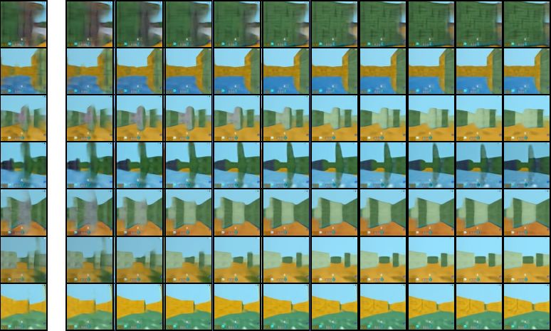
Published as a conference paper at ICLR 2021

                                        Binarized        Binarized        Fashion      CIFAR10          DMLab
              Method                     MNIST           Omniglot         MNIST                         Mazes
                                      (nats / image)   (nats / image)   (bits / dim)   (bits / dim)   (bits / dim)
 VAE Kingma & Welling (2014)          87.86            104.75           5.84           6.3            -
 IWAE Burda et al. (2016)             85.32            103.38           -              -              -
 Improved decoders
 PixelVAE++ Sadeghi et al. (2019)     78.00            -                -              2.90           -
 MAE Ma et al. (2018)                 77.98            89.09            -              2.95           -
 DRAW Gregor et al. (2015)            87.4             96.5             -              3.58           -
 MatNet Bachman (2016)                78.5             89.5             -              3.24           -
 Richer priors
 Ordered ACN Graves et al. (2018)     ≤73.9            -                -              ≤3.07          -
 VLAE Chen et al. (2017)              78.53            102.11           -              2.95           -
 VampPrior Tomczak & Welling (2018)   78.45            89.76            -              -              -
 Memory conditioned models
 VMA Bornschein et al. (2017)         -                103.6            -              -              -
 KM Wu et al. (2018a)                 -                ≤68.3            -              ≤4.37+         -
 DNC Graves et al. (2016)             -                ≤100             -              -              -
 DKM Wu et al. (2018b)                ≤75.3∗           ≤77.2            -              ≤4.79∗         ≤2.75†
 DKM w/TSM (our impl)                 ≤51.84           ≤70.88           ≤4.15          ≤4.31          ≤2.92†
 Kanerva++ (ours)                     ≤41.58           ≤66.24           ≤3.40          ≤3.28          ≤2.88†
Table 1: Negative test likelihood and conditional test likelihood values (lower is better). ∗ was
graciously provided by original authors. + estimated from Wu et al. (2018a) Appendix Figure 12. †
variadic performance due to online generation of DMLab samples.
K++ presents state-of-the-art results for memory conditioned binarized MNIST and binarized
Omniglot, and presents competitive performance for Fashion MNIST, CIFAR10 and DMLab mazes.
The performance gap on the continuous valued datasets can be explained by our use of a simple
convolutional decoder, rather than the autoregressive decoders used in models such as PixelVAE
Sadeghi et al. (2019). We leave the exploration of more powerful decoder models to future work
and note that our model can be integrated with autoregressive decoders.
4.1   I TERATIVE INFERENCE

Figure 6: Left: First column to left visualizes first random key generation. Following columns
created by inferring previous sample through K++. Right: denoising of salt & pepper (top), speckle
(middle) and Poisson noise (bottom).
One of the benefits of K++ is that it uses the memory to learn a more informed prior by condensing
the information from an episode of samples. One might suspect that based on the dimensionality of
the memory and the size of the read traces, the memory might only learn prototypical patterns, rather
than a full amalgamation of the input episode. This presents a problem for generation, as described
in Section 3.4 , and can be observed in the first column of Figure 6-Left where the first generation
from a random key appears blurry. To overcome this limitation, we rely on the iterative inference
of Kanerva memory models (Wu et al., 2018a;b). By holding the memory, M , fixed and repeatedly
inferring the latents, we are able to clean-up the pattern by leveraging the contextual information
contained within the memory (§ 3.5). This is visualized in the proceeding columns of Figure 6-Left,
where we observe a slow but clear improvement in generation quality. This property of iterative
inference is one of the central benefits of using a memory model over a tradition solution like a
VAE. We also present results of iterative inference on more classical image noise distributions such
as salt-and-pepper, speckle and Poisson noise in Figure 6-Right. For each original noisy pattern (top
rows) we provide the resultant final reconstruction after ten steps of clean-up. The proposed K++ is
robust to input noise and is able to clean-up most of the patterns in a semantically meaningful way.

                                                       7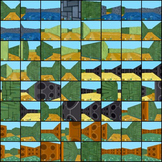
Published as a conference paper at ICLR 2021

4.1.1     I MAGE G ENERATIONS

      Figure 7: Key perturbed generations. Left: DMLab mazes. Center: Omniglot. Right: Celeb-A 64x64.

      Figure 8: Random key generations. Left: DMLab mazes. Center: Omniglot. Right: Celeb-A 64x64.
Typical VAEs use high dimensional isotropic Gaussian latent variables (≥ R16 ) Burda et al. (2016);
Kingma & Welling (2014). A well known property of high dimensional Gaussian distributions is
that most of their mass is concentrated on the surface area of a high dimensional ball. Perturbations
to a sample in an area of valid density can easily move it to an invalid density region (Arvanitidis
et al., 2018; White, 2016), causing blurry or irregular generations. In the case of K++, since the key
distribution, yt ∼ p(Y ), yt ∈ R3 , is within a low dimensional space, local perturbations, yt + ,  ∼
N (0, 0.1), are likely in regions with high probability density. We visualize this form of generation
in Figure 7 for DMLab Mazes, Omniglot and Celeb-A 64x64, as well as the more traditional random
key generations, yt ∼ p(Y ), in Figure 8.
Interestingly, local key perturbations of a trained DMLab Maze K++ model induces resultant
generations that provide a natural traversal of the maze as observed by scanning Figure 7-Left,
row by row, from left to right. In contrast, the random generations of the same task (Figure 8-Left)
present a more discontinuous set of generations. We see a similar effect for the Omniglot and
Celeb-A datasets, but observe that the locality is instead tied to character or facial structure as
shown in Figure 7-Center and Figure 7-Right. Finally, in contrast to VAE generations, K++ is able
to generate sharper images of ImageNet32x32 as shown in Appendix C. Future work will investigate
this form of locally perturbed generation through an MCMC lens.

4.2     A BLATION : I S B LOCK A LLOCATED S PATIAL M EMORY U SEFUL ?

Figure 9: Left: Simplified write model directly produces readout prior from Equation 4 by projecting
embedding E via a learned network. Right: Test negative variational lower bound (mean ±1std).

                                                    8
Published as a conference paper at ICLR 2021

While Figure 7 demonstrates the advantage of having a low dimensional sampling distribution and
Figure 6 demonstrates the benefit of iterative inference, it is unclear whether the performance benefit
in Table 1 is achieved from the episodic training, model structure, optimization procedure or memory
allocation scheme. To isolate the cause of the performance benefit, we simplify the write architecture
from Section 3.3 as shown in Figure 9-Left. In this scenario, we produce the learned memory
readout, Z, via an equivalently sized dense model that projects the embedding, E, while keeping all
other aspects the same. We train both models five times with the exact same TSM-ResNet18 encoder,
decoder, optimizer and learning rate scheduler. As shown in Figure 9-Right, the test conditional
variational lower bound of the K++ model is 20.6 nats/image better than the baseline model for the
evaluated binarized Omniglot dataset. This confirms that the spatial, block allocated latent memory
model proposed in this work is useful when working with image distributions. Future work will
explore this dimension for other modalities such as audio and text.

4.3   A BLATION : EPISODE LENGTH (T) AND MEMORY READ STEPS (K).

Figure 10: Binarized MNIST. Left: Episode length (T) ablation showing negative test conditional
variational lower bound (mean±std). Right: Memory read steps (K) ablation showing test KL
divergence.
To further explore K++, we evaluate the sensitivity of the model to varying episode lengths (T) in
Figure 10-left and memory read steps (K) in Figure 10-right using the binarized MNIST dataset.
We train K++ five times (each) for episode lengths ranging from 5 to 64 and observe that the
model performs within margin of error for increasing episode lengths, producing negative test
conditional variational bounds within a 1-std of ±0.625 nats/image. This suggests that for the
specific dimensionality of memory (R64×64 ) used in this experiment, K++ was able to successfully
capture the semantics of the binarized MNIST distribution. We suspect that for larger datasets this
relationship might not necessary hold and that the dimensionality of the memory should scale with
the size of the dataset, but leave the prospect of such capacity analysis for future research.
While ablating the number of memory reads (K) in Figure 10-right, we observe that the total test
KL-divergence varies by 1-std of ±0.041 nats/image for a range of memory reads from 1 to 64. A
lower KL divergence implies that the model is able to better fit the approximate posteriors qφ (Z|X)
and qφ (Y |X) to their correspondings priors in Equation 4. It should however be noted that a
lower KL-divergence does not necessary imply a better generative model Theis et al. (2016). While
qualitatively inspecting the generated samples, we observed that K++ generated more semantically
sound generations at lower memory read steps. We suspect that the difficulty of generating realistic
samples increases with the number of disjoint reads and found that K = 2 produces high quality
results. We use this value for all experiments in this work.

5     C ONCLUSION
In this work, we propose a novel block allocated memory in a generative model framework and
demonstrate its state-of-the-art performance on several memory conditional image generation tasks.
We also show that stochasticity in low-dimensional spaces produces higher quality samples in
comparison to high-dimensional latents typically used in VAEs. Furthermore, perturbations to
the low-dimensional key generate samples with high variations. Nonetheless, there are still many
unanswered questions: would a hard attention based solution to differentiable indexing prove to be
better than a spatial transformer? What is the optimal upper bound of window read regions based
on the input distribution? Future work will hopefully be able to address these lingering issues and
further improve generative memory models.

                                                  9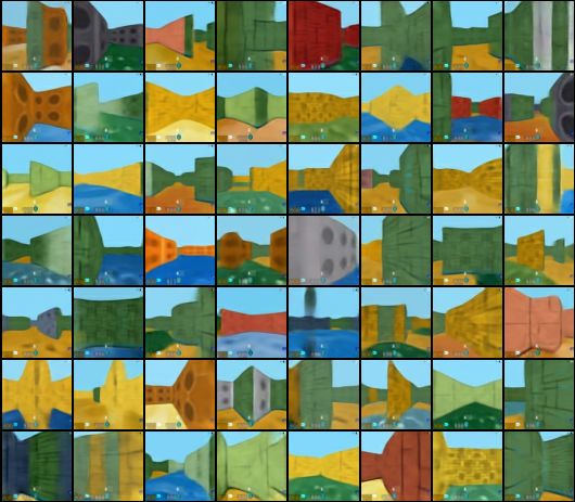
Published as a conference paper at ICLR 2021

R EFERENCES
David J Aldous. Exchangeability and related topics. In École d’Été de Probabilités de Saint-Flour
  XIII—1983, pp. 1–198. Springer, 1985.
Georgios Arvanitidis, Lars Kai Hansen, and Søren Hauberg. Latent space oddity: On the curvature
  of deep generative models. In 6th International Conference on Learning Representations, ICLR
  2018, 2018.
Philip Bachman.      An architecture for deep, hierarchical generative models.     In
  Daniel D. Lee, Masashi Sugiyama, Ulrike von Luxburg, Isabelle Guyon, and Roman
  Garnett (eds.), Advances in Neural Information Processing Systems 29:        Annual
  Conference on Neural Information Processing Systems 2016, December 5-10, 2016,
  Barcelona, Spain, pp. 4826–4834, 2016. URL http://papers.nips.cc/paper/
  6141-an-architecture-for-deep-hierarchical-generative-models.
David Barber and Felix V Agakov. Information maximization in noisy channels: A variational
  approach. In Advances in Neural Information Processing Systems, pp. 201–208, 2004.
Jörg Bornschein, Andriy Mnih, Daniel Zoran, and Danilo Jimenez Rezende. Variational memory
   addressing in generative models. In Advances in Neural Information Processing Systems, pp.
   3920–3929, 2017.
Yuri Burda, Roger B. Grosse, and Ruslan Salakhutdinov. Importance weighted autoencoders.
  In Yoshua Bengio and Yann LeCun (eds.), 4th International Conference on Learning
  Representations, ICLR 2016, San Juan, Puerto Rico, May 2-4, 2016, Conference Track
  Proceedings, 2016. URL http://arxiv.org/abs/1509.00519.
Xi Chen, Diederik P Kingma, Tim Salimans, Yan Duan, Prafulla Dhariwal, John Schulman, Ilya
  Sutskever, and Pieter Abbeel. Variational lossy autoencoder. ICLR, 2017.
Yaxiang Fan, Gongjian Wen, Deren Li, Shaohua Qiu, Martin D Levine, and Fei Xiao. Video anomaly
  detection and localization via gaussian mixture fully convolutional variational autoencoder.
  Computer Vision and Image Understanding, pp. 102920, 2020.
Marco Fraccaro, Danilo Jimenez Rezende, Yori Zwols, Alexander Pritzel, S. M. Ali Eslami,
 and Fabio Viola. Generative temporal models with spatial memory for partially observed
 environments. In Jennifer G. Dy and Andreas Krause (eds.), Proceedings of the 35th International
 Conference on Machine Learning, ICML 2018, Stockholmsmässan, Stockholm, Sweden, July
 10-15, 2018, volume 80 of Proceedings of Machine Learning Research, pp. 1544–1553. PMLR,
 2018. URL http://proceedings.mlr.press/v80/fraccaro18a.html.
Jason M Gold, Richard F Murray, Allison B Sekuler, Patrick J Bennett, and Robert Sekuler. Visual
  memory decay is deterministic. Psychological Science, 16(10):769–774, 2005.
Anirudh Goyal Alias Parth Goyal, Alessandro Sordoni, Marc-Alexandre Côté, Nan Rosemary Ke,
  and Yoshua Bengio. Z-forcing: Training stochastic recurrent networks. In Advances in neural
  information processing systems, pp. 6713–6723, 2017a.
Prasoon Goyal, Zhiting Hu, Xiaodan Liang, Chenyu Wang, and Eric P Xing. Nonparametric
  variational auto-encoders for hierarchical representation learning. In Proceedings of the IEEE
  International Conference on Computer Vision, pp. 5094–5102, 2017b.
Priya Goyal, Piotr Dollár, Ross B. Girshick, Pieter Noordhuis, Lukasz Wesolowski, Aapo Kyrola,
  Andrew Tulloch, Yangqing Jia, and Kaiming He. Accurate, large minibatch SGD: training
  imagenet in 1 hour. CoRR, abs/1706.02677, 2017c. URL http://arxiv.org/abs/1706.
  02677.
Alex Graves, Greg Wayne, and Ivo Danihelka.             Neural turing machines.      arXiv preprint
  arXiv:1410.5401, 2014.
Alex Graves, Greg Wayne, Malcolm Reynolds, Tim Harley, Ivo Danihelka, Agnieszka
  Grabska-Barwińska, Sergio Gómez Colmenarejo, Edward Grefenstette, Tiago Ramalho, John
  Agapiou, et al. Hybrid computing using a neural network with dynamic external memory. Nature,
  538(7626):471–476, 2016.

                                                 10
Published as a conference paper at ICLR 2021
Alex Graves, Jacob Menick, and Aaron van den Oord. Associative compression networks for
representation learning. arXiv preprint arXiv:1804.02476, 2018.
Karol Gregor, Ivo Danihelka, Alex Graves, Danilo Rezende, and Daan Wierstra. Draw: A recurrent
neural network for image generation. In International Conference on Machine Learning, pp.
1462–1471, 2015.
Ishaan Gulrajani, Kundan Kumar, Faruk Ahmed, Adrien Ali Taı̈ga, Francesco Visin, David Vázquez,
and Aaron C. Courville. Pixelvae: A latent variable model for natural images. In 5th
International Conference on Learning Representations, ICLR 2017, Toulon, France, April 24-26,
2017, Conference Track Proceedings. OpenReview.net, 2017. URL https://openreview.
net/forum?id=BJKYvt5lg.
Kaiming He, Xiangyu Zhang, Shaoqing Ren, and Jian Sun. Deep residual learning for image
recognition. In Proceedings of the IEEE Conference on Computer Vision and Pattern Recognition,
pp. 770–778, 2016.
Donald Olding Hebb. The organization of behavior: a neuropsychological theory. J. Wiley;
Chapman & Hall, 1949.
Andrew Hollingworth, Michi Matsukura, and Steven J Luck. Visual working memory modulates
rapid eye movements to simple onset targets. Psychological science, 24(5):790–796, 2013.
John J Hopfield. Neural networks and physical systems with emergent collective computational
abilities. Proceedings of the national academy of sciences, 79(8):2554–2558, 1982.
Sergey Ioffe and Christian Szegedy. Batch normalization: Accelerating deep network training by
reducing internal covariate shift. In Francis R. Bach and David M. Blei (eds.), Proceedings of the
32nd International Conference on Machine Learning, ICML 2015, Lille, France, 6-11 July 2015,
volume 37 of JMLR Workshop and Conference Proceedings, pp. 448–456. JMLR.org, 2015. URL
http://proceedings.mlr.press/v37/ioffe15.html.
Max Jaderberg, Karen Simonyan, Andrew Zisserman, et al. Spatial transformer networks. In
Advances in neural information processing systems, pp. 2017–2025, 2015.
Pentti Kanerva. Sparse distributed memory. MIT press, 1988.
Diederik P. Kingma and Jimmy Ba. Adam: A method for stochastic optimization. In Proceedings
of the 3rd International Conference on Learning Representations (ICLR), 2014.
Durk P. Kingma and Max Welling. Auto-encoding variational bayes. ICLR, 2014.
Durk P Kingma, Tim Salimans, Rafal Jozefowicz, Xi Chen, Ilya Sutskever, and Max Welling.
Improved variational inference with inverse autoregressive flow. In Advances in neural
information processing systems, pp. 4743–4751, 2016.
Thomas N. Kipf and Max Welling. Variational graph auto-encoders. CoRR, abs/1611.07308, 2016.
URL http://arxiv.org/abs/1611.07308.
Dmitry Krotov and John J Hopfield. Dense associative memory for pattern recognition. In Advances
in neural information processing systems, pp. 1172–1180, 2016.
Dharshan Kumaran, Demis Hassabis, and James L McClelland. What learning systems do intelligent
agents need? complementary learning systems theory updated. Trends in cognitive sciences, 20
(7):512–534, 2016.
Hung Le, Truyen Tran, Thin Nguyen, and Svetha Venkatesh. Variational memory encoder-decoder.
In Advances in Neural Information Processing Systems, pp. 1508–1518, 2018.
Ji Lin, Chuang Gan, and Song Han. Tsm: Temporal shift module for efficient video understanding.
In Proceedings of the IEEE International Conference on Computer Vision, pp. 7083–7093, 2019.
Hanxiao Liu, Andrew Brock, Karen Simonyan, and Quoc V. Le. Evolving normalization-activation
layers. CoRR, abs/2004.02967, 2020. URL https://arxiv.org/abs/2004.02967.
11Published as a conference paper at ICLR 2021
Ilya Loshchilov and Frank Hutter. SGDR: stochastic gradient descent with warm restarts. In 5th
International Conference on Learning Representations, ICLR 2017, Toulon, France, April 24-26,
2017, Conference Track Proceedings. OpenReview.net, 2017. URL https://openreview.
net/forum?id=Skq89Scxx.
James Lucas, George Tucker, Roger B. Grosse, and Mohammad Norouzi. Understanding
posterior collapse in generative latent variable models. In Deep Generative Models for Highly
Structured Data, ICLR 2019 Workshop, New Orleans, Louisiana, United States, May 6, 2019.
OpenReview.net, 2019. URL https://openreview.net/forum?id=r1xaVLUYuE.
Xuezhe Ma, Chunting Zhou, and Eduard Hovy. Mae: Mutual posterior-divergence regularization
for variational autoencoders. In International Conference on Learning Representations, 2018.
Adam Marblestone, Yan Wu, and Greg Wayne. Product kanerva machines: Factorized bayesian
memory. Bridging AI and Cognitive Science Workshop. ICLR, 2020.
Simon Marlow, Tim Harris, Roshan P James, and Simon Peyton Jones. Parallel generational-copying
garbage collection with a block-structured heap. In Proceedings of the 7th international
symposium on Memory management, pp. 11–20. ACM, 2008.
James L McClelland, Bruce L McNaughton, and Randall C O’Reilly. Why there are complementary
learning systems in the hippocampus and neocortex: insights from the successes and failures of
connectionist models of learning and memory. Psychological review, 102(3):419, 1995.
Takeru Miyato, Toshiki Kataoka, Masanori Koyama, and Yuichi Yoshida. Spectral normalization for
generative adversarial networks. In 6th International Conference on Learning Representations,
ICLR 2018, Vancouver, BC, Canada, April 30 - May 3, 2018, Conference Track Proceedings.
OpenReview.net, 2018. URL https://openreview.net/forum?id=B1QRgziT-.
Ashvin Nair, Vitchyr Pong, Murtaza Dalal, Shikhar Bahl, Steven Lin, and Sergey Levine.
Visual reinforcement learning with imagined goals. In Samy Bengio, Hanna M.
Wallach, Hugo Larochelle, Kristen Grauman, Nicolò Cesa-Bianchi, and Roman Garnett
(eds.), Advances in Neural Information Processing Systems 31: Annual Conference
on Neural Information Processing Systems 2018, NeurIPS 2018, 3-8 December 2018,
Montréal, Canada, pp. 9209–9220, 2018. URL http://papers.nips.cc/paper/
8132-visual-reinforcement-learning-with-imagined-goals.
Vinod Nair and Geoffrey E. Hinton. Rectified linear units improve restricted boltzmann machines.
In Johannes Fürnkranz and Thorsten Joachims (eds.), Proceedings of the 27th International
Conference on Machine Learning (ICML-10), June 21-24, 2010, Haifa, Israel, pp. 807–814.
Omnipress, 2010. URL https://icml.cc/Conferences/2010/papers/432.pdf.
Tony A Plate. Holographic reduced representations. IEEE Transactions on Neural networks, 6(3):
623–641, 1995.
Alexander Pritzel, Benigno Uria, Sriram Srinivasan, Adrià Puigdomènech Badia, Oriol Vinyals,
Demis Hassabis, Daan Wierstra, and Charles Blundell. Neural episodic control. In Doina
Precup and Yee Whye Teh (eds.), Proceedings of the 34th International Conference on Machine
Learning, ICML 2017, Sydney, NSW, Australia, 6-11 August 2017, volume 70 of Proceedings of
Machine Learning Research, pp. 2827–2836. PMLR, 2017. URL http://proceedings.
mlr.press/v70/pritzel17a.html.
Prajit Ramachandran, Barret Zoph, and Quoc V. Le. Searching for activation functions. In 6th
International Conference on Learning Representations, ICLR 2018, Vancouver, BC, Canada,
April 30 - May 3, 2018, Workshop Track Proceedings. OpenReview.net, 2018. URL https:
//openreview.net/forum?id=Hkuq2EkPf.
Michael W. Reimann, Max Nolte, Martina Scolamiero, Katharine Turner, Rodrigo Perin, Giuseppe
Chindemi, Paweł Dłotko, Ran Levi, Kathryn Hess, and Henry Markram. Cliques of neurons
bound into cavities provide a missing link between structure and function. Frontiers in
Computational Neuroscience, 11:48, 2017. ISSN 1662-5188. doi: 10.3389/fncom.2017.00048.
URL https://www.frontiersin.org/article/10.3389/fncom.2017.00048.
12Published as a conference paper at ICLR 2021
Hossein Sadeghi, Evgeny Andriyash, Walter Vinci, Lorenzo Buffoni, and Mohammad H. Amin.
Pixelvae++: Improved pixelvae with discrete prior. CoRR, abs/1908.09948, 2019. URL http:
//arxiv.org/abs/1908.09948.
Tim Salimans, Andrej Karpathy, Xi Chen, and Diederik P. Kingma. Pixelcnn++: Improving the
pixelcnn with discretized logistic mixture likelihood and other modifications. In 5th International
Conference on Learning Representations, ICLR 2017, Toulon, France, April 24-26, 2017,
Conference Track Proceedings. OpenReview.net, 2017. URL https://openreview.net/
forum?id=BJrFC6ceg.
Adam Santoro, Sergey Bartunov, Matthew Botvinick, Daan Wierstra, and Timothy P. Lillicrap.
Meta-learning with memory-augmented neural networks. In Maria-Florina Balcan and Kilian Q.
Weinberger (eds.), Proceedings of the 33nd International Conference on Machine Learning,
ICML 2016, New York City, NY, USA, June 19-24, 2016, volume 48 of JMLR Workshop and
Conference Proceedings, pp. 1842–1850. JMLR.org, 2016. URL http://proceedings.
mlr.press/v48/santoro16.html.
Suman Sedai, Dwarikanath Mahapatra, Sajini Hewavitharanage, Stefan Maetschke, and Rahil
Garnavi. Semi-supervised segmentation of optic cup in retinal fundus images using variational
autoencoder. In International Conference on Medical Image Computing and Computer-Assisted
Intervention, pp. 75–82. Springer, 2017.
Leslie N. Smith and Nicholay Topin. Super-convergence: Very fast training of residual networks
using large learning rates. CoRR, abs/1708.07120, 2017. URL http://arxiv.org/abs/
1708.07120.
John P Spencer and Alycia M Hund. Prototypes and particulars: Geometric and
experience-dependent spatial categories. Journal of Experimental Psychology: General, 131(1):
16, 2002.
Lucas Theis, Aäron van den Oord, and Matthias Bethge. A note on the evaluation of generative
models. In Yoshua Bengio and Yann LeCun (eds.), 4th International Conference on Learning
Representations, ICLR 2016, San Juan, Puerto Rico, May 2-4, 2016, Conference Track
Proceedings, 2016. URL http://arxiv.org/abs/1511.01844.
Jakub Tomczak and Max Welling. Vae with a vampprior. In International Conference on Artificial
Intelligence and Statistics, pp. 1214–1223, 2018.
Jason Weston, Sumit Chopra, and Antoine Bordes. Memory networks. In Yoshua Bengio and Yann
LeCun (eds.), 3rd International Conference on Learning Representations, ICLR 2015, San Diego,
CA, USA, May 7-9, 2015, Conference Track Proceedings, 2015. URL http://arxiv.org/
abs/1410.3916.
Tom White. Sampling generative networks. arXiv preprint arXiv:1609.04468, 2016.
Yan Wu, Greg Wayne, Alex Graves, and Timothy Lillicrap. The kanerva machine: A generative
distributed memory. ICLR, 2018a.
Yan Wu, Gregory Wayne, Karol Gregor, and Timothy Lillicrap. Learning attractor dynamics for
generative memory. In Advances in Neural Information Processing Systems, pp. 9379–9388,
2018b.
Yuxin Wu and Kaiming He. Group normalization. Int. J. Comput. Vis., 128(3):742–755,
2020. doi: 10.1007/s11263-019-01198-w. URL https://doi.org/10.1007/
s11263-019-01198-w.
Yang You, Igor Gitman, and Boris Ginsburg. Large batch training of convolutional networks. arXiv
preprint arXiv:1708.03888, 2017.
Qingyu Zhao, Nicolas Honnorat, Ehsan Adeli, Adolf Pfefferbaum, Edith V Sullivan, and Kilian M
Pohl. Variational autoencoder with truncated mixture of gaussians for functional connectivity
analysis. In International Conference on Information Processing in Medical Imaging, pp.
867–879. Springer, 2019.
13Published as a conference paper at ICLR 2021
Guangxiang Zhu, Zichuan Lin, Guangwen Yang, and Chongjie Zhang. Episodic reinforcement
learning with associative memory. In International Conference on Learning Representations,
2019.
14Published as a conference paper at ICLR 2021
A S PATIAL T RANSFORMER R EVIEW
Indexing a matrix, M [x : x + ∆x, y : y + ∆y], is typically a non-differentiable operation since
it involves hard cropping around an index. Spatial transformers (Jaderberg et al., 2015) provide a
solution to this problem by decoupling the problem into two differentiable operands:
1. Learn an affine transformation of coordinates.
2. Use a differntiable bilinear transformation.
s t
i i
The affine transformation of source coordinates, s , to target coordinates, t is defined as:
j j
t " is # " is #
i s 0 x y 0 y1
= js = 0 js (8)
jt 0 s y 0 y0 y2
1 1
s 0 x
Here, the affine transform, θ = has three learnable scalars: {s, x, y} which define a
0 s y
scaling and translation in i and j respectively. In the case of K++, these three scalars represent
the components of the key sample, {y0 , y1 , y2 } ∈ R3 as shown in Equation 8. After transforming
the co-ordinates (not to be confused with the actual data), spatial transformers learn a differentiable
bilinear transform which can be interpreted as learning a differentiable mask that is element-wise
multiplied by the original data, M :
J
X J
X
c
Mnr max(0, 1 − |itnr − r|) max(0, 1 − |jnr
t
− n|) (9)
n=−1 r=−1
0.5 0 0.3
Consider the following example where θ = ; this parameterization differntiably
0 0.5 0.5
extracts the region shown in Figure 11-Right from Figure 11-Left:
Figure 11: Spatial transformer example. Left: original image with region inlaid. Right: extracted grid.
The range of values for {s, x, y} is bound between [−1, 1], where the center of the image is [0, 0].
15Published as a conference paper at ICLR 2021
B C ELEB -A G ENERATIONS
Figure 12: Random key Celeb-A generations.
We present random key generations of Celeb-A 64x64, trained without center cropping in Figure
12.
C VAE VS . K++ I MAGE N ET 32 X 32 G ENERATIONS
Figure 13: ImageNet32x32 generations. Left: VAE; Right: K++.
Figure 13 shows the difference in generations of a standard VAE vs. K++. In contrast to the
standard VAE generation (Figure 13-Left), the K++ generations (Figure 13-Right) appear much
sharper, avoiding the blurry generations observed with standard VAEs.
16Published as a conference paper at ICLR 2021
D T EST I MAGE R ECONSTRUCTIONS
Figure 14: Binarized test reconstructions; top row are true samples. Left: Omniglot; Right: MNIST.
Figure 15: Test set reconstructions; top row are true samples. Left: ImageNet64x64. Right: DMLab Mazes.
17Published as a conference paper at ICLR 2021
Figure 16: Test set reconstructions; top row are true samples. Celeb-A 64x64.
E M ODEL A RCHITECTURE & T RAINING
Encoder: As mentioned in Section 3.3, we use a TSM-Resnet18 encoder with Batchnorm (Ioffe &
Szegedy, 2015) and ReLU activations (Nair & Hinton, 2010) for all tasks. We apply a fractional
shift of the feature maps by 0.125 as suggested by the authors.
18Published as a conference paper at ICLR 2021
Decoder: Our decoder is a simple conv-transpose network with EvoNormS0 (Liu et al., 2020)
inter-spliced between each layer. Evonorms0 is similar in stride to Groupnorm (Wu & He, 2020)
combined with the swish activation function (Ramachandran et al., 2018).
Optimizer & LR scheule: We use LARS (You et al., 2017) coupled with ADAM (Kingma & Ba,
2014) and a one-cycle (Smith & Topin, 2017) cosine learning rate schedule (Loshchilov & Hutter,
2017). A linear warm-up of 10 epochs (Goyal et al., 2017c) is also used for the schedule. A weight
decay of 1e − 3 is used on every parameter barring biases and the affine terms of batchnorm. Each
task is trained for 500 or 1000 epochs depending on the size of the dataset.
Dense models: All dense models such as our key network are simple three layer deep linear dense
models with a latent dimension of 512 coupled with spectral normalization (Miyato et al., 2018).
Memory writer: fθmem uses a deep linear conv-transpose decoder on the pooled embedding, E
with a base feature map projection size of 256 with a division by 2 per layer. We use a memory size
of R3×64×64 for all the experiments in this work.
Learned Prior: pθ (Z|M̂ , Y ) uses a convolutional encoder that stacks the K read traces,
{fST (M, ytk )}K
k=1 , along the channel dimension and projects it to the dimensionality of Z.
In practice, we observed that K++ is about 2x as fast (wall clock) compared to our re-implementation
of DKM. We mainly attribute this to not having to solve an inner OLS optimization loop for memory
inference.
E.1 M EMORY CREATION PROTOCOL
The memory creation protocol of K++ is similar in stride to that of the DKM model, given
the deterministic relaxations and addressing mechanism described in Sections 3.3 and 3.4. Each
memory, M ∼ δ[fmem (fenc (X))], is a function of an episode of samples, X = {xt }Tt=1 ∈ D. To
efficiently optimize the conditional lower bound in Equation 4, we parallelize the learning objective
using a set of minibatches, as is typical with the optimization of neural networks. As with the
DKM model, K++ computes the train and test conditional evidence lower bounds in Table 1, by first
inferring the memory, M ∼ δ[fmem (fenc (X))], from the input episode, followed by the read out
procedure as described in Section 3.5.
19You can also read