EcoDes-DK15: high-resolution ecological descriptors of vegetation and terrain derived from Denmark's national airborne laser scanning data set - ESSD
←
→
Page content transcription
If your browser does not render page correctly, please read the page content below

Earth Syst. Sci. Data, 14, 823–844, 2022
https://doi.org/10.5194/essd-14-823-2022
© Author(s) 2022. This work is distributed under
the Creative Commons Attribution 4.0 License.

        EcoDes-DK15: high-resolution ecological descriptors of
        vegetation and terrain derived from Denmark’s national
                   airborne laser scanning data set
                    Jakob J. Assmann1 , Jesper E. Moeslund2 , Urs A. Treier1,3 , and Signe Normand1,3
            1 Ecoinformatics and Biodiversity, Department of Biology, Aarhus University, Aarhus, 8000, Denmark
                     2 Biodiversity,Department of Ecoscience, Aarhus University, Rønde, 8410, Denmark
                      3 Center for Sustainable Landscapes Under Global Change, Department of Biology

                                          Aarhus University, Aarhus, 8000, Denmark
                                 Correspondence: Jakob J. Assmann (j.assmann@bio.au.dk)

                                      Received: 29 June 2021 – Discussion started: 14 July 2021
                         Revised: 5 January 2022 – Accepted: 8 January 2022 – Published: 23 February 2022

       Abstract. Biodiversity studies could strongly benefit from three-dimensional data on ecosystem structure de-
       rived from contemporary remote sensing technologies, such as light detection and ranging (lidar). Despite the
       increasing availability of such data at regional and national scales, the average ecologist has been limited in
       accessing them due to high requirements on computing power and remote sensing knowledge. We processed
       Denmark’s publicly available national airborne laser scanning (ALS) data set acquired in 2014/15, together with
       the accompanying elevation model, to compute 70 rasterised descriptors of interest for ecological studies. With
       a grain size of 10 m, these data products provide a snapshot of high-resolution measures including vegetation
       height, structure and density, as well as topographic descriptors including elevation, aspect, slope and wetness
       across more than 40 000 km2 covering almost all of Denmark’s terrestrial surface. The resulting data set is com-
       paratively small (∼ 94 GB, compressed 16.8 GB), and the raster data can be readily integrated into analytical
       workflows in software familiar to many ecologists (GIS software, R, Python). Source code and documentation
       for the processing workflow are openly available via a code repository, allowing for transfer to other ALS data
       sets, as well as modification or re-calculation of future instances of Denmark’s national ALS data set. We hope
       that our high-resolution ecological vegetation and terrain descriptors (EcoDes-DK15) will serve as an inspiration
       for the publication of further such data sets covering other countries and regions and that our rasterised data set
       will provide a baseline of the ecosystem structure for current and future studies of biodiversity, within Denmark
       and beyond. The full data set is available on Zenodo: https://doi.org/10.5281/zenodo.4756556 (Assmann et al.,
       2021); a 5 MB teaser subset is also available: https://doi.org/10.5281/zenodo.6035188 (Assmann et al., 2022a).

1   Introduction                                                   (such as monitoring and conservation) has remained com-
                                                                   paratively low (Bakx et al., 2019). The low uptake is likely
Over the last decades, airborne laser scanning (ALS) has be-       a consequence of the considerable challenges that remain in
come an established data source for providing fine-resolution      handling these very large data sets, which require special-
measures of terrain and vegetation structure in ecological re-     ist expertise and software, as well as substantial amounts of
search (Moeslund et al., 2019; Guo et al., 2017; Zellweger et      data storage and processing power (Meijer et al., 2020; Vo et
al., 2016). Despite its informative potential and the increas-     al., 2016; Pfeifer et al., 2014). Here, we address this issue for
ing number of openly available ALS data sets with regional         Denmark by providing a compact set of ecologically relevant
and national extents (Vo et al., 2016), the uptake of these        measures of terrain characteristics and vegetation structure
data sets for large-scale ecological research and applications

Published by Copernicus Publications.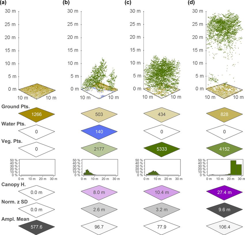
824                    J. J. Assmann et al.: EcoDes-DK15: high-resolution ecological descriptors of vegetation and terrain

derived as raster outputs from the country’s national ALS          that can be meaningfully derived from ALS data (Bakx et
data set with a grain size of 10 m × 10 m.                         al., 2019). This applies especially to the point cloud density,
   The typical output from an ALS survey is a so-called point      which needs to be high enough to meaningfully resolve the
cloud that describes the physical structure of the surveyed        structure of understorey layers in forests (Bakx et al., 2019)
area in three-dimensional space (Bakx et al., 2019; Vierling       or ecosystems with vegetation of low stature such as grass-
et al., 2008). In brief, short laser pulses are sent out from      lands or tundra (Boelman et al., 2016). Nonetheless, even
a light detection and ranging (lidar) sensor mounted on an         simpler ALS-derived descriptors of terrain and vegetation
aeroplane (or drone) and reflected by surfaces such as bare        structure can be of high value for ecological applications, as
ground, plants or buildings. The return timing of the reflected    fieldwork-derived alternatives are often too costly and diffi-
signal is measured and – with the help of information on the       cult to collect over large extents (Vierling et al., 2008).
sensor’s orientation and position – the precise location of the       ALS data have provided critical information for research
reflecting surface is determined in geographic space (Vier-        on biodiversity and habitat characteristics over recent years,
ling et al., 2008). If an object intercepting the light pulse is   and their importance in ecological research is likely to in-
smaller than the beam’s footprint (e.g. a leaf or a branch of      crease in the future. Numerous biodiversity studies have
a tree), some of the light may travel on and trigger a reflec-     successfully deployed ALS to study organisms like plants
tion from a second surface (e.g. understorey vegetation or         (Mao et al., 2018; Lopatin et al., 2016; Zellweger et al.,
the forest floor). A single light pulse might therefore gener-     2016; Ceballos et al., 2015; Moeslund et al., 2013; Leut-
ate two or even more returns, allowing – to some degree – for      ner et al., 2012), fungi (Peura et al., 2016; Thers et al.,
the penetration of forest canopies (Ackermann, 1999). Often,       2017), bryophytes, lichens (Moeslund et al., 2019), mammals
the raw signal is processed by the survey provider, and the        (Tweedy et al., 2019; Froidevaux et al., 2016) and birds (see
resulting data are delivered to the end user in the form of a      Bakx et al., 2019, for a comprehensive review) both in open
point cloud of discrete returns, in which each point is associ-    landscapes and in forests. These studies have all emphasised
ated with information on geographic location, return strength      the value of ALS for representing fine-scale (∼ 10 m resolu-
(amplitude), return number, acquisition timing, etc. (Vo et al.,   tion) terrain or vegetation structural variation important to lo-
2016). For ALS data sets with large extents – such as Den-         cal biodiversity patterns. Furthermore, Valbuena et al. (2020)
mark’s nationwide data set “DHM/Punktsky” – outputs from           recently considered ALS data to be one of the key resources
many survey flights are co-registered and merged, resulting        for deriving ecosystem morphological traits in the global as-
in very large point clouds with hundreds of billions of points     sessment of essential biodiversity variables (EBVs). Finding
and data volumes of multiple terabytes (Geodatastyrelsen,          ways of making regional and nationwide ALS data more ac-
2015). For further information on ALS data acquisition, we         cessible to the average ecologist is therefore not only a criti-
recommend Vo et al. (2016), Vierling et al. (2008), and Wag-       cal priority for accelerating research on regional biodiversity
ner et al. (2006).                                                 patterns and species–habitat relationships but also for the fa-
   Based on point position and neighbourhood context it is         cilitation of global assessments such as those carried out by
possible to separate ground and vegetation returns in ALS          IPBES (2019) and others alike.
point clouds, allowing for the calculation of descriptors of          To open up opportunities for researchers and practition-
terrain and vegetation structure. Filtering bare ground from       ers not familiar with ALS processing or without access to
the point cloud may be achieved with algorithms (Moudrý et         the required facilities, we present a new national ALS-based
al., 2020; Sithole and Vosselman, 2004), while more complex        data set for Denmark primarily aimed at ecological research
segmentation of the point clouds into object classes (such as      with possible uses in other disciplines. With a grain size of
vegetation, buildings, etc.) is done manually or with the help     10 m, these ecological descriptor (EcoDes) rasters provide a
of supervised machine learning (see Lin et al., 2020, for a        snapshot of high-resolution measures of vegetation height,
recent overview). Early applications for ALS were focussed         structure and density, as well as topographic descriptors
on generating simple digital elevation models (DEMs), city         including elevation, aspect, slope and wetness, for almost
and landscape planning, and forestry (Ackermann, 1999), but        all of Denmark’s terrestrial surface between spring 2014
over the last decades applications have expanded into other        and summer 2015 (DK15). In this publication, we (a) de-
fields, including, amongst others, the calculation of terrain      scribe the source data and outline the processing workflow
and vegetation measures for ecological research. Terrain-          (Sect. 2.1–2.3), (b) summarise the data set’s main charac-
derived measures of ecological interest include topographic        teristics (Sect. 3.1–3.2), (c) describe each descriptor in de-
slope, aspect (i.e. slope direction), solar irradiation, wet-      tail and highlight its use and limitations (Sect. 3.3–3.4), and
ness, etc. (e.g. Moeslund et al., 2019; Zellweger et al., 2016;    (d) provide guidance on data access and illustrate how the
Ceballos et al., 2015), and vegetation structural descriptors      data could be used in an example of ecological landscape
include vegetation density, canopy height diversity, canopy        classification (Sect. 4). We finish by (e) briefly discussing
roughness and many more (e.g. Bakx et al., 2019; Moeslund          the general limitations of the data set and processing work-
et al., 2019; Coops et al., 2016). It is important to note that    flow, as well as providing perspectives on how the presented
point cloud characteristics may limit the type of measures         data can be complemented with other data sources (Sect. 5).

Earth Syst. Sci. Data, 14, 823–844, 2022                                             https://doi.org/10.5194/essd-14-823-2022
J. J. Assmann et al.: EcoDes-DK15: high-resolution ecological descriptors of vegetation and terrain                              825

We hope that ease of access and thorough documentation of            system for Denmark (ETRS89/UTM zone 32N + DVR90
the EcoDes-DK15 data set will encourage uptake and facili-           height – EPSG:7416). The DHM/Terrain product is a ras-
tate the development of future versions of similar data sets in      terised digital model of the terrain height above sea level in
Denmark and beyond.                                                  0.4 m resolution. This product is provided in a 32 bit Geo-
                                                                     TIFF format, using the same 1 km × 1 km tiling convention
                                                                     and spatial reference system as the DHM/Point-cloud.
2     Source data and processing workflow overview
                                                                        The 1 km × 1 km tiling of the DHM/Terrain 2014/15 and
2.1    Denmark – geography and ecology
                                                                     DHM/Point-cloud 2014/15 data sets matches in extent and
                                                                     geolocation. However, a small number of tiles (n = 30) in
Located in northern Europe, Denmark (without Greenland               the DHM/Point-cloud data sets did not have corresponding
and the Faroe Islands) has an approximate land area of               tiles in the DHM/Terrain data sets; these were removed prior
43 000 km2 , comprising the large peninsula of Jutland and           to processing, resulting in the total of 49 673 tiles shown in
443 named islands. The relatively flat (highest point is 171 m       Table 1.
above sea level) landscape predominantly consists of arable
land and production forest with relatively small patches of          2.3   Processing
natural or semi-natural areas such as heathlands, grasslands,
fresh and salt meadows, bogs, dunes, lakes, streams, and de-         We processed the source data using OPALS 2.3.2.0 (Pfeifer
ciduous forests.                                                     et al., 2014), Python 2.7 (Van Rossum and Drake, 1995),
                                                                     pandas 0.24.2 (Reback et al., 2019), SAGA GIS 7.8.2 (Con-
2.2    ALS and elevation source data
                                                                     rad et al., 2015), and GDAL 2.2.4 (GDAL/OGR contribu-
                                                                     tors, 2018) from OSgeo4W64. Some re-processing was re-
The Danish elevation model (DHM) is an openly available              quired during the peer review process, for which we used
nationwide data set providing various products based on ALS          GDAL 3.3.3 from Osgeo4W64 (GDAL/OGR contributors,
data. Here, we used the DHM/Point-cloud (DHM/Punktsky),              2022). The large number of tiles and descriptors to be cal-
the classified georeferenced ALS point cloud product, and            culated required us to develop a robust processing pipeline,
the DHM/Terrain (DHM/Terræn), the digital elevation model            which we realised as a set of Python modules. The source
product derived from the point cloud. The DHM data set               code is openly available via a GitHub code repository (see
is currently maintained by the Agency for Data Supply and            Sect. 6). Processing was carried out on a Dell PowerEdge
Efficiency, Denmark (https://sdfe.dk/, last access: 13 Octo-         R740xd computational server (Windows 2012 R2 64 bit op-
ber 2021), and, at the time of writing, it can be downloaded         erating system, 2× Intel Xeon Platinum 8180 processors and
from https://kortforsyningen.dk/ (last access: 24 April 2020,        1.536 TB RAM). The processing of the whole data set took
continuously updated with new survey data) and https://              approximately 45 d to complete.
datafordeler.dk/ (last access: 13 October 2021, versioned).
While almost all of Denmark’s terrestrial surface was cov-           Processing workflow
ered by ALS surveys in 2014/15, currently none of the prod-
ucts provided by the agency contain data exclusively from            To facilitate the processing of the large data set, we first gen-
these surveys. We therefore merged three different versions          erated a set of compact Python modules providing a pro-
of the source data to obtain a data set that reflects the state of   gramming interface that allows for the calculation of the in-
the vegetation in 2014/15 as best as possible by only contain-       dividual descriptors outlined in Sect. 3. The individual rou-
ing vegetation data from 2014/15 and limited amounts from            tines were then integrated into a Python script mediating the
2013 (Table 1, Sect. 3.6.3; see GitHub code repository for a         processing workflow in parallel while carrying out error han-
detailed description of the merger and more information on           dling, logging and progress tracking. The schematic of the
the source data sets). The DHM/Point-cloud product is a col-         processing workflow and the Python modules is outlined in
lection of 1 km×1 km tiles of three-dimensional point clouds         Fig. 1. Detailed information is available on the GitHub repos-
with attributes such as position, intensity, point source ID and     itory, including instructions on how to set up the processing,
classification. Point classification follows the ASPRS LAS           documentation on the functions provided by the Python mod-
1.3 standard (ASPRS, 2011), including, for example, ground,          ules and detailed in-text commentary of the code.
vegetation and buildings. The point density is on average four          We generated the processing workflow so that it should
to five points per square metre with a horizontal and verti-         be possible to adapt it to other point cloud data sets. How-
cal accuracy of 0.15 and 0.05 m, respectively. Additional in-        ever, the effort required in achieving this will vary depend-
formation on the data sets can be found in Geodatastyrelsen          ing on various features of the point cloud data set in ques-
(Geodatastyrelsen, 2015 – in Danish), Thers et al. (2017),           tion (such as tiling and tile naming conventions, input/output
Nord-Larsen et al. (2017), and in the quality assessment re-         grain sizes, etc.). A key pre-requisite is that the point cloud
port by Flatman et al. (2016). The DHM/Point-cloud product           is pre-classified, ideally following the ASPRS LAS 1.1–1.4
is provided in LAZ format and in the compound coordinate             standards (ASPRS, 2019). We have also provided a helper

https://doi.org/10.5194/essd-14-823-2022                                               Earth Syst. Sci. Data, 14, 823–844, 2022
826                      J. J. Assmann et al.: EcoDes-DK15: high-resolution ecological descriptors of vegetation and terrain

Table 1. Overview of the data sources used for generating the EcoDes-DK15 data set. Three versions of the DHM/Point-cloud were merged
to obtain a point cloud data set that contained no vegetation points scanned after 2015 and as little vegetation points before 2014 as possible.
DHM/Terrain tiles were matched sources from the same data source as the corresponding point cloud tiles. A copy of the source data is
archived on the internal long-term data storage at Aarhus University and is available on request. For further information see documentation
on GitHub code repository and Sect. 3.6.3.

      Data source               Years          Used for                    Data provider       Downloaded available        Number of tiles
                                                                                               from (download date)
      DHM/Point-cloud           2007–2018      Vegetation descriptors      Danish Agency       https://kortforsyningen.    38 671
      (DHM/Punktsky)                                                       for Data Supply     dk/ (24 April 2020)
                                                                           and Efficiency
      DHM/Point-cloud           2007–2018      Vegetation descriptors      Danish Agency       https://datafordeler.dk     10 955
      (DHM2015_punktsky)                                                   for Data Supply     (13 October 2021)
                                                                           and Efficiency
      DHM/Point-cloud           2007–2015      Vegetation descriptors      Danish Agency       https://kortforsyningen.    47
      (GST_2014)                                                           for Data Supply     dk/ (unknown,
                                                                           and Efficiency      before 2017)
      DHM/Terrain               2007–2018      Terrain descriptors         Danish Agency       https://kortforsyningen.    38 671
      (DHM/Terræn)                                                         for Data Supply     dk/ (24 April 2020)
                                                                           and Efficiency
      DHM/Terrain               2007–2018      Terrain descriptors         Danish Agency       https://datafordeler.dk     10 955
      (DHM2015_terraen)                                                    for Data Supply     (13 October 2021)
                                                                           and Efficiency
      DHM/Terrain               2007–2015      Terrain descriptors         Danish Agency       https://kortforsyningen.    47
      (GST_2014)                                                           for Data Supply     dk/ (unknown,
                                                                           and Efficiency      before 2017)

script that can be adapted to generate a raster digital terrain           subsetting of the data. We also provide masks for inland wa-
model (DTM) from the point cloud should this not be avail-                ter and the sea.
able; see the documentation on the GitHub repository for the                 The final data set consists of just under 94 GB of data
details. Finally, the modular nature of the processing work-              (compressed for download 16.8 GB). To reduce the size of
flow allows for only a subset of the output descriptors to be             the data set we converted numerical values from floating
calculated and the integration of additional processing rou-              point precision to 16 bit integers where possible. In some
tines for any new user-defined descriptors.                               cases, this required us to stretch the values by a set factor to
                                                                          maintain information content beyond the decimal point. The
                                                                          descriptor conversion factors are available as a csv file pro-
3     Data set description and known limitations                          vided with the data set and in Table 2. Missing data (NoData)
                                                                          is denoted by a value of −9999 throughout the data set.
3.1    Extent, projection, resolution and data format

EcoDes-DK15 covers the majority of Denmark’s land area,                   3.2    Overview and file naming convention
including the island of Bornholm (approximate extent: 54.56
to 57.75◦ N, 8.07 to 15.20◦ E). The data are projected in                 An overview of the 18 terrain and vegetation structure de-
ETRS89 UTM 32N based on the GRS80 spheroid (EPSG:                         scriptors, as well as the auxiliary data provided, can be found
25832). The data set is available as GeoTIFFs with 10 m                   in Table 2. Generally, the descriptor names in Table 2 reflect
grain size via a data repository on Zenodo (see Sect. 6).                 the prefix of the file name of a GeoTIFF file within the data
For each descriptor the nationwide data are split into 49 673             set. This prefix is followed by a suffix representing the unique
raster tiles of 1 km × 1 km with a 10 m grain size based on               identifier for each tile based on the UTM coordinates of the
25-fold aggregations of the 0.4 m national grid of Denmark.               tile (see Sect. 3.4.3 for more detail). When working with the
A virtual raster mosaic (VRT) file is provided for each de-               complete data set, tiles from the same descriptor are grouped
scriptor (except the point_source_counts, point_source_ids                within a folder using the same descriptor name as used for the
and point_source_proportion descriptors), and a file contain-             file name prefix. For example, for the tile with the unique id
ing the tile footprint geometries can be used for geographical            “6239_446” the GeoTIFF for the “dtm_10m” descriptor can

Earth Syst. Sci. Data, 14, 823–844, 2022                                                      https://doi.org/10.5194/essd-14-823-2022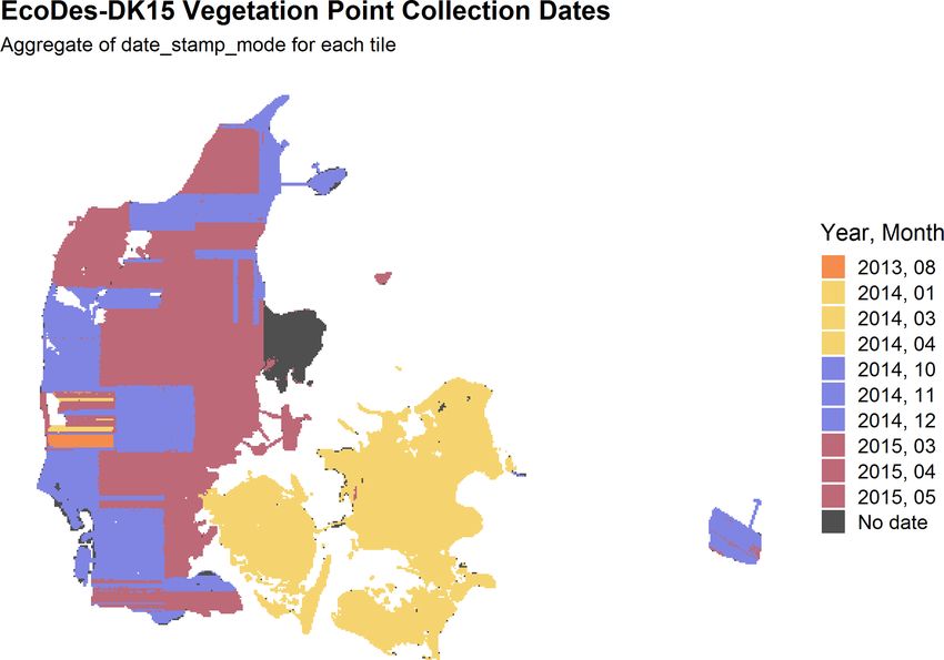
J. J. Assmann et al.: EcoDes-DK15: high-resolution ecological descriptors of vegetation and terrain                                     827

Figure 1. Diagram of the processing workflow, the dk_lidar Python module and helper scripts. The workflow requires two inputs: a pre-
classified set of point cloud tiles and a paired set of digital terrain model (DTM) tiles. The process management is handled by the pro-
cess_tiles.py script which facilitates processing of each tile pair (DTM and point cloud) in parallel and logs the progress. For each tile,
process_tiles.py calls a specified set of extraction and processing functions from the dk_lidar modules. Point cloud extraction functions
are specified in points.py and terrain model extraction functions are specified in dtm.py. The dk_lidar modules also contain two fur-
ther files: common.py, a script containing specifications of common functions used by the points.py and dtm.py,, as well as settings.py,
which is used to set global processing options, specify file paths, etc. Finally, two helper scripts are provided: progress_monitor.py, which
facilitates progress monitoring and estimates the time remaining, and debug.py, a script for testing the workflow for a single tile. To-
gether the Python scripts and modules allow the ecological descriptor outputs from the two input data sets to be generated. Further
documentation of the dk_lidar modules and workflow scripts can be found on the GitHub repository associated with this publication:
https://github.com/jakobjassmann/ecodes-dk-lidar (last access: 5 January 2022).

be found in “dtm_10m/dtm_10m_6239_446.tif”. The excep-                   named empty_tiles_XXX.txt, where XXX is the descriptor
tions are the point counts, vegetation proportions and point             name).
source information; please see the relevant sections below
for more detail.                                                         3.4     Elevation-model-derived descriptors
                                                                         The following descriptors were solely derived from the 0.4 m
                                                                         digital elevation model (DHM/Terrain). Visualisations of
3.3   Completeness of the data set                                       these descriptors for an example tile in the Mols Bjerge area
                                                                         are shown in Fig. 2.
The processing of the data set was almost completely suc-
cessful. Processing failed on average for only 18 out of the
49 673 tiles per descriptor with a maximum of 65 tiles fail-             3.4.1    Elevation (dtm_10m)
ing for the canoy_height, normalized_z_mean and normal-                  We aggregated the 0.4 m DEM by mean to match the 10 m ×
ized_z_sd descriptors. The majority of these tiles were lo-              10 m national grid of the remainder of the data set. We used
cated on the fringes of the data set, including sand spits, sand-        gdalwarp to carry out the aggregations. Values represent the
banks etc. We therefore did not attempt to re-process those              elevation above sea level in metres (DVR90, EPSG: 5799)
tiles. Instead, we generated NoData rasters for all missing              multiplied by a factor of 100, rounded to the nearest integer
descriptor–tile combinations (i.e. we assigned −9999 to all              and converted to 16 bit integer.
cells in those tiles). We provide a text file listing the affected
“NoData” tiles in the folder of each descriptor (the file is

https://doi.org/10.5194/essd-14-823-2022                                                    Earth Syst. Sci. Data, 14, 823–844, 2022
828                               J. J. Assmann et al.: EcoDes-DK15: high-resolution ecological descriptors of vegetation and terrain

Table 2. Brief overview of the 18 main EcoDes-DK15 descriptors and descriptor groups, their ecological meaning, unit, format and conver-
sion factor. See Sect. 3.4 for a detailed description of each descriptor. In addition to the 70 raster layers for the main descriptors, the data
set contains 9 layers of auxiliary information (see Sect. 3.7). Note: to obtain the correct unit, the descriptor value needs to be divided by the
conversion factor.

  Descriptor(s)                      Ecological meaning                        Unit                                 Format                             Conversion                        Number
                                                                                                                                                       factor                            of layers
  dtm_10m                            Elevation                                 m                                    16 bit integer                     100                               1
  aspect                             Topographic aspect                        Degrees                              16 bit integer                     10                                1
  slope                              Topographic slope                         Degrees                              16 bit integer                     10                                1
  heat_load_index                    Proxy of radiation and wet-               Unitless                             16 bit integer                     10 000                            1
                                     ness
  solar_radiation                    Solar radiation                           MJ ×100−1 m−2 yr−1                   32 bit integer                     1                                 1
  openness_mean                      Topographic position                      Degrees                              16 bit integer                     1                                 1
  openness_difference                Presence of linear land-                  Degrees                              16 bit integer                     1                                 1
                                     scape features
  twi                                Topographic wetness                       Unitless                             16 bit integer                     1000                              1
  amplitude_mean                     Complexb                                  Undefined                            32 bit float                       1                                 1
  amplitude_sd                       Complexb                                  Undefined                            32 bit float                       1                                 1
  canopy_height                      Vegetation height                         m                                    16 bit integer                     100                               1
  normalized_z_mean                  Average structural height                 m                                    16 bit integer                     100                               1
                                     (incl. vegetation and build-
                                     ings)
  normalized_z_sd                    Variation in structural                   m                                    16 bit integer                     100                               1
                                     height (incl. vegetation and
                                     buildings)
  point_countsa                      Number of returns in                      Count                                16 bit integer                     1                                 30
                                     ground, water, building and
                                     vegetation point classes;
                                     total return count and
                                     vegetation return counts in
                                     height bins
  vegetation_proportiona             Proportion of vegetation re-              Proportion                           16 bit integer                     10 000                            24
                                     turns in height bins
  vegetation_density                 Ratio of vegetation returns               Proportion                           16 bit integer                     10 000                            1
                                     to total returns
  canopy_openness                    Ratio of ground and water                 Proportion                           16 bit integer                     10 000                            1
                                     returns to total returns
  building_proportion                Ratio of building returns to                                                   16 bit integer                     10 000                            1
                                     total returns

  point_source_infoa                 Point source/flight strip in-             Varied, see description              Varied, see description            Varied, see description           4
                                     formation
  masks                              Inland water and sea mask                 Binary                               16 bit integer                     1                                 2
  date_stampa                        Min, max and mode of                      Date as YYYYMMDDc                    32 bit integer                     1                                 3
                                     GPS dates for all vegetation
                                     points
a Descriptor group containing multiple individual descriptors; see in-text description for detail. b The amplitude descriptors are difficult to interpret but can serve as useful indicators for
vegetation classification and biodiversity studies. Please see in-text description for more detail. c YYYY = year in four digits, MM = month in two digits, DD = day in two digits.

3.4.2      Aspect (aspect)                                                                            were carried out using gdaldem binaries and the “aspect” op-
                                                                                                      tion, which by default uses Horn’s method to calculate the
The topographic aspect describes the orientation of a slope in                                        aspect (Horn, 1981). To avoid edge effects, all calculations
the terrain and may, amongst other things, be related to plant                                        were done on a mosaic that included the focal tile and all
growth through light and moisture availability. We calculated                                         available directly neighbouring tiles (maximum eight). The
the aspect in degrees, with 0◦ indicating north, 90◦ east, 180◦                                       mosaic was cropped back to the extent of the focal tile upon
south and 270◦ west. Values represent the aspect derived                                              completion of the calculations. We then converted the value
from a 10 m aggregate of the elevation model (aggregated                                              for each cell from radians to degrees, multiplied it by a factor
by mean with 32 bit floating point precision). Calculations

Earth Syst. Sci. Data, 14, 823–844, 2022                                                                                        https://doi.org/10.5194/essd-14-823-2022
J. J. Assmann et al.: EcoDes-DK15: high-resolution ecological descriptors of vegetation and terrain 829
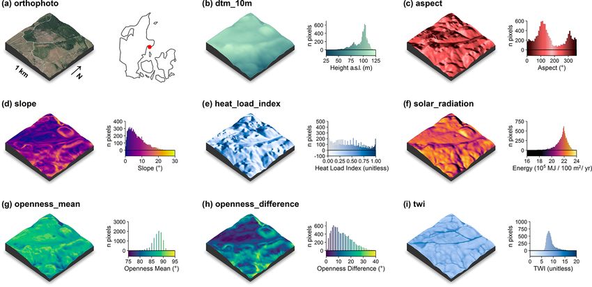
Figure 2. Illustration of the terrain-model-derived descriptors for a 1 km×1 km tile in the Mols Bjerge area (tile id: 6230_595). An orthophoto
and the tile location relative to Denmark are shown in (a). The terrain model (dtm_10m) is illustrated in (b). The terrain-derived descriptors
are comprised of (c) the topographic aspect, (d) the topographic slope, (e) the heat load index following McCune and Keon (2002), (f) the
estimated incident solar radiation, (g) the landscape openness mean, (h) the landscape openness difference in the eight cardinal directions
and (i) the topographic wetness index (TWI) based on Kopecký et al. (2020). For visualisation purposes, we amplified the altitude above
sea level by a factor of 2 in the three-dimensional visualisations and divided the solar radiation values by 105 . The three-dimensional raster
visualisations were generated using the rayshader v0.19.2 package in R (Morgan-Wall, 2020). Orthophoto provided by the Danish Agency
for Data Supply and Efficiency (https://sdfe.dk/hent-data/fotos-og-geodanmark-data/, last access: 28 June 2021).
of 10, rounded to the nearest integer and stored the results as gregate of the elevation model (32 bit floating point preci-
a 16 bit integer. Finally, we assigned a value of −10 (−1◦ ) to sion) using the gdaldem binaries with the “slope” option,
all cells where the slope was 0◦ (flat). Limitations in the as- which by default use Horn’s method to calculate the slope
pect arise in relation to edge effects that occur where a neigh- (Horn, 1981). To avoid edge effects, we carried out the cal-
bourhood mosaic is incomplete for a focal tile (i.e. less than culations on a mosaic including the focal tile and all avail-
eight neighbouring tiles), such as for tiles along the coastline able directly neighbouring tiles (maximum eight). The mo-
or at the edge of the covered extent. For those tiles, no aspect saic was cropped back to the extent of the focal tile upon
can be derived for the rows or columns at the edge of the completion of the calculations. The value for each cell was
mosaic. The cells in those rows and columns have no neigh- converted from radians to degrees, multiplied by a factor of
bouring cells and were assigned the NoData value (−9999). 10, rounded to the nearest integer and stored as a 16 bit inte-
Please also note that we calculated the aspect descriptor from ger. Limitations in the slope arise in relation to edge effects
the 10 m aggregate of the DTM/Terrain data set rather than that occur where a neighbourhood mosaic is incomplete for
deriving it from the 0.4 m original-resolution rasters and then a focal tile (i.e. less than eight neighbouring tiles), such as
aggregating it. The latter approach could represent the aspect for tiles along the coastline or at the edge of the covered ex-
at the original resolution better (Grohmann, 2015; Moudrý tent. For those tiles, no slope can be derived for the rows or
et al., 2019), but would create inconsistencies within how columns at the edge of the mosaic. These cells in those rows
the remaining DTM/Terrain descriptors are calculated in this and columns have no neighbouring cells, and gdaldem as-
data set. signs the NoData value (−9999) to these cells. Please also
note that we calculated the slope descriptor from the 10 m
aggregate of the DTM/Terrain data set rather than deriving
3.4.3 Slope (slope)
it from the 0.4 m original-resolution rasters and then aggre-
The topographic slope describes the steepness of the terrain gating it. The latter approach could represent the slope at the
and amongst other things may be related to moisture avail- original resolution better (Grohmann, 2015; Moudrý et al.,
ability, exposure and erosion. We derived the topographic 2019), but would create inconsistencies within how the re-
slope in degrees with a 10 m grain size from a mean ag-
https://doi.org/10.5194/essd-14-823-2022 Earth Syst. Sci. Data, 14, 823–844, 2022830 J. J. Assmann et al.: EcoDes-DK15: high-resolution ecological descriptors of vegetation and terrain
maining DTM/Terrain descriptors are calculated in this data hood (max. eight neighbouring tiles) to reduce edge effects
set. in subsequent calculations. We then calculated the minimum
and maximum of the positive landscape openness from all
3.4.4 Landscape openness mean (openness_mean)
eight cardinal directions for all cells in the mosaic using the
OPALS Openness module with a search radius of 50 m (fea-
Landscape openness is a landform descriptor that indicates ture = “positive”, kernelSize = 5, selMode = 1 for minimum
whether a cell is located in a depression or elevation of and selMode = 2 for maximum). Next, we converted the min-
the landscape. We calculate the landscape openness follow- imum and maximum values from radians to degrees and cal-
ing Yokoyama (2002) using the OPALS implemented algo- culated the difference between the maximum and minimum
rithms. We used a mean aggregate of the elevation model value. We rounded the result to the nearest full degree. For
with 10 m grain size and 32 bit floating point precision and the cases where the neighbourhood mosaic was incomplete,
derived the mean landscape openness for a cell as the mean i.e. containing less than eight neighbouring tiles, we masked
of the landscape openness in all eight cardinal directions with out all cells within the first 50 m of all edges with a miss-
a search radius of 150 m. We chose to base this descriptor on ing neighbourhood tile. The final output mosaic was then
the aggregated 10 m elevation model and a 150 m search ra- cropped to the extent of the focal tile and stored as a 16 bit in-
dius as we think that these are best suited to describe the teger GeoTIFF. As a consequence of the edge-effect-related
landscape-scale variation in the landforms of Denmark. Dan- masking, focal tiles on the edges of the data set, such as those
ish landscapes are characterised by gently undulating terrain, on coastlines or at the edge of the coverage area, have no data
valleys forged by small to medium sized rivers and dune sys- available for the first 50 m.
tems along the coastlines. First, we generated a mosaic in-
cluding the focal tile and all available tiles in the direct neigh- 3.4.6 Solar radiation (solar_radiation)
bourhood (max. eight neighbouring tiles) to reduce edge ef-
fects in subsequent calculations. The mean of the positive Incident solar radiation is a key parameter for plant growth
openness for all eight cardinal directions with search radius as it represents the electromagnetic energy available to plants
of 150 m was then derived for all cells in the mosaic using required for photosynthesis. However, in the comparatively
the OPALS Openness module (options: feature = “positive”, flat country of Denmark, shading by other vegetation likely
kernelSize = 15 and selMode = 0). Next, the mean openness exerts a larger influence on photosynthetic activity than
per cell was converted from radians to degrees, rounded to terrain-related shading. Here, the impact of incident solar ra-
the nearest integer and stored as a 16 bit integer. For incom- diation on the local climate likely plays a more important
plete neighbourhood mosaics (i.e. containing less than eight role for determining plant growth due to its influence on
neighbouring tiles) we then masked out cells within the first drought and water dynamics (Moeslund et al., 2019). We es-
150 m of all edges where a neighbourhood tile was missing. timated the amount of incident solar radiation received per
Finally, the output was cropped back to the extent of the fo- cell (100 m2 ) per year from the slope and aspect computed
cal tile. As a consequence of the edge-effect-related masking, as described above. Calculations were implemented using
the focal tiles on the fringes of the data set, such as those on gdal_calc, following Eq. (3) specified in McCune and Keon
coastlines or at the edge of the coverage area, have no data (2002):
available for the first 150 m. The corresponding cells for the
affected areas are set to the NoData value −9999. solar_radiation = 106
× e0.339+0.808×cos(L)×cos(S)−0.196×sin(L)×sin(S)−0.482×cos(180−|(180−A)|)×sin(S) ,
3.4.5 Landscape openness difference (1)
(openness_difference)
where L is the centre latitude of the cell in degrees, S
In addition to the mean of the landscape openness, we also is the slope of the cell in degrees, and A is the aspect
derived a landscape openness difference measure. This dif- of the cell in degrees. The resulting estimate is given in
ference measure is an indicator of whether a cell is part of a MJ × 100−1 m−2 yr−1 (McCune and Keon, 2002). Slope and
linear feature in the landscape that runs in one cardinal direc- aspect for each 10 m × 10 m grid cell were sourced from the
tion, such as a ridge or valley, therefore providing additional slope and aspect rasters. We saved the result as 32 bit inte-
information to the landscape openness_mean descriptor. We gers. Due to propagation from the calculation of slope de-
calculated the landscape openness difference based on the scriptor, no solar radiation values can be calculated for cells
10 m mean aggregate of the elevation model (32 bit floating found right on the edge of the data set, for example in tiles
point precision) and with a search radius of 50 m. We chose situated along the coastline or at the edge of the sampling
these parameters as we consider them best suited to capture extent.
the relatively narrow valleys and ridgetops common in the
Danish landscape. First, we generated a mosaic including
the focal tile and all available tiles in the direct neighbour-
Earth Syst. Sci. Data, 14, 823–844, 2022 https://doi.org/10.5194/essd-14-823-2022J. J. Assmann et al.: EcoDes-DK15: high-resolution ecological descriptors of vegetation and terrain 831
3.4.7 Heat load index (heat_load_index) 19 (Gruber and Peckahm, 2008; Quinn et al., 1991). Fourth,
we calculated the slope based on the sink-filled neighbour-
The heat load index (McCune and Keon, 2002) was origi-
hood mosaic of the terrain model (from step one) using the
nally developed as an indicator for temperature based solely
ta_morphometry 0 module with option “METHOD 7” (Har-
on aspect, but this characteristic is probably better captured
alick, 1983). Finally, we derived the TWI based on the spe-
in our solar radiation descriptor (see above) that was devel-
cific catchment area (from step three) and slope (from step
oped to improve shortcomings in the heat load index (Mc-
four) using the module ta_hydrology 20 (Beven and Kirkby,
Cune and Keon, 2002). However, in a previous study (Moes-
1979; Böhner and Selige, 2006; Moore et al., 1991). For de-
lund et al., 2019) we show that – in Denmark – the index was
tailed descriptions of the modules used, please refer to the
moderately correlated with soil moisture and can therefore
SAGA GIS documentation (SAGA-GIS Tool Library Docu-
serve as a useful indicator of the amount of moisture avail-
mentation v7.8.2, 2021).
able to plants. We calculated the heat load index based on
The TWI descriptor calculated for EcoDes-DK15 is sub-
the aspect rasters (described above) following the equation
ject to two main limitations: edge effects and small catch-
specified in McCune and Keon (2002) using gdal_calc:
ment size. Tiles with incomplete neighbourhoods (i.e. less
(1 − cos(A − 45)) than eight direct neighbours are available) will suffer from
heat_load_index = , (2)
2 edge effects in the direct vicinity of the relevant border and
where A is the aspect in degrees. We stretched the result by overall due to a reduced catchment size. Furthermore, even
a factor of 10 000, rounded to the nearest integer and stored in the ideal case of the neighbourhood being complete, for
it as a 16 bit integer. As the heat_load_index is not mean- most cells flow accumulation is therefore only calculated
ingfully defined for flat cells (slope = 0◦ / aspect = −1◦ ), we for the direct neighbourhood of a focal tile, comprising a
set the value of those cells to NoData (−9999). Finally, for 3 km × 3 km catchment area. While we hypothesise that, due
cells that are located on the outermost edges of the data set to the relatively low variation in topography in Denmark, the
the heat_load_index is not defined due to propagation of the TWI based on this comparably small catchment area will
NoData value assigned to the aspect in those cells. serve as a reasonable proxy for terrain-based wetness in most
cases, it may be less reliable in areas with exceptionally high
variation in topography or for lakes and rivers with large
3.4.8 Topographic wetness index (TWI)
catchments. In addition, we would like to point the reader
The topographic wetness index (TWI) provides a proxy mea- towards the general limitations of the TWI as a proxy for
sure of soil moisture or wetness based on the hydrolog- soil moisture or terrain wetness as, for example, discussed
ical flow modelled through a digital terrain model. Here, by Kopecký et al. (2020). These general limitations should
we derived the TWI following the method recommended by be taken into account when interpreting the TWI values pro-
Kopecký et al. (2020). We based our calculations on the ag- vided in EcoDes-DK15.
gregated 10 m elevation model (dtm_10m, 16 bit integer) and
used a neighbourhood mosaic (max. 8 neighbours) for each 3.5 Point-cloud-derived descriptors
focal tile to derive the TWI. The exact procedure is detailed
in the next paragraph. As such the index values calculated The DHM/Point-cloud point cloud was pre-classified into
by us only consider a catchment the size of one tile and all 11 point categories (Geodatastyrelsen, 2015) following the
its neighbours (for non-edge tiles this is a 3 km × 3 km catch- ASPRS LAS 1.3 standard (ASPRS, 2011). For the EcoDes-
ment, and for edge tiles it is smaller depending on the com- DK15 data set, we restricted the analysis to six of these
pleteness of the neighbourhood mosaic). We then cropped the classes, including ground points (“Terræn”) – class 2, water
resulting output back to the extent of the focal tile, stretched points (“Vand”) – class 9, and building points (“Bygninger“)
the TWI values by a factor of 1000, rounded to the next full – class 6, as well as low (“lav”), medium (“mellemhøj”) and
integer and stored the results as a 16 bit integer. high vegetation (“høj vegetation”) – classes 3, 4 and 5, re-
We calculated the TWI using SAGA GIS v. 7.8.2 bina- spectively. We grouped the three vegetation classes into one
ries. First, we sink-filled the neighbourhood mosaic of the single vegetation class and, instead of the pre-assigned height
terrain model using the ta_preprocessor 5 module and the categories, considered a more detailed set of height bins (see
option “MINSLOPE 0.01” (Wang and Liu, 2006). Second, point-count and proportion descriptions below). The overall
we calculated the flow accumulation based on the sink-filled classification accuracy of the point cloud was assessed by the
neighbourhood mosaic of the terrain model (from step one) Danish authorities (Flatman et al., 2016), but limited infor-
using the ta_hydrology 0 module with options “METHOD mation is available for the accuracy in each class. Thus, some
4” and “CONVERGENCE 1.0” (Freeman, 1991; Quinn et degree of noise should be assumed across all classes. The tall
al., 1991). Third, we derived the flow width and specific vegetation category (class 6) was used as a catch-all class if
catchment area based on the sink-filled neighbourhood mo- classification failed, as often the case for very tall buildings
saic of the terrain model (from step one) and the flow ac- and structures (Flatman et al., 2016). To reduce the noise re-
cumulation (from step two) using the module ta_hydrology lated to such structures, we removed vegetation points with
https://doi.org/10.5194/essd-14-823-2022 Earth Syst. Sci. Data, 14, 823–844, 2022832 J. J. Assmann et al.: EcoDes-DK15: high-resolution ecological descriptors of vegetation and terrain
a normalised height exceeding 50 m above ground when cal- sulting canopy heights were multiplied by a factor of 100,
culating the vegetation point counts. We included all returns, rounded to the nearest integer and stored as 16 bit integers.
i.e. first returns and echoes, in our analysis. In cases where there were no vegetation points in any given
All point cloud processing was carried out using OPALS cell, we set the canopy height value of the cell to 0 m. Please
and the OPALS Python bindings. As none of the point-cloud- note that the canopy height is therefore also set as 0 m even
derived descriptors required mosaicking to prevent edge ef- if there are no points present in the cell at all (such as ground
fects, we processed all point cloud descriptors on the focal or water points). Furthermore, our algorithm calculates the
tile only. After the initial ingestion of the LAZ file for a tile canopy height even if there is only a small amount of vege-
into the OPALS data manager format (odm), we used the tation points in a cell. In rare cases, this might lead to erro-
OpalsAddInfo module to add a normalised height (z) attribute neous canopy-height readings if vegetation is found on arti-
to the points. For this attribute we subtracted the height of the ficial structures or points have been misclassified. For exam-
ground derived from the corresponding DHM/Terrain raster ple, a tall communications tower can be found just south of
(0.4 m grid size) from the height above sea level of each Aarhus, and returns from the tower were miss-classified as
point. Figure 3 illustrates how the point cloud data trans- vegetation. The resulting canopy height for this cell is calcu-
lates to some of the descriptor outputs for four exemplary lated as > 100 m above ground, which would not make sense
10 m × 10 m cells from the data set, and an overview of the if interpreted as a height of the vegetation above ground. For
point-cloud-derived descriptors for a 1 km×1 km tile in Vejle such cases, the building proportion descriptor may be used to
Fjord in central Jutland is provided in Fig. 4. separate cells with artificial structure from those with vege-
tation only. See also the “normalized_z” descriptor below for
3.5.1 Amplitude – mean and standard deviation
a closely related measure.
(amplitude_mean and amplitude_sd)
3.5.3 Normalised height – mean and standard deviation
The amplitude attribute of a point in the DHM/Point-cloud (normalized_z_mean and normalized_z_sd)
is the actual amplitude of the return echoes; i.e. it describes
the strength of the lidar return signals detected by the sensor. Similar to the canopy height descriptor, the normalised
The descriptor is difficult to interpret in terms of its ecolog- height describes the structure properties of the point cloud
ical meaning. Nonetheless, we believe that it is still useful above ground. The key difference between the two descrip-
for vegetation classifications, biodiversity analysis and other tors is that for the normalised height we also included non-
applications that perform well with proxy data. We calculate vegetation points (buildings and ground) and derived the
the arithmetic mean and standard deviation of the amplitude summary statistic as the mean rather than the 95 % quantile.
for all points within a 10 m × 10 m cell. Here, “all points” For the normalised height descriptor, we also provide a mea-
refers to all points classified as ground, water, building and sure of variation in form of the standard deviation. Specif-
vegetation points. Calculations were carried using the OPALS ically, we calculated the normalised mean and the standard
Cell module, and results were stored as 32 bit floats. The am- deviation of the mean height above ground (normalised z
plitude attributes in the DHM/Point-cloud point clouds are attribute) for all points in each 10 m × 10 m grid cell using
not directly comparable when points originate from differ- the OPALS Cell module. The results were multiplied by 100,
ent point sources (e.g. flight strips), as the amplitude has rounded to the nearest integer and stored as 16 bit integers.
not been calibrated and hence is sensitive to differences in We used the normalised z attribute generated during the in-
sensor, sensor configuration and signal processing. Calcu- gestion of the point cloud reflecting the height of a point
lating summary metrics such as mean and standard devia- relative to the ground level determined by the DHM/Terrain
tion for a 10 m × 10 m cell where points from different point raster. Here, all points refer to all points belonging either to
sources are present introduces additional complexities. In the ground, water, building or vegetation class. By definition
some cases, a 10 m cell might contain points from up to four the normalised height mean will be highly correlated with
different sources. We therefore recommend using the two the “canopy_height” descriptor for cells where mainly veg-
amplitude descriptors with care and – if possible – in con- etation points are present. We kept the American spelling of
junction with information on the point source ids contained the descriptor name for legacy reasons with previous versions
in the point_source_info descriptors described below. of the data set.
3.5.2 Canopy height (canopy_height) 3.5.4 Point counts (xxx_point_count_xxx)
Canopy height is a key parameter of vegetation structure re- The point-count descriptors are intermediate descriptors used
lated to biomass and ecosystem functioning. We derived the to generate the proportion descriptors described below. How-
canopy height in metres as the 95th percentile of the nor- ever, they can also be used to calculate tailored proportion
malised height above ground of all vegetation points within descriptors relevant to addressing a specific ecological objec-
each 10 m × 10 m cell using the OPALS Cell module. The re- tive (see use-case example in Sect. 4.2). For EcoDes-DK15
Earth Syst. Sci. Data, 14, 823–844, 2022 https://doi.org/10.5194/essd-14-823-2022J. J. Assmann et al.: EcoDes-DK15: high-resolution ecological descriptors of vegetation and terrain 833 Figure 3. Point cloud examples for four 10 m × 10 m cells and a selection of the associated EcoDes-DK15 descriptors derived from the point clouds, illustrating the ecological meaning and some of the limitations of the EcoDes-DK15 data set. The 10 m × 10 m cells represent the following environments: (a) an agricultural field, (b) the edge of a forest/parkland pond with low vegetation, (c) a young plantation of dense coniferous trees and (d) old growth mixed woodland. The EcoDes-DK15 descriptors shown include (from the top) the total point counts for each cell in the three main EcoDes-DK15 categories: (1) the number of returns classified as ground, (2) the number of returns classified as water and (3) the number of returns classified as vegetation. In addition, the relative proportion of vegetation points per predefined height bin is illustrated below the total vegetation point count. Finally, the bottom three panels show the estimated canopy height (altitude above ground for the 95 % percentile of all vegetation returns), the normalised z standard deviation (variation in height above ground for all return classes) and the mean return amplitude for each cell. Please note how the classification of the point cloud does not separate between very low-growing vegetation (e.g. grass) and ground points in the agricultural field shown in (a), as well as how returns from water are only registered in shallow areas close to the water body’s edge, as exemplified by the forest pond in (b). Lastly, we would like to point the reader to the general limitations of ALS in penetrating forest canopies such as those shown in (c) and (d). While the upper layers of the canopies are well resolved in both cases, the laser scanning struggles to capture some aspects of the lower layers; the ground returns were frequently blocked by the thick canopy in (c), and the laser fails to meaningfully characterise understorey vegetation and stems in (d). we derived 30 point-count descriptors for each 10 m × 10 m point counts separated in height bins (Table 4). Note that the cell based on filtering of the pre-defined point classifications number of returns within a 10 m cell is influenced by (a) the and separation by height above ground (normalised z) us- number of point sources present in the cell, (b) the relative ing the OPALS Cell module. All point counts were stored position and distance of a cell to the point source when the as 16 bit integers. These 30 descriptors contain 6 general data were collected (i.e. to the flight path), and (c) the point point counts, including ground, water, vegetation, building sources themselves (i.e. differences between the lidar sen- and total point counts (Table 3), as well as 24 vegetation sors deployed). The absolute counts are therefore not directly https://doi.org/10.5194/essd-14-823-2022 Earth Syst. Sci. Data, 14, 823–844, 2022
834                      J. J. Assmann et al.: EcoDes-DK15: high-resolution ecological descriptors of vegetation and terrain

Figure 4. Illustration of the point-cloud-derived descriptors for a 1 km × 1 km tile along Vejle Fjord (tile id: 6171_541). An orthophoto and
the tile location relative to Denmark are shown in (a). The point-cloud-derived descriptors are comprised of (c) the mean return amplitude,
(d) the standard deviation in the return amplitude, (e) the canopy height (vegetation returns only), (f) the mean of the normalized height above
ground (all returns), (g) the mean of the normalized height (all returns), (h) the ground point count, (i) the water point count, (j) the building
point count, (k) the total point count, (l) the number of point sources (flight strips), (m) the canopy openness, (n) the vegetation density and
(o) the building proportion. Note the influence of point source overlap illustrated in (l) on some of the descriptors, for example, (g) ground
point count, (i) vegetation point count and (k) total point count (see Sect. 3.5.5 for detail). For visualisation purposes, we amplified the
altitude above sea level by a factor of 2 in the three-dimensional visualisations and divided the point counts by 1000. The three-dimensional
raster visualisations were generated using the rayshader v0.19.2 package in R (Morgan-Wall, 2020). Orthophotograph provided by the Danish
Agency for Data Supply and Efficiency (https://sdfe.dk/hent-data/fotos-og-geodanmark-data/, last access: 28 June 2021).

comparable between cells and need to be standardised first,                etation is distributed vertically within each cell of the raster.
for example by division of the total number of point counts                We calculated the proportions by dividing the vegetation
as done for the point proportion descriptors derived by us.                count for each height bin (Table 4) by the total point count
                                                                           (total_point_count_-01m-50m) within a given 10 m × 10 m
                                                                           cell. Resulting proportions were multiplied by a factor of
3.5.5   Vegetation proportions by height bin
                                                                           10 000, rounded to the nearest integer and converted to 16 bit
        (vegetation_proportion_xxx)
                                                                           integers. All calculations were done using gdal_calc based
The vegetation proportions by height bin are amongst the key               on the respective point-count rasters (Sect. 3.3.5). The nam-
parameters in the EcoDes-DK15 data set describing vegeta-                  ing convention of the vegetation proportion descriptors “veg-
tion structure as they provide an indication of how the veg-               etation_proportion_xxx” follows the same convention as the

Earth Syst. Sci. Data, 14, 823–844, 2022                                                       https://doi.org/10.5194/essd-14-823-2022
J. J. Assmann et al.: EcoDes-DK15: high-resolution ecological descriptors of vegetation and terrain 835
Table 3. General point-count descriptors, as well as the height ranges and point classes included in each descriptor.
Descriptor name Height range Point classes
ground_point_count_-01m-01m −1 to 1 m Ground points (class 2)
water_point_count_-01m-01m −1 to 1 m Water points (class 9)
ground_and_water_point_count_-01m-01m −1 to 1 m Ground and water points (classes 2, 9)
vegetation_point_count_00m-50m 0 to 50 m Vegetation points (classes 3, 4, 5)
building_point_count_-01m-50m −1 to 50 m Building points (class 6)
total_point_count_-01m-50m −1 to 50 m Ground, water, vegetation and building points (classes 2, 3, 4, 5, 6, 9)
Table 4. Vegetation point-count descriptors divided into 24 height ing the pre-classification. Lastly, keep in mind that dense
bins. All vegetation point counts include the point classes 3, 4 and canopy layers in the upper story of the canopy will reduce
5. penetration of the light beam to the lower canopy layers. This
may result in few returns in the lower layers (for example
Descriptor name Height range Fig. 3d) even though perhaps vegetation is present in those
vegetation_point_count_00.0m-00.5m 0.0 to 0.5 m layers.
vegetation_point_count_00.5m-01.0m 0.5 to 1.0 m
vegetation_point_count_01.0m-01.5m 1.0 to 1.5 m
3.5.6 Vegetation density or total vegetation proportion
vegetation_point_count_01.5m-02.0m 1.5 to 2.0 m
(vegetation_density)
vegetation_point_count_02m-03m 2 to 3 m
vegetation_point_count_03m-04m 3 to 4 m Vegetation density is an important component of ecosys-
vegetation_point_count_04m-05m 4 to 5 m tem structure. Here, we calculated the vegetation density
vegetation_point_count_05m-06m 5 to 6 m
as the ratio between the vegetation returns across all verti-
vegetation_point_count_06m-07m 6 to 7 m
cal height bins (vegetation_point_count_00m-50m) and the
vegetation_point_count_07m-08m 7 to 8 m
vegetation_point_count_08m-09m 8 to 9 m total point count (total_point_count_-01m-50m). Calcula-
vegetation_point_count_09m-10m 9 to 10 m tions were done using gdal_calc based on the two point-
vegetation_point_count_10m-11m 10 to 11 m count rasters (Sect. 3.3.5). Results were multiplied by 10 000,
vegetation_point_count_11m-12m 11 to 12 m rounded to the nearest integer and stored as 16 bit integers. In
vegetation_point_count_12m-13m 12 to 13 m addition to the actual difference between vegetation density
vegetation_point_count_13m-14m 13 to 14 m in a cell, the vegetation_density descriptor is also influenced
vegetation_point_count_14m-15m 14 to 14 m by the canopy properties; e.g. a dense upper layer will pre-
vegetation_point_count_15m-16m 15 to 16 m vent penetration of the light beam to lower layers or even
vegetation_point_count_16m-17m 16 to 17 m the ground, and the point sources within a cell, e.g. multiple
vegetation_point_count_17m-18m 17 to 18 m
sources from different viewing angles, provide a more com-
vegetation_point_count_18m-19m 18 to 19 m
plete estimate of the vegetation density. These additional in-
vegetation_point_count_19m-20m 19 to 20 m
vegetation_point_count_20m-25m 20 to 25 m fluences are important to keep in mind when interpreting the
vegetation_point_count_25m-50m 25 to 50 m vegetation_density descriptor.
3.5.7 Canopy openness or ground and water proportion
(canopy_openness)
vegetation point-count descriptors (Table 4), whereby the
suffix “xxx” is replaced with the respective height bin. Please Canopy openness is an important ecological descriptor par-
note that height bins are spaced at 0.5 m intervals below 2 m ticularly of forest canopies, as it describes the amount of
and at 1 m intervals between 2 and 20 m. Furthermore, the light penetrating through to the levels of the canopy. To
range above 20 m is split into only two bins: 20 to 25 m and some degree the canopy openness serves as the inverse for
25 to 50 m. the vegetation density. For EcoDes-DK15, we calculated the
Given the properties of the DHM/Point-cloud we recom- canopy openness of a 10 m×10 m cell as the proportion of the
mend being cautious when interpreting differences in the ground and water points (ground_and_water_point_count_-
lower height bins. It is likely that the inaccuracies in the point 01m-01m) to the total point count (total_point_count_-01m-
cloud complicate clear separation between points less than 50m) within the cell. The raster calculations were done us-
half a metre apart. Furthermore, note that the proportions in ing gdal_calc. Results were multiplied by 10 000, rounded to
the 0–0.5 m bin are likely biased towards an underrepresen- the nearest integer and stored as 16 bit integers. Please note
tation of the vegetation proportion in this height bin due to that the same considerations as for the vegetation_density de-
challenges in separating vegetation from ground points dur- scriptor (Sect. 3.3.7) regarding canopy properties and differ-
https://doi.org/10.5194/essd-14-823-2022 Earth Syst. Sci. Data, 14, 823–844, 2022You can also read