EarthCARE Modeling Workshop 2022- Wrap-up of DAY3- JAXA/EORC
←
→
Page content transcription
If your browser does not render page correctly, please read the page content below
EarthCARE Workshop 2022, Online, Feb 16–18, 2022

EarthCARE Modeling Workshop 2022
                  – Wrap-up of DAY3 –
   K. Suzuki (AORI), R. Forbes (ECMWF), T. Michibata (Okayama U.),
H. Kawai (MRI), M. Zhao (GFDL), A. Gettelman (NCAR), C. Golaz (LLNL),
                      and J Mülmenstädt (PNNL)

                                   Rapporter: T. Michibata (tmichibata@okayama-u.ac.jp)

    Workshop Goals
    Day3 Wrap-up
    Scientific Questions and Open Discussions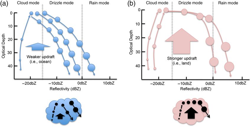
Workshop Goals (Day1–Day3)
  Key questions/issues arising from GCMs or climate modeling:
  Uncertainties of GCMs related to clouds/convection. Lessons from past COSP analysis
  on CMIP models and new initiatives.

  Analysis:
  Talks on topical analysis studies will be encouraged, including new research initiatives
  using Doppler cloud radar: e.g. global view of vertical motions/mass flux.

  Satellite simulators:
  Overview of existing satellite simulators and tasks for analysis of ECARE using
  simulators

  Assimilation:
  Assimilation is a significant part of the satellite-modeling collaboration.

  Field campaigns:
  Solidifying ECARE outcomes w/ field measurements for observations and modeling
  collaborations.

  Discussions on sciences connected to NASA/AOS (or ACCP), which is planned for
  launch around 2030, including possible collaborations with EarthCARE.
Wrap-up of DAY3 EarthCARE Workshop 2022: February 18th, 2022                           1 of 9
Day3 Agenda
  Kentaroh Suzuki (AORI/The University of Tokyo)
  Use of satellite observations for constraining aerosol-cloud-precipitation processes in
  climate models

  Science Questions:
  – How can process signatures of aerosol-cloud-precipitation interaction be identified in
    satellite observations?
  – What combination of observables? How to combine them?
  – How can they serve as metrics/diagnostics for process “fingerprint”?
  – How useful are these metrics/diagnostics to evaluate/constrain global models?
  – How do the process signatures link to macroscopic/large-scale impacts on climate?
  – How can new capabilities of EarthCARE advance model diagnostics/constraints in
    terms of these questions?

  – MODIS-CloudSat combined PDF diagram (CFODD)
  – linkage of the process realism to climate forcing
  – Dynamics-microphysics coupling from satellite? – Yes: Land / Ocean difference
  – ACI in a GCRM; how realistic

Wrap-up of DAY3 EarthCARE Workshop 2022: February 18th, 2022                           2 of 9
Day3 Agenda
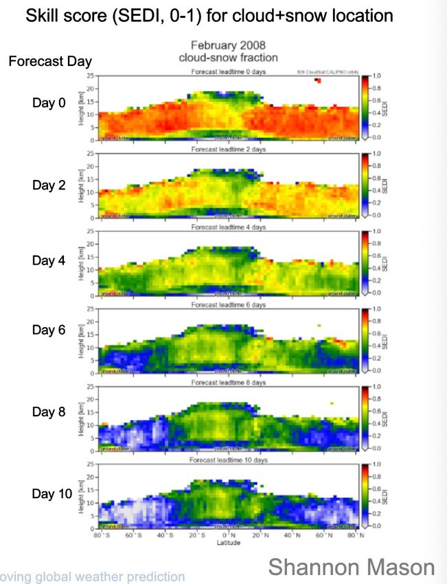
Richard Forbes (ECMWF)
Improving global weather prediction: the role of spaceborne radar and lidar
– Global NWP models – where are we heading?
– 10 DYAMOND models; There is still much uncertainty in the global characteristics of
forecast models
– Operational ECMWF global IFS 9km
– beyond 10 days; extending the forecast range
– microphysical param increasing in complexity
– multi-moment microphysical parameterization
– stochastic perturbation of total tendencies (SPPT)
– source of uncertainty in parameterization (SPP)
– Challenge: to use Doppler to constrain vertical velocity
at storm-scale
Wrap-up of DAY3 EarthCARE Workshop 2022: February 18th, 2022 3 of 9Day3 Agenda
Hideaki Kawai (MRI)
Examples of possible evaluation of GCMs using cloud radar and lidar satellite data
– cloud-top height of mid-latitude low clouds
– frequency of marine fog occurrence – CALIPSO seem well capture the fog
– various improvements in cloud processes MRI model
– SLF is improved by using CALIPSO data, contributes to well representation of
SO radiation
– improving ice fall velocity
Ming Zhao (GFDL)
A study of atmospheric river (AR), tropical storm (TS), and mesoscale convective system
(MCS) associated precipitation and extreme precipitation in present and warmer
climates
– Atmospheric river, GFDL 50 km highreso simulation
– Storm detection, Mesoscale convective systems
– % of annual precipitation from AR, TS, and MCS days
– % of extreme precipitation days also well captured
– precipitation intensity averaged from all AR, TS, and MCS days
Wrap-up of DAY3 EarthCARE Workshop 2022: February 18th, 2022 4 of 9Day3 Agenda
Andrew Gettelman (NCAR/CESM)
Confronting global models with observations of clouds and precipitation
– What are major issues for cloud and precipitation
– How can EarthCARE help?
– Model-Data fusion
– New method; machine learning
– WRF (4km) and 3km simulation with MG3 against PRISM observation
– Major issues
– cloud phase
– size distribution
– dynamics-microphysics coupling (vertical structure)
– aerosol activation (ACI)
– precipitation formation (frequency & intensity)
– SOCRATES in-situ flight over SO: CAM6 too little ice, high climate sensitivity
– dynamics
– precipitation frequency: machine learning can help to reduce precipitation bias
– to constrain microphysical relationship between Re and precipitation.
Wrap-up of DAY3 EarthCARE Workshop 2022: February 18th, 2022 5 of 9Day3 Agenda
Chris Golaz (LLNL/E3SM)
Learning from models that won’t
– E3SMv2: lower ECS and smaller ERFaci, improved against v1, but historical
temperature record
– single forcing ensemble to separate the model uncertainties
– GHG, Aerosols, Everything else (other)
– Models should understand both GHG positive forcing and negative aerosol forcing
Johannes Mülmenstädt (PNNL)
What model resolution is required to parameterize clouds, and how can observations tell
us when we’re there?
– All models are wrong, but some are useful
– negative LWP response to increased Nd from AMSR
– process fingerprints in Nd-LWP: dLWP/dt via entrainment and precipitation
– effects of turbulence on cloud adjustment
– Nd-LWP funny relation in CMIP6; why?
Wrap-up of DAY3 EarthCARE Workshop 2022: February 18th, 2022 6 of 9Summary and Next Steps
Advances in Observations
– new variables in ECARE (e.g., doppler velocity, lidar ratio)
– vertical motion, ice particle types, aerosol types (Day 1: H. Okamoto)
– improved detection sensitivity, better detection of optically thin clouds
– collocated information on CF, height, and radiation (Day 2: J.-L. Dufresne)
Advances in Modeling and Evaluation
– assumption of precipitation fraction and CFAD (Day1: T. Hashino)
– ECARE in COSP (UV lidar?)
– single forcing ensemble to separate the model uncertainties (Day 3: C. Golaz)
– Nd-LWP relation: subgrid representation; resolution (Day 3: J. Mülmenstädt)
– machine-learning approach to reduce precipitation bias (Day 3: A. Gettelman)
Obs-Model Synergies
– Geophysical Variable Maps (Day2: G. Feingold)
– resolution gaps, scale-aware/definition-aware comparison
– process-oriented diagnostics; emergent constraint (Day 3: K. Suzuki)
– radar and lidar synergy to evaluate models (Day 3: R. Forbes, H. Kawai)
– subgrid heterogeneity, vertical overlap
– how to constrain future extreme precipitation change using models and present-day
satellite record? (Day 3: M. Zhao)
Wrap-up of DAY3 EarthCARE Workshop 2022: February 18th, 2022 7 of 9EarthCARE Workshop Day3: Questions
How can we improve model biases by ECARE data and
instrument simulator?
How to use Doppler velocity of the ECARE in GCMs?
Land-Ocean Differences in Warm Rain
– Dynamics-microphysics coupling from
satellite?
– Yes: Land / Ocean difference
How can process signatures of aerosol-cloud-precipitation
Figure 2. A schematic illustration describing the warm-rain formation process over (a) weaker (i.e. ocean) and (b) stronger (i.e. land) updraughts. [Colo
be viewed at wileyonlinelibrary.com].
interaction be identified in satellite observations?
an interval of 5 µm for grouping CFODDs, similar to Suzuki
et al. (2015); however, since re = 10–15 µm is a critical range
The observed land–ocean differences in CFODDs
still due to the leftover aerosol effect after binning into
of droplet size to start the coalescence process, we further split ranges of re (i.e. the distribution of re between land and
re = 10–15 µm into two groups: 10–12.5 and 12.5−15 µm. The be different within the interval of 2.5 or 5 µm). To tes
What combination of observables? How to combine them?
re = 5–10 µm CFODD distributions over land and ocean are
similar, while the distributions for re > 10 µm are different.
probability distribution functions (PDFs) of re over lan
and ocean (blue) are also grouped into five categories a
Specifically: in Figure 1 (third row). For re > 10 µm, greater con
of aerosols over land makes continental particles sligh
How do the process signatures link to macroscopic/large-scale
1. For re = 10−15 µm, over ocean (first row), the peak in the
CFODDs shifts downward into the cloud as the reflectivity
increases with optical depth (τ d ), which indicates a
than oceanic particles. However, the land–ocean diff
PDFs are very small, suggesting that the land–ocean
in CFODDs still cannot be fully explained by aerosol
impacts on climate? downward growth of drizzle particles (−15 to 0 dBZ)
by coalescence occurs from the cloud top (τ d = 0–10) to
bottom (τ d = 40–50) as highlighted by downward arrows.
difference in cloud liquid water content (LWC) can also
the CFODD structures since coalescence is sensitive
However, the land–ocean difference in LWC near
Over land, on the other hand, the CFODDs exhibits a (τ d ≤ 10) is also small (∼0.015 gm−3 in median values
maximum nearer the cloud top, and the particles are still Many previous studies showed that updraught vel
Wrap-up of DAY3 EarthCARE Workshop 2022: February 18th, 2022
gaining height as they grow (as emphasized by the upward
arrow) in clouds. 8 of 9
stronger over land than ocean in deep convection (Z
LeMone, 1980; Lucas et al., 1994), as well as in warm clDiscussion and Comments Need to discuss about including EarthCARE function to the simulator with relevant researchers Importance of impact on weather prediction (along with climate impact) Wrap-up of DAY3 EarthCARE Workshop 2022: February 18th, 2022 9 of 9
You can also read