Diagnostics for Conditional Density Models and Bayesian Inference Algorithms
←
→
Page content transcription
If your browser does not render page correctly, please read the page content below
Diagnostics for Conditional Density Models and Bayesian Inference Algorithms

          David Zhao1                  Niccolò Dalmasso1                   Rafael Izbicki2                 Ann B. Lee1

         1
             Department of Statistics & Data Science, Carnegie Mellon University, Pittsburgh, Pennsylvania, USA
                  2
                    Department of Statistics, Federal University of São Carlos (UFSCar), São Carlos, Brazil

                         Abstract                                   mative than point predictions. Indeed, in prediction settings,
                                                                    f provides a full account of the uncertainty in the outcome
                                                                    y given new observations x. Conditional densities are also
    There has been growing interest in the AI commu-                central to Bayesian parameter inference, where the posterior
    nity for precise uncertainty quantification. Condi-             distribution f (θ|x) is key to quantifying uncertainty about
    tional density models f (y|x), where x represents               the parameters θ of interest after observing data x.
    potentially high-dimensional features, are an inte-
    gral part of uncertainty quantification in prediction           Recently, a large body of work in machine learning has
    and Bayesian inference. However, it is challenging              been developed for estimating conditional densities f for all
    to assess conditional density estimates and gain in-            possible values of x, or to generate predictions that follow
    sight into modes of failure. While existing diagnos-            the unknown conditional density (see Uria et al. 2014, Sohn
    tic tools can determine whether an approximated                 et al. 2015, Papamakarios et al. 2017, Dutordoir et al. 2018,
    conditional density is compatible overall with a                Papamakarios et al. 2021 and references therein). With the
    data sample, they lack a principled framework for               advent of high-precision data and simulations, simulation-
    identifying, locating, and interpreting the nature              based inference (SBI; Cranmer et al. [2020]) has also played
    of statistically significant discrepancies over the             a growing role in disciplines ranging from physics, chem-
    entire feature space. In this paper, we present rigor-          istry and engineering to the biological and social sciences.
    ous and easy-to-interpret diagnostics such as (i) the           The SBI category includes machine-learning based methods
    “Local Coverage Test” (LCT), which distinguishes                to learn an explicit surrogate model of the posterior [Marin
    an arbitrarily misspecified model from the true                 et al., 2016, Papamakarios and Murray, 2016, Lueckmann
    conditional density of the sample, and (ii) “Amor-              et al., 2017, Chen and Gutmann, 2019, Izbicki et al., 2019,
    tized Local P-P plots” (ALP) which can quickly                  Greenberg et al., 2019].
    provide interpretable graphical summaries of distri-            Inevitably, any downstream analysis in predictive modeling
    butional differences at any location x in the feature           or Bayesian inference depends on the trustworthiness of the
    space. Our validation procedures scale to high di-              assumed conditional density model. Validating such mod-
    mensions and can potentially adapt to any type of               els can be challenging, especially for high-dimensional or
    data at hand. We demonstrate the effectiveness of               mixed-type data x. There does not currently exist a compre-
    LCT and ALP through a simulated experiment and                  hensive and rigorous set of diagnostics that describe, for all
    applications to prediction and parameter inference              values of x, the quality of fit of a conditional density model.
    for image data.
                                                                    Related work. Large AI models, such as deep generative
                                                                    autoregressive models or Bayesian networks, are typically
                                                                    fit using global loss functions like the Kullback-Leibler
1   INTRODUCTION                                                    divergence or the L2 loss [Izbicki et al., 2017, Rothfuss
                                                                    et al., 2019]. Loss functions are useful for training mod-
There has been growing interest in the AI community for             els but only provide relative comparisons of overall model
precise uncertainty quantification (UQ), with conditional           fit. Hence, a practitioner may not know whether he or she
density models playing a key role in UQ in prediction and           should keep looking for better models (using larger training
Bayesian inference. For instance, the conditional density           samples, training times, etc.), or if the current estimate is
f (y|x) of the response variable y given features x can be          “close enough”. Another line of work assesses goodness-of-
used to build predictive regions for y, which are more infor-

                       Accepted for the 37th Conference on Uncertainty in Artificial Intelligence (UAI 2021).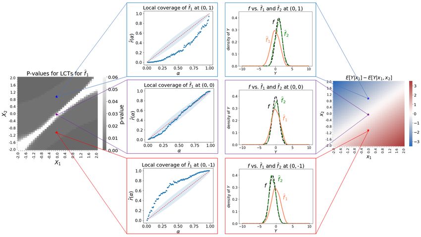
fit of a conditional density model via a two-sample test that           • [ALP - Amortized Local P-P plots] Interpretable
compare samples from fb and f . Earlier tests involve a con-              graphical summaries of the fitted model that show how
ditional version of the standard Kolmogorov test [Andrews,                it deviates from the true density at any location in fea-
1997, Zheng, 2000] in one dimension, or are tailored to spe-              ture space (see Figure 1 for examples).
cific families of conditional densities [Stute and Zhu, 2002,
Moreira, 2003]. Recently, Jitkrittum et al. [2020] developed        Our diagnostics are easy and fast to compute, and can iden-
a fast kernel-based approach that can also identify local           tify, locate, and interpret the nature of (statistically signif-
regions of poor fit. While these tests are consistent, they do      icant) discrepancies over the entire feature space. At the
                                                                    heart of our approach is the realization that the local cov-
not provide insight on how the distributions of fb and f differ
                                                                    erage of a CDE model is itself a conditional probability
locally. Kernel approaches also require the user to specify
                                                                    (see Equation 5) that often varies smoothly with x. Hence,
an appropriate kernel and tuning parameters, which can be
                                                                    we can estimate the local coverage at any given x by lever-
challenging in practice. Finally, existing diagnostics that do
                                                                    aging a suitable regression method using sample points in
describe the nature of inconsistencies between fb and f only
                                                                    a neighborhood of x. Thanks to the impressive arsenal of
test for a form of overall coherence between a data-averaged
                                                                    existing regression methods, we can adapt to different types
conditional (posterior) distribution and its marginal (prior)
                                                                    of potentially high-dimensional data to obtain computation-
distribution. Typically, they compute probability integral
                                                                    ally and statistically efficient validation. Finally, because
transform (PIT) values [Cook et al., 2006, Freeman et al.,
                                                                    we specifically evaluate local coverage (rather than other
2017, Talts et al., 2018, D’Isanto and Polsterer, 2018]. While
                                                                    types of discrepancies), the practitioner can “zoom in” on
informative, these diagnostics were originally developed for
                                                                    statistically significant local discrepancies flagged by the
assessing unconditional density models [Gan and Koehler,
                                                                    LCT, and identify common modes of failure in the fitted
1990]. As such, they are known to fail to detect some clearly
                                                                    conditional density (see Figures 4-6 for examples).
misspecified conditional models including models that ig-
nore the dependence on the covariates altogether [Schmidt
et al., 2020]. (Our Theorem 1 details different failure modes       2     EXISTING DIAGNOSTICS ARE
of existing diagnostics.)                                                 INSENSITIVE TO COVARIATE
Contribution and novelty. Our work provides diagnostic                    TRANSFORMATIONS
tools for UQ and calibration of predictive models that pro-
vide insight in simple, explainable terms like coverage, bias,      Notation. Let D = {(X1 , Y1 ), . . . , (Xn , Yn )} denote an
dispersion, and multimodality in y (output of interest) as a        i.i.d. sample from FX,Y , the joint distribution of (X, Y ) for
function of x (observed inputs). Having interpretable diag-         a random variable Y ∈ Y ⊆ R (in Section 3.3, Y is multi-
nostics is crucial for scientific collaborators and end users       variate), and a random vector X ∈ X ⊆ Rd . In a prediction
to build trust in large AI models.                                  setting, D represents a hold-out set not used to train fb. In
                                                                    a Bayesian setting, Y represents the parameter of interest
Existing diagnostics for conditional density models cannot
                                                                    (sometimes also denoted with θ), and each element of D is
detect every kind of misspecified model and give insight
                                                                    obtained by first drawing Yi from the prior distribution, and
into local quality of fit at any given x. Our method quantifies
                                                                    then drawing Xi from the statistical model of X|Yi .
deviations between actual and nominal coverage in y. It (i)
detects arbitrarily misspecified models and (ii) assesses and       Ideally, a test should be able to distinguish any given alterna-
visualizes quality of fit anywhere in feature space, even at        tive conditional density model fb(y|x) from the true density
points without observed data, in terms of easy-to-explain           f (y|x), as well as locate discrepancies in the feature space
diagnostics. To the best of our knowledge, no other method          X . More precisely, a test should be able to identify what we
in the literature provides both consistency and diagnostics         in this section define as global and local consistency.
for complex high-dimensional data.
                                                                    Definition 1 (Global Consistency). An estimate fb(y|x) is
To enrich our vocabulary for desired properties of CDEs,            globally consistent with the density f (y|x) if the following
we begin our paper by defining global and local consistency         null hypothesis holds:
(see Definitions 1 and 3, respectively). We then describe our
diagnostic framework, which has three main components:                  H0 : fb(y|x) = f (y|x) for every x ∈ X and y ∈ Y. (1)

   • [GCT - Global Coverage Test] A statistical hypoth-             Note that fb is a particular fixed conditional density estimate,
     esis test that can distinguish any misspecified density        and we test whether samples from fb are consistent with
     model from the true conditional density. (This is a test       samples from f . Existing diagnostics typically validate den-
     of global consistency.)                                        sity models by computing PIT values on independent data,
                                                                    which were not used to estimate fb(y|x):
   • [LCT - Local Coverage Test] A statistical hypothesis
     test that identifies where in the feature space the model      Definition 2 (PIT). Fix x ∈ X and y ∈ Y. The probability
     fits poorly. (This is a test of local consistency.)            integral transform of y at x, as modeled by the conditional

                       Accepted for the 37th Conference on Uncertainty in Artificial Intelligence (UAI 2021).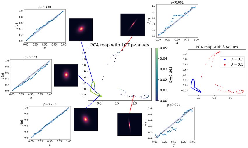
density estimate fb(y|x), is                                        Definition 3 (Local Consistency). Fix x ∈ X . An estimate
                                                                    fb(y|x) is locally consistent with the density f (y|x) at fixed
                               Z   y
                                                                    x if the following null hypothesis holds:
               PIT(y; x) =             fb(y 0 |x)dy 0 .     (2)
                               −∞
                                                                             H0 (x) : fb(y|x) = f (y|x) for every y ∈ Y.           (4)
See Figure 2, top panel for an illustration of this calculation.    In the next section, we introduce new diagnostics that are
                                                                    able to test whether a conditional density model fb is both
Remark 1. For implicit models of fb(y|x) (that is, genera-          globally and locally consistent with the underlying condi-
tive models that via e.g. MCMC can sample from, but not             tional distribution f of the data. Our diagnostics are still
directly evaluate fb), we can approximate the PIT values by         based on PIT, and hence retain the properties (e.g., inter-
forward-simulating data: For fixed x ∈ X and y ∈ Y, draw            pretability, ability to provide graphical summaries, and so
Y1 , . . . , YL ∼ fb(·|x). Then, approximate PIT(y; x) via the      on) that have made PIT a popular choice in model validation.
                         PL
cumulative sum L−1 i=1 I(yi ≤ y).

                                                                    3    NEW DIAGNOSTICS TEST LOCAL
If the conditional density model fb(y|x) is globally consis-
tent, then the PIT values are uniformly distributed. More
                                                                         AND GLOBAL CONSISTENCY
precisely, if H0 (Equation 1) is true, then the random vari-
                                          i.i.d.                    Our new diagnostics rely on the following key result:
ables PIT(Y1 ; X1 ), . . . , PIT(Yn ; Xn ) ∼ Unif(0, 1). This
result is often used to test goodness-of-fit of conditional den-    Theorem 2 (Local Consistency and Pointwise Unifor-
sity models in practice [Cook et al., 2006, Bordoloi et al.,        mity). For any x ∈ X , the local null hypothesis H0 (x) :
2010, Tanaka et al., 2018].                                         fb(·|x) = f (·|x) holds if, and only if, the distribution of
                                                                    PIT(Y ; x) given x is uniform over (0, 1).
Our first point is that unfortunately, such random variables
can be uniformly distributed even if global consistency does        Theorem 2 implies that if we had a sample of Y ’s at the fixed
not hold. This is shown in the following theorem.                   location x, we could test the local consistency (Definition
                                                                    3) of fb by determining whether the sample’s PIT values
Theorem 1 (Insensitivity to Covariate Transformations).
                                                                    come from a uniform distribution. In addition, for global
Suppose there exists a function g : X −→ Z, where Z ⊆
                                                                    consistency we need local consistency at every x ∈ X .
Rk for some k, that satisfies
                                                                    Clearly, such a testing procedure would not be practical:
                                                                    typically, we have data of the form (X1 , Y1 ), . . . , (Xn , Yn )
                    fb(y|x) = f (y|g(x)).                   (3)
                                                                    with at most one observation at any given x ∈ X .
Let (X, Y ) ∼ FX,Y . Then PIT(Y ; X) ∼ Unif(0, 1).                  Our solution is to instead address this problem as a regres-
                                                                    sion: for fixed α ∈ (0, 1), we consider the cumulative distri-
Many models naturally lead to estimates that could satisfy          bution function (CDF) of PIT at x,
the condition in Equation 3, even without being globally
consistent. In fact, clearly misspecified models fb can yield                      rα (x) := P (PIT(Y ; x) < α|x) ,                (5)
uniform PIT values and “pass” an associated goodness-of-fit         which is the regression of the random variable W           α
                                                                                                                                   :=
test regardless of the sample size. For example: if fb(y|x) is      I(PIT(Y ; X) < α) on X.
based on a linear model, then fb(y|x) will by construction
depend on x ∈ Rd only through g(x) := β T x for some                From Theorem 2, it follows that the estimated density is
                                                                    locally consistent at x if and only if rα (x) = α for every α:
β ∈ Rd . As a result, we could have fb(y|x) = f (y|g(x))
even when fb(y|x) is potentially very different from f (y|x).       Corollary 1. Fix x ∈ X . Then rα (x) = α for every α ∈
As another example, a conditional density estimator that            (0, 1) if, and only if, fb(y|x) = f (y|x) for every y ∈ Y.
performs variable selection [Shiga et al., 2015, Izbicki and
Lee, 2017, Dalmasso et al., 2020] could satisfy fb(y|x) =           Our new diagnostics are able to test for both local and global
f (y|g(x)) for g(x) := (x)S , where S ⊂ {1, . . . , d} is a         consistency. They rely on the simple idea of estimating
subset of the covariates. A test of the overall uniformity of       rα (x) and then evaluating how much it deviates from α (see
PIT values is no guarantee that we are correctly modeling           Section 3.1). Note that
the relationship between y and the predictors x; see Figure                   PIT(Y ; x) < α ⇐⇒ Y ∈ (−∞, qbα (x))
3 for an illustration.
                                                                    where qbα (x) is the α-quantile of fb. That is, rα (x) evaluates
Our second point is that current diagnostics also do not pin-       the local level-α coverage of fb at x. In Section 3.2, we ex-
point the locations in feature space X where the estimates of       plore the connection between test statistics and coverage, for
f should be improved. Hence, in addition to global consis-          interpretable descriptions of how conditional density models
tency, we need diagnostics that test the following property:
                                                                    fb may fail to approximate the true conditional density f .

                       Accepted for the 37th Conference on Uncertainty in Artificial Intelligence (UAI 2021).
3.1 LOCAL AND GLOBAL COVERAGE TESTS Algorithm 1 P-values for Local Coverage Test
Require: conditional density model fb; test data {Xi , Yi }ni=1 ;
Our procedure for testing local and global consistency is test point x ∈ X ; regression estimator rb; number of null training
very simple and can be adapted to different types of data. samples B
For an i.i.d. test sample (X1 , Y1 ), . . . , (Xn , Yn ) from FX,Y Ensure: estimated p-value pb(x) for any x ∈ X
(which was not used to construct fb), we compute Wiα := 1: // Compute test statistic at x:
I(PIT(Yi ; Xi ) < α). To estimate the coverage rα (x) (Equa- 2: Compute values PIT(Y1 ; X1 ), . . . , PIT(Yn ; Xn )
tion 5) for any x ∈ X , we then simply regress W on X 3: G ← grid of α values in (0, 1).
using the transformed data (X1 , W1 ), . . . , (Xn , Wn ). Nu- 4: for α in G do
merous classes of regression estimators can be used, from 5: Compute indicators W1α , . . . , Wnα
kernel smoothers to random forests to neural networks. 6: Train regression method rbα on {Xi , Wiα }ni=1
To test local consistency (Definition 3), we introduce the 7: end for
Local Coverage Test (LCT) with the test statistic 8: Compute test statistic T (x)
9: // Recompute test statistic under null distribution:
1 X 10: for b in 1, . . . , B do
T (x) := rα (x) − α)2 ,
(b 11:
(b) (b)
Draw U1 , . . . , Un ∼ Unif[0, 1].
|G|
α∈G 12: for α in G do
(b) (b)
where rbα denotes the regression estimator and G is a grid of 13: Compute indicators {Wα,i = I(Ui < α)}ni=1
(b) (b)
α values. Large values of T (x) indicate a large discrepancy 14: Train regression method rbα on {Xi , Wα,i }ni=1
between fb and f at x in terms of coverage, and Corollary 15: end for
1 X (b)
1 links coverage to consistency. To decide on the correct 16: Compute T (b) (x) := rα (x) − α)2
(b
cutoff for rejecting H0 (x), we use a Monte Carlo technique |G|
α∈G
that simulates T (x) under H0 . Algorithm 1 details our pro- 17: end for
B
cedure. For the LCT, note that we are performing multiple 1 X
18: return pb(x) := I T (x) < T (b) (x)
hypothesis tests at different locations x. After obtaining B
b=1
LCT p-values, we advocate using a method like Benjamini-
Hochberg to control the false discovery rate.
Similarly, we can also test global consistency (Definition 1)
with a Monte Carlo strategy. Algorithm 3 in Supp. Mat. B.
details our procedure. We introduce the Global Coverage
Test (GCT) based on the following test statistic: our work unique is that we are able to construct “amortized
n local P-P plots” (ALPs) with similar interpretations to assess
1X conditional density models over the entire feature space.
S := T (Xi ).
n i=1
Figure 1 illustrates how a local P-P plot of rbα (x) against
We recommend performing the global test first and, if the α (that is, the estimated CDF against the true CDF at x)
global null is rejected, investigating further with local tests. can identify different types of deviations in a conditional
Empirically, we have found that the power of our tests is density model. For example, positive or negative bias in the
related to the MSE (a measurable quantity) of the regression estimated density fb relative to f leads to P-P plot values
method we use. This observation is in line with similar that are too high or too low, respectively. We can also easily
results in Kim et al. [2019, Theorems 3.3 and 4.1]. Hence, identify overdispersion or underdispersion of fb from an
as a practical strategy, we maximize power by choosing the “S”-shaped P-P plot.
regression model with the smallest MSE on validation data.
Of particular note is that our local P-P plots are “amortized”,
in the sense that computationally expensive steps do not
3.2 AMORTIZED LOCAL P-P PLOTS have to be repeated with e.g Monte Carlo sampling at each
x of interest. Both the consistency tests in Section 3.1 and
Our diagnostic framework does not just give us the ability the local P-P plots only require initially training rbα on the
to identify deviations from local consistency in different observed data; the regression estimator can then be used
parts of the feature space X . It also provides us with insight to compute rbα (xval ) at any new evaluation point xval . Be-
into the nature of such deviations at any given location x. cause of the flexibility in the choice of regression method,
For unconditional density models, data scientists have long our construction also potentially scales to high-dimensional
favored using P-P plots (which plot two cumulative distri- or different types of data x. Algorithm 2 details the con-
bution functions against each other) to assess how closely a struction of ALPs, including how to compute confidence
density model agrees with actual observed data. What makes bands by a Monte Carlo algorithm.
Accepted for the 37th Conference on Uncertainty in Artificial Intelligence (UAI 2021).BIAS DISPERSION
Positive Bias Overdispersion
0.40
1.0 0.40
1.0
f f 0.8 f 0.8
0.35 0.35
0.30 0.30
0.6 0.6
r( )
r( )
0.25 0.25
0.4 0.4
0.20 0.20
f
0.15 0.15
0.10
0.2 0.10
0.2
0.0 0.0
0.05 0.05
0.00 0.25 0.50 0.75 1.00 0.00 0.25 0.50 0.75 1.00
0.00 0.00
f( |x) or f(y|x) f( |x) or f(y|x)
8 6 4 2 0 2 4 6 8 8 6 4 2 0 2 4 6 8
Negative Bias Underdispersion
0.40
1.0 0.8
1.0
f f 0.8 f 0.8
0.35 0.7
0.30 0.6
0.6 0.6
r( )
r( )
0.25 0.5
0.4 0.4
0.20 0.4
f
0.15 0.3
0.10
0.2 0.2
0.2
0.0 0.0
0.05 0.1
0.00 0.25 0.50 0.75 1.00 0.00 0.25 0.50 0.75 1.00
0.00 0.0
f( |x) or f(y|x) f( |x) or f(y|x)
8 6 4 2 0 2 4 6 8 8 6 4 2 0 2 4 6 8
Figure 1: P-P plots are commonly used to assess how well a density model fits actual data. Such plots display, in a clear and interpretable
way, effects like bias (left panel) and dispersion (right panel) in an estimated distribution fb vis-a-vis the true data-generating distribution
f . Our framework yields a computationally efficient way to construct “amortized local P-P plots” for comparing conditional densities
fb(θ|x) and fb(y|x) at any location x of the feature space X . See text for details and Sections 4-6 for examples.
Algorithm 2 Confidence bands for local P-P plot Mucesh et al. [2021] for the prediction setting. That is, the
Require: test data {Xi }ni=1 ; test point x ∈ X ; regression estima- PIT values can be computed using the estimate fb(h(Y)|x)
tor rb; number of null training samples B; confidence level η induced by fb(Y|x) for some chosen h : Rp −→ R. Differ-
Ensure: estimated upper and lower confidence bands U (x), L(x) ent projections can be used depending on the context. For
at level 1 − η for any x ∈ X instance, in Bayesian applications, posterior distributions
1: // Recompute regression under null distribution: are often used to compute credible regions for univariate
2: G ← grid of α values in (0, 1). projections of the parameters θ. Thus, it is natural to evalu-
3: for b in 1, . . . , B do ate PIT values of h(θ) = θi for each parameter of interest.
(b) (b) Another useful projection is copPIT [Ziegel and Gneiting,
4: Draw U1 , . . . , Un ∼ Unif[0, 1].
5: for α in G do 2014], which creates a unidimensional projection that has
(b) (b) information about the joint distribution of Y. Our diagnostic
6: Compute indicators {Wα,i = I(Ui < α)}ni=1
(b) (b) techniques are not enough to consistently assess the fit to
7: Train regression method rbα on {Xi , Wα,i }ni=1
f (Y|x) if applied to these projections, but they do consis-
8: end for
(b) tently evaluate the fit to f (h(Y)|x), which is often good
9: Compute rbα (x)
enough in practice.
10: end for
11: // Compute (1 − η) confidence bands for rbα (x): An alternative approach to assessing fb is through highest
12: U (x), L(x) ← ∅ predictive density values (HPD values; Harrison et al. 2015,
13: for α in G do Dalmasso et al. 2020), which are defined by
(b)
14: U (x) ← U (x) ∪ (1 − η2 )-quantile of {b
rα (x)}Bb=1 Z
15: L(x) ← L(x) ∪ η2 -quantile of {b
(b)
rα (x)}B b=1
HPD(y; x) = fb(y0 |x)dy0
y0 :fb(y0 |x)≥fb(y|x)
16: end for
17: return U (x), L(x) (see Figure 2, bottom, for an illustration). HPD(y; x) is a
measure of how plausible y is according to fb(y|x) (in the
Bayesian context, this is the complement of the e-value
3.3 HANDLING MULTIVARIATE RESPONSES [de Bragança Pereira and Stern, 1999]; small values indi-
cate high plausibility). As with PIT values, HPD values are
If the response Y is multivariate, then the random vari- uniform under the global null hypothesis [Dalmasso et al.,
able FY|X (Y|X) is not uniformly distributed [Genest and 2020]. However, standard goodness-of-fit tests based on
Rivest, 2001], so PIT values cannot be trivially generalized HPD values share the same problem as those based on PIT:
to higher dimensions. One way to overcome this is to evalu- they are insensitive to covariate transformations (see Theo-
ate the PIT statistic of univariate projections of Y, as done rem 4, Supp. Mat. A). Fortunately, HPD values are uniform
by Talts et al. [2018] for Bayesian consistency checks and under the local consistency hypothesis:
Accepted for the 37th Conference on Uncertainty in Artificial Intelligence (UAI 2021).Theorem 3. For any x ∈ X , if the local null hypothesis Shalizi [2021], we generate X = (X1 , X2 ) ∼ N (0, Σ) ∈
H0 (x) : fb(·|x) = f (·|x) holds, then the distribution of R2 , with Σ1,1 = Σ2,2 = 1 and Σ1,2 = 0.8, and take the re-
HPD(Y ; x) given x is uniform over (0, 1). (The reverse is sponse to be Y |X ∼ N (X1 + X2 , 1). To mimic the variable
however not true.) selection procedure common in high-dimensional inference
methods, we fit two conditional density models: fb1 , trained
It follows that the same techniques developed in Sections only on X1 , and fb2 , trained on X. Both models are fit-
3.1 and 3.2 can be used with HPD values to check global ted using a nearest-neighbor kernel CDE [Dalmasso et al.,
and local consistency for multivariate responses, as well as 2020] with hyperparameters chosen by data splitting: we
to construct local P-P plots. (Supp. Mat. F showcases multi- use 10000 training, 5000 validation, and 200 test points.
variate extensions via HPD.) The HPD statistic is especially
appealing if one wishes to construct predictive regions with
fb as HPD values are intrinsically related to highest predic-
tive density sets [Hyndman, 1996]. HPD sets are region
estimates of y that contain all y’s for which fb(y|x) is larger
than a certain threshold (in the Bayesian case, these are
the highest posterior credible regions). More precisely, if
HPDα (x) is the α-level HPD set for y, then
HPD(y; x) < α ⇐⇒ Y ∈ HPDα (x).
Thus, by testing local consistency of fb via HPD values, we
assess the coverage of HPD sets. It should be noted, however,
that even if the HPD values are uniform (conditional on x),
it may be the case that fb 6= f .
Figure 3: Standard diagnostics for Example 1 showing histograms
Probability Integral Transform (PIT) of PIT values computed on 200 test points (with 95% confidence
bands for a Unif[0,1] distribution). Top: Results for fb1 , which has
only been fit to the first of two covariates. Bottom: Results for fb2 ,
f (y0|x) which has been fit to both covariates. The top panel shows that
standard PIT diagnostics cannot tell that fb1 is a poor approxima-
tion to f . GCT, on the other hand, detects that fb1 is misspecified
(p=0.004), while not rejecting the global null for fb2 (p=0.894).
y y0
This is a toy example where omitting one of the variables
Highest Probability Density (HPD) might lead to unwanted bias when predicting the outcome
Y for new inputs X. As an indication of this bias, we
have included a heat map (see panel (d) of Figure 4) of
f (y0|x) the difference in the true (unknown) conditional means,
E[Y |x1 ] − E[Y |x1 , x2 ] as a function of x1 and x2 . (In this
f (y0|x) f (y|x) example, the omitted variable bias is approximately the
same as the difference in the averages of the predictions
y y0 of Y when using the model fb1 versus the model fb2 at any
given x ∈ X ; see Figure 4 panels (c) and (d)). Despite the
clear relationship between Y and X2 , both fb1 (which omits
Figure 2: Schematic diagram of the construction of PIT (top
X2 ) and fb2 pass existing goodness-of-fit tests based on PIT
panel, shaded blue area) and HPD value (bottom panel, shaded
(Figure 3). This result can be explained by Theorem 1: be-
green area) for an estimated density fb evaluated at (y, x). The
cause PIT is insensitive to covariate transformations and
highlighted red intervals in the bottom panel correspond to the
fb1 (y|x) ≈ f (y|x1 ), PIT values are uniformly distributed,
highest density region (HDR) of y|x.
even though fb1 omits a key variable. The GCT, however,
detects that fb1 is misspecified (p = 0.004), while the global
4 EXAMPLE 1: OMITTED VARIABLE null (Equation 1) is not rejected for fb2 (p = 0.894).
BIAS IN CDE MODELS The next question a practitioner might ask is: “What exactly
is wrong with the fit?”. LCTs and local P-P plots can pin-
Our first example involves omitted but clearly relevant vari- point the locations of discrepancies and describe the failure
ables in a prediction setting. Inspired by Section 2.2.2 of modes. Panel (a) of Figure 4 shows p-values from local cov-
Accepted for the 37th Conference on Uncertainty in Artificial Intelligence (UAI 2021).(a) (b) (c) (d)
Figure 4: New diagnostics for Example 1. (a) P-values for LCTs for fb1 indicate a poor fit across most of the feature space. (b) Amortized
local P-P plots at selected points show the density fb1 as negatively biased (blue), well estimated at significance level α = 0.05 with barely
perceived overdispersion (purple), and positively biased (red). (Gray regions represent 95% confidence bands under the null.) (c) fb1 and
fb2 vs. the true (unknown) conditional density f at the selected points. fb1 is clearly negatively and positively biased at the blue and red
points, respectively, while the model does not reject the local null at the purple point. fb2 fits well at all three points. The difference on
average in the predictions of Y from fb1 (·|x) vs. the true distribution f (·|x) for fixed x indeed corresponds to the “omitted variable bias”
E[Y |x1 ] − E[Y |x1 , x2 ]. (Note: Panels (c) and (d) require knowledge of the true f , which would not be available to the practitioner.)
erage tests for fb1 across the entire feature space of X. The and global consistency of models. Our proposed diagnostics
patterns in these p-values are largely explained by panel (d), identify this issue and provide insight into how the omitted
which shows the difference between the conditional means variable distorts the fitted model relative to the true condi-
of Y given x1 and given x1 , x2 . The detected level of dis- tional density, across the entire feature space.
crepancy between the estimate fb1 and the true conditional
density f at a point x directly relates to the omitted vari-
able bias E[Y |x1 ] − E[Y |x1 , x2 ] = 0.8x1 − x2 : the LCT 5 EXAMPLE 2: CONDITIONAL NEURAL
p-values close to the line x2 = 0.8x1 are large (indicating DENSITIES FOR GALAXY IMAGES
no statistically significant deviations from the true model),
and p-values decrease as we move away from this line. In this example of CDE in a prediction setting, we apply neu-
ral density models to estimate the distribution of synthetic
Panel (b) of Figure 4 zooms in on a few different locations
“redshift” Z (a proxy for distance; the response) assigned to
x with local P-P plots that depict and interpret distributional
photometric or “photo-z” galaxy images X (the predictors).
deviations. At the blue point, fb1 underestimates the true
We then illustrate how our methods distinguish between
Y : we reject the local null (Equation 4), and the P-P plot
“good” and “bad” CDEs. This toy example is motivated by
indicates negative bias. Conversely, at the red point, fb1 over- the urgent need for metrics to assess photo-z probability
estimates the true Y ; we reject the local null, and the P-P density function accuracy. Diagnostics currently used by as-
plot indicates positive bias. At the purple point, fb1 is close tronomers have known shortcomings [Schmidt et al., 2020],
to f , so the local null hypothesis is not rejected. and our method is the first to properly address them.
This toy example is a simple illustration of the general Here, x represents a 20 × 20-pixel image of an elliptical
phenomenon of potentially unwanted omitted variable bias, galaxy generated by GalSim, an open-source toolkit for
which can be difficult to detect without testing for local simulating realistic images of astronomical objects [Rowe
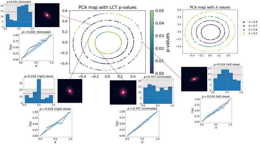
Accepted for the 37th Conference on Uncertainty in Artificial Intelligence (UAI 2021).Figure 5: New diagnostics for Example 2. For visualization, we show the location of the test galaxy points in R400 along the first two
principal components (see center panel “PCA map with LCT p-values”). Test statistics from the LCTs indicate that the unimodal density
model generally fits well for the λ = 0.8 population, while fitting poorly for the other three populations with skewed and bimodal true
redshift distributions. Local P-P plots show statistically significant deviations in the CDEs (gray regions are 95% confidence bands under
the null) for the latter population, suggesting the need for more flexible model classes.
et al., 2015]. In GalSim, we can vary the axis ratio λ, Our diagnostic framework effectively detects the flaws of
defined as the ratio between the minor and major axes of the this CDE model. First, we perform the GCT which rejects
projection of the elliptical galaxy. We create four equally the global null (p < 0.001). Next, we turn to LCTs and P-P
sized populations of galaxies, with λ ∈ {0.8, 0.7, 0.6, 0.5}. plots to explore where and how the fit is inadequate. Figure
We then assign a response variable Z according to different 5 shows a principal component map of the test data. The
distributions (unimodal, skewed and bimodal) as follows: LCTs are able to identify a unimodal Gaussian model fits
well for the λ = 0.8 population, but that the same model
Z|λ = 0.8 ∼ N (0.1, 0.02)
fails to adequately estimate the PDFs of the remaining pop-
Z|λ = 0.7 ∼ Beta(3, 7) ulations. P-P plots at selected test points indicate significant
Z|λ = 0.6 ∼ 0.6N (0.3, 0.05) + 0.4N (0.7, 0.05) distributional deviations and suggest the need to consider
Z|λ = 0.5 ∼ Beta(7, 3). more flexible model classes that incorporate bimodal and
skewed distributions.
See Figure 8 in Supp. Mat. D for a plot of these distributions.
For illustration, we fit a unimodal Gaussian neural density
model to estimate the conditional density Z|X. Our diag-
6 EXAMPLE 3: NEURAL POSTERIOR
nostics pinpoint where in the feature space the density is
bimodal or skewed, and thus a fit with one Gaussian is inad- INFERENCE FOR GALAXY IMAGES
equate. We know of no other diagnostics that can provide
such insight when fitting neural density models. Specifically, Our final example tests for image data x ∈ R400 whether
we fit a convolutional mixture density network (ConvMDN, a Bayesian posterior model fb(θ|x) fits the true posterior.
D’Isanto and Polsterer [2018]) with a single Gaussian com- As in Example 2, x represents an image of an elliptical
ponent, two convolutional and two fully connected layers galaxy generated by GalSim. As before, λ is the galaxy’s
with ReLU activations [Glorot et al., 2011]. (We train on axis ratio, but now the quantity of interest θ is the galaxy’s
10000 images using the Adam optimizer [Kingma and Ba, rotation angle with respect to the x-axis; that is, an unknown
2014] with learning rate 10−3 , β1 = 0.9, and β2 = 0.999.) internal parameter. For illustration, we create a mixture of a
This gives an estimate of f (z|x). We expect this CDE model larger population with λ = 0.7 (spheroidal galaxies), and a
to fit well for the λ = 0.8 unimodal population, and fit smaller population with λ = 0.1 (elongated galaxies). We
poorly for the other bimodal or skewed populations. then simulate a sample of images as follows: first, we draw
Accepted for the 37th Conference on Uncertainty in Artificial Intelligence (UAI 2021).Figure 6: New diagnostics for simulation-based inference algorithm in Example 3. For visualization, we show the location of the test
galaxy points in R400 along its first two components (see center panel “PCA map with LCT p-values”). P-values for LCTs indicate that
the ConvMDN generally fits well for the dominant 90% population of spheroidal galaxies (λ = 0.7), while fitting poorly for the smaller
10% subpopulation of elongated galaxies (λ = 0.1). Local P-P plots show statistically significant deviations in the CDEs (gray regions are
95% confidence bands under the null) for the latter population, suggesting we need better approximations of the posterior for this group.
λ and θ from a prior distribution given by bias in the posterior estimates for the λ = 0.1 population.
These plots suggest that an effective way of obtaining a
P(λ = 0.7) = 1 − P(λ = 0.1) = 0.9 better approximation of the posterior is by improving the
θ ∼ U nif (−π, π) fit for the λ = 0.1 population (by obtaining more data in
that region of the feature space, using a different model
Then we sample 20 × 20 galaxy images X according to the class, etc). For instance, CDE models not based on mixtures
data model X|λ, θ ∼ GalSim(a, λ), where [Papamakarios et al., 2019] could be more effective.
Conclusion. Conditional density models are widely used for
a|λ = 0.7 ∼ N (θ, 0.05)
uncertainty quantification in prediction and Bayesian infer-
a|λ = 0.1 ∼ 0.5Laplace(θ, 0.05) + 0.5Laplace(θ, 0.0005). ence. In this work, we offer practical procedures (GCT, LCT,
ALP) for identifying, locating, and interpreting modes of
As in Example 2, we fit a convolutional mixture density failure for an approximation of the true conditional density.
network (ConvMDN); in this case, it gives us an estimate Our tools can be used in conjunction with loss functions,
of the posterior distribution f (θ|x). This time, we allow K, which are useful for performing model selection, but not
the number of mixture components, to vary. According to good at evaluating whether a practitioner should keep look-
the KL divergence loss computed on a separate test sample ing for better models, or at providing information as to how
with 1000 images, the best fit of f (θ|x) is achieved by a a model could be improved. Finally, because LCT pinpoints
ConvMDN model with K = 7 (see Table 1 in Supp. Mat. E). hard-to-train regions of the feature space, our framework
Here, the ConvMDN model with the smallest KL loss fails can provide guidance for active learning schemes.
the GCT (p < 0.001), so we turn to LCTs and P-P plots to
Acknowledgments. This work is supported by NSF DMS-
understand why. Figure 6 plots the test galaxy images along
2053804 and NSF PHY-2020295. RI is grateful for the
their first two principal components. The LCTs show that the
financial support of CNPq (309607/2020-5) and FAPESP
ConvMDN model generally fits the density well for the main
(2019/11321-9).
population of spheroidal galaxies (λ = 0.7), but fails to
properly model the smaller population of elongated galaxies
(λ = 0.1). P-P plots at selected test points indicate severe
Accepted for the 37th Conference on Uncertainty in Artificial Intelligence (UAI 2021).References Christian Genest and Louis-Paul Rivest. On the multivariate
probability integral transformation. Statistics & probabil-
D. W. K. Andrews. A conditional Kolmogorov test. Econo- ity letters, 53(4):391–399, 2001.
metrica, 65(5):1097 – 1128, 1997.
Xavier Glorot, Antoine Bordes, and Yoshua Bengio. Deep
Rongmon Bordoloi, Simon J. Lilly, and Adam Amara. sparse rectifier neural networks. In Proceedings of the
Photo-z performance for precision cosmology. Monthly Fourteenth International Conference on Artificial Intel-
Notices of the Royal Astronomical Society, 406(2):881– ligence and Statistics, volume 15 of Proceedings of Ma-
895, 08 2010. doi: 10.1111/j.1365-2966.2010.16765.x. chine Learning Research, pages 315–323, Fort Laud-
erdale, FL, USA, 11–13 Apr 2011. JMLR Workshop and
Yanzhi Chen and Michael U. Gutmann. Adaptive gaus- Conference Proceedings.
sian copula ABC. In Kamalika Chaudhuri and Masashi
Sugiyama, editors, Proceedings of Machine Learning Re- David Greenberg, Marcel Nonnenmacher, and Jakob Macke.
search, volume 89 of Proceedings of Machine Learning Automatic posterior transformation for likelihood-free
Research, pages 1584–1592. PMLR, 16–18 Apr 2019. inference. In Proceedings of the 36th International Con-
ference on Machine Learning, volume 97 of Proceedings
Samantha R. Cook, Andrew Gelman, and Donald B. Rubin. of Machine Learning Research, pages 2404–2414, Long
Validation of software for Bayesian models using poste- Beach, California, USA, 09–15 Jun 2019. PMLR.
rior quantiles. Journal of Computational and Graphical
Statistics, 15(3):675–692, 2006. Diana Harrison, David Sutton, Pedro Carvalho, and Michael
Hobson. Validation of Bayesian posterior distribu-
Kyle Cranmer, Johann Brehmer, and Gilles Louppe. The
tions using a multidimensional Kolmogorov–Smirnov
frontier of simulation-based inference. Proceedings of
test. Monthly Notices of the Royal Astronomical Soci-
the National Academy of Sciences, 117(48):30055–30062,
ety, 451(3):2610–2624, 06 2015. ISSN 0035-8711. doi:
2020.
10.1093/mnras/stv1110.
Niccolò Dalmasso, Taylor Pospisil, Ann B. Lee, Rafael
Rob J. Hyndman. Computing and graphing highest density
Izbicki, Peter E. Freeman, and Alex I. Malz. Conditional
regions. The American Statistician, 50(2):120–126, 1996.
density estimation tools in Python and R with applications
to photometric redshifts and likelihood-free cosmolog-
Rafael Izbicki and Ann B. Lee. Converting high-
ical inference. Astronomy and Computing, 30:100362,
dimensional regression to high-dimensional conditional
Jan 2020. ISSN 2213-1337. doi: 10.1016/j.ascom.2019.
density estimation. Electronic Journal of Statistics, 11
100362.
(2):2800–2831, 2017.
Carlos Alberto de Bragança Pereira and Julio Michael Stern.
Rafael Izbicki, Ann B. Lee, and Peter E. Freeman. Photo-
Evidence and credibility: full Bayesian significance test
z estimation: An example of nonparametric conditional
for precise hypotheses. Entropy, 1(4):99–110, 1999.
density estimation under selection bias. Annals of Applied
Antonio D’Isanto and Kai Lars Polsterer. Photometric red- Statistics, 11(2):698–724, 2017.
shift estimation via deep learning. generalized and pre-
classification-less, image based, fully probabilistic red- Rafael Izbicki, Ann B. Lee, and Taylor Pospisil. ABC–CDE:
shifts. Astronomy & Astrophysics, 609:A111, 2018. Toward Approximate Bayesian Computation With Com-
plex High-Dimensional Data and Limited Simulations.
Vincent Dutordoir, Hugh Salimbeni, Marc Peter Deisen- Journal of Computational and Graphical Statistics, pages
roth, and James Hensman. Gaussian process conditional 1–20, 2019. doi: 10.1080/10618600.2018.1546594.
density estimation. In Advances in Neural Information
Processing Systems 31, Neural Information Processing Wittawat Jitkrittum, Heishiro Kanagawa, and Bernhard
Systems. Curran Associates, Inc., 2018. Schölkopf. Testing goodness of fit of conditional density
models with kernels. In Proceedings of the 36th Confer-
Peter E. Freeman, Rafael Izbicki, and Ann B. Lee. A unified ence on Uncertainty in Artificial Intelligence (UAI), vol-
framework for constructing, tuning and assessing photo- ume 124 of Proceedings of Machine Learning Research,
metric redshift density estimates in a selection bias setting. pages 221–230. PMLR, 03–06 Aug 2020.
Monthly Notices of the Royal Astronomical Society, 468
(4):4556–4565, 2017. doi: 10.1093/mnras/stx764. Ilmun Kim, Ann B. Lee, and Jing Lei. Global and lo-
cal two-sample tests via regression. Electronic Journal
Fah F. Gan and Kenneth J. Koehler. Goodness-of-fit tests of Statistics, 13(2):5253 – 5305, 2019. doi: 10.1214/
based on p-p probability plots. Technometrics, 32(3): 19-EJS1648. URL https://doi.org/10.1214/
289–303, 1990. doi: 10.1080/00401706.1990.10484682. 19-EJS1648.
Accepted for the 37th Conference on Uncertainty in Artificial Intelligence (UAI 2021).Diederik P. Kingma and Jimmy Ba. Adam: A method for Barnaby Rowe, Mike Jarvis, Rachel Mandelbaum, Gary M.
stochastic optimization. arXiv preprint arXiv:1412.6980, Bernstein, James Bosch, Melanie Simet, Joshua E. Mey-
2014. ers, Tomasz Kacprzak, Reiko Nakajima, Joe Zuntz, et al.
GALSIM: The modular galaxy image simulation toolkit.
Jan-Matthis Lueckmann, Pedro J. Gonçalves, Giacomo Bas-
Astronomy and Computing, 10:121–150, 2015.
setto, Kaan Öcal, Marcel Nonnenmacher, and Jakob H.
Macke. Flexible statistical inference for mechanistic S. J. Schmidt, A. I. Malz, J. Y. H. Soo, I. A. Almosallam,
models of neural dynamics. In Proceedings of the 31st M. Brescia, S. Cavuoti, J. Cohen-Tanugi, et al. Eval-
International Conference on Neural Information Process- uation of probabilistic photometric redshift estimation
ing Systems, NIPS’17, page 1289–1299, Red Hook, NY, approaches for The Rubin Observatory Legacy Survey of
USA, 2017. Curran Associates Inc. Space and Time (LSST). Monthly Notices of the Royal
Jean-Michel Marin, Louis Raynal, Pierre Pudlo, Mathieu Astronomical Society, 499(2):1587–1606, 2020.
Ribatet, and Christian Robert. ABC random forests for Cosma Shalizi. Advanced Data Analysis from an Elemen-
Bayesian parameter inference. Bioinformatics (Oxford, tary Point of View. Cambridge University Press, 2021.
England), 35, 05 2016. doi: 10.1093/bioinformatics/
bty867. Motoki Shiga, Voot Tangkaratt, and Masashi Sugiyama.
Direct conditional probability density estimation with
M. J. Moreira. A conditional likelihood ratio test for struc- sparse feature selection. Machine Learning, 100(2):161–
tural models. Econometrica, 71(4):1027 – 1048, 2003. 182, 2015. doi: 10.1007/s10994-014-5472-x.
S. Mucesh, W. G. Hartley, A. Palmese, O. Lahav, L. White-
Kihyuk Sohn, Honglak Lee, and Xinchen Yan. Learning
way, A. F. L. Bluck, A. Alarcon, A. Amon, K. Bechtol,
structured output representation using deep conditional
G. M. Bernstein, A. Carnero Rosell, M. Carrasco Kind,
generative models. In C. Cortes, N. Lawrence, D. Lee,
and DES Collaboration. A machine learning approach to
M. Sugiyama, and R. Garnett, editors, Advances in Neu-
galaxy properties: joint redshift–stellar mass probability
ral Information Processing Systems, volume 28. Curran
distributions with random forest. Monthly Notices of the
Associates, Inc., 2015.
Royal Astronomical Society, 502(2):2770–2786, 01 2021.
doi: 10.1093/mnras/stab164. W. Stute and L. X. Zhu. Model checks for generalized linear
George Papamakarios and Iain Murray. Fast -free Infer- models. Scandinavian Journal of Statistics, 29(3):535 –
ence of Simulation Models with Bayesian Conditional 545, 2002. ISSN 0303-6896.
Density Estimation. In D. Lee, M. Sugiyama, U. Luxburg, Sean Talts, Michael Betancourt, Daniel Simpson, Aki Ve-
I. Guyon, and R. Garnett, editors, Advances in Neural htari, and Andrew Gelman. Validating Bayesian infer-
Information Processing Systems, volume 29. Curran As- ence algorithms with simulation-based calibration. arXiv
sociates, Inc., 2016. preprint arXiv:1804.06788, 2018.
George Papamakarios, Theo Pavlakou, and Iain Murray.
Masayuki Tanaka, Jean Coupon, Bau-Ching Hsieh, Sogo
Masked autoregressive flow for density estimation. In
Mineo, Atsushi J Nishizawa, Joshua Speagle, Hisanori
Proceedings of the 31st International Conference on Neu-
Furusawa, Satoshi Miyazaki, and Hitoshi Murayama.
ral Information Processing Systems, NIPS’17, Red Hook,
Photometric redshifts for Hyper Suprime-Cam Subaru
NY, USA, 2017. Curran Associates Inc.
Strategic Program Data Release 1. Publications of the
George Papamakarios, David Sterratt, and Iain Murray. Se- Astronomical Society of Japan, 70(SP1), 01 2018. doi:
quential neural likelihood: Fast likelihood-free inference 10.1093/pasj/psx077.
with autoregressive flows. In 22nd International Confer-
Bengio Uria, Iain Murray, and Hugo Larochelle. A deep and
ence on Artificial Intelligence and Statistics, Proceedings
tractable density estimator. In Proceedings of the 31st In-
of Machine Learning Research, pages 837–848. PMLR,
ternational Conference on Machine Learning, volume 32
2019.
of Proceedings of Machine Learning Research, Beijing,
George Papamakarios, Eric Nalisnick, Danilo Jimenez China, 09–15 Jun 2014. JMLR.
Rezende, Shakir Mohamed, and Balaji Lakshmi-
narayanan. Normalizing flows for probabilistic modeling J. X. Zheng. A consistent test of conditional parametric dis-
and inference. Journal of Machine Learning Research, tributions. Econometric Theory, 16(5):667 – 691, 2000.
22(57):1–64, 2021. Johanna F. Ziegel and Tilmann Gneiting. Copula calibration.
Jonas Rothfuss, Fabio Ferreira, Simon Walther, and Maxim Electronic Journal of Statistics, 8(2):2619–2638, 2014.
Ulrich. Conditional density estimation with neural net- doi: 10.1214/14-EJS964.
works: Best practices and benchmarks. arXiv preprint
arXiv:1903.00954, 2019.
Accepted for the 37th Conference on Uncertainty in Artificial Intelligence (UAI 2021).You can also read