Deep parameter free attention hashing for image retrieval - Nature
←
→
Page content transcription
If your browser does not render page correctly, please read the page content below
www.nature.com/scientificreports
OPEN Deep parameter‑free attention
hashing for image retrieval
Wenjing Yang1, Liejun Wang2* & Shuli Cheng2
Deep hashing method is widely applied in the field of image retrieval because of its advantages of
low storage consumption and fast retrieval speed. There is a defect of insufficiency feature extraction
when existing deep hashing method uses the convolutional neural network (CNN) to extract images
semantic features. Some studies propose to add channel-based or spatial-based attention modules.
However, embedding these modules into the network can increase the complexity of model and lead
to over fitting in the training process. In this study, a novel deep parameter-free attention hashing
(DPFAH) is proposed to solve these problems, that designs a parameter-free attention (PFA) module
in ResNet18 network. PFA is a lightweight module that defines an energy function to measure the
importance of each neuron and infers 3-D attention weights for feature map in a layer. A fast closed-
form solution for this energy function proves that the PFA module does not add any parameters to
the network. Otherwise, this paper designs a novel hashing framework that includes the hash codes
learning branch and the classification branch to explore more label information. The like-binary codes
are constrained by a regulation term to reduce the quantization error in the continuous relaxation.
Experiments on CIFAR-10, NUS-WIDE and Imagenet-100 show that DPFAH method achieves better
performance.
Recently, a great number of media data have been extensively used in various industries such as computer vision
and network security1,2. Image retrieval in computer vision is the focus of current research. It is an urgent problem
that quickly retrieve the similar image from a large data set. Due to the advantages of fast query speed and low
storage cost, deep hashing method3–7 is widely applied in the field of image retrieval. The purpose of deep hash-
ing is to convert high-dimensional images to low-dimensional binary codes by using a hash function, thereby
preserving similar information of original images.
In the early image retrieval methods, text-based image retrieval (TBIR)8,9 follows the traditional text anno-
tation technology to implement retrieval by text matching. In content-based image retrieval (CBIR)10,11, with
the help of the computer to explore image content features and take it as clues to detect other images with
similar features from image database. However, TBIR and CBIR need a great quantity manual operation and
computational resources. On the contrary, deep hashing methods12–14 have obvious advantages by utilizing
CNN as a features extractor. Existing deep hashing are divided into data-independent and data-dependent. In
the data-independent h ashing15, the hash codes are obtained by randomly mapping matrix and the accuracy of
hash functions cannot be guaranteed. Data-dependent h ashing16,17 explore multiple aspects of images such as
shape, texture and colors to generate hash codes with discrimination ability. This study uses the data-dependent
methods to learn high-quality hash codes.
Most current hashing methods commonly use the shallow CNN to explore high-dimensional semantic fea-
tures and map them to hash codes via a hash function. However, the feature learning part of these methods have
defects that features extraction is insufficiency and imbalance. Meanwhile, the hashing learning part cannot
make full use of label information and produce insurmountable quantization errors, which significantly affect
the accuracy of hash codes. Therefore, some scholars suggest adding channel-wise and spatial-wise attention
mechanism to backbone network18,19. Such attention modules usually cause two problems. First, the flexibility of
learning attention weights is hampered because they can only extract images features along channels or spatial
dimensions. Second, their structures are composed of complicated factors, it will increase the complexity of the
training model and cause over fitting.
To optimize the above problems, this paper is encouraged by 3-D attention m odule20 and semantic hierarchy
preserving deep hashing21. This paper designs a parameter-free attention (PFA) module which defines an energy
function that consider the weights of both channel and spatial dimensions. This module makes the network learn
more differentiated neurons without adding parameters, and the high-level semantic features of the images can
be fully explored through refine those neurons. Specifically, ResNet18 is chosen as backbone network. As shown
1
College of Software, Xinjiang University, Urumqi 830046, China. 2College of Information Science and Engineering,
Xinjiang University, Urumqi 830046, China. *email: wljxju@xju.edu.cn
Scientific Reports | (2022) 12:7082 | https://doi.org/10.1038/s41598-022-11217-5 1
Vol.:(0123456789)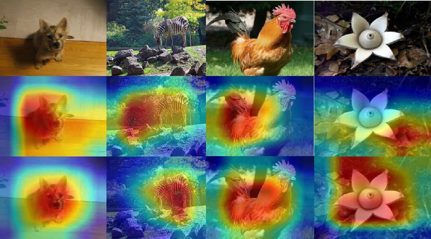
www.nature.com/scientificreports/
in Fig. 1, the whole process is mainly divided into four steps. First, the pairs of images are fed into the Convolu-
tion layer and the Maximum pooling layer to generate feature map. Second, the feature map is processed by
PFA module, which considers both the 1-D channel-wise weights and the 2-D spatial-wise weights and directly
generated 3-D weights. Third, this paper performs the operation of element-wise sum on PFA output and feature
map and input the result to the backbone network to extract image features. Finally, in order to make efficient use
of semantic label information, two branches containing classifier layer and hashing layer is designed. Combining
the pair-wise loss and quantization loss generated by the hashing layer and class-wise loss generated classifier to
obtain hash codes with discriminative ability.
In short, the contributions are as follows:
1. DPFAH is an end-to-end learning framework which perform simultaneous feature representation and
binary codes learning. A lightweight module is introduced to extract rich semantic features and avoid over
fitting in the training process.
2. The PFA module is embedded in ResNet18 network to improve the feature representation. It explores an
energy mathematical formula to calculate the 3-D weight and derives a closed-form solution that speedup
the weight calculation. No parameters are added to the network during the whole process.
3. A novel deep hashing framework is designed by DPFAH, which includes hashing learning and classifica-
tion. This method can use the label information to eliminate discrepancy and generate more accurate hash
codes. Experimental results on three datasets have verified DPFAH.
The remaining content of this paper is as follows. “Related work” is related work. “Deep Parameter-free
attention hashing” describes the details of DPFAH. “Experiments” is the results of experiments and analysis.
“Conclusions” summarizes the work of this study.
Related work
Deep learning is applied in many fields for its advantages of a solid learning ability and good portability. Network
security fields use neural networks to detect m alware22,23 and programs24, The field of artificial intelligence can
be conducive to the intelligent estimation of traffic time by deep learning methods25. This paper focuses on the
research of hashing algorithm based on deep learning. Deep hashing is widely applied in image retrieval system
due to its own advantages. For example, the function of searching images by image is realized through deep
hashing in many shopping software. Therefore, how to obtain hash code with strong accuracy for each image has
become a research hotspot. In this section, the existing several unsupervised hashing approaches and supervised
hashing approaches are introduced.
Unsupervised hashing. Unsupervised hashing26–30 only utilizes the unlabeled data points to learn hash
function that map high dimensional feature to compact hash codes. The similarity matrix is usually constructed
in the process of feature learning. Many scholars have carried a lot of study on the perspective of constructing
similarity matrix. Specifically, Sheng et al. proposed28 the descriptors of data are represented by the output of
full-connected layer and used to design the similarity matrix. The network is optimized by calculating the loss
between the similarity matrix and pairwise hash codes. By observing the law of features distribution, Yang et al.
proposed29 the cosine distance of pairs data can be evaluated by Gaussian distributions. They set a distance
threshold in the steps of constructing the similarity matrix, the data points are defined as similar if the cosine
roposed30 the cosine dis-
distance of data points smaller than threshold, vice versa. On this basis, Jiang et al. p
tance was used directly to guide the construction of similarity matrix, and encouraged by31 , they chose the
gradient attention to optimize the network. Although unsupervised hashing retrieval faces great challenges due
to without labels information, these methods contribute to the development of image retrieval.
Supervised hashing. Compared to unsupervised hashing, supervised hashing methods try to explore data
labels as supervised information to calculate similarity matrix. Early on, Xia et al. proposed32 to learn semantic
features and hash codes separately, and there is no feedback between them. Recent supervised hashing usually
designs an end-to-end learning framework to learn features and hash codes simultaneously such as31–34. On this
basis, Cao et al.18 selected a tanh activation function that make the network output is continuous hash codes.
To avoid the discrete limit imposed on like-binary codes, Su et al. proposed35 the greedy rules by updating the
parameters toward the possible optimum discrete solution. In order to solve the problem of imbalanced distribu-
tion of data labels, Jiang et al.36 introduced a soft concept that quantified pairwise similarity as a percentage by
using labels information. Meanwhile, Cao et al.37 proposed to weight the similarity matrix of training pairs and
the Cauchy distribution is utilized instead of sigmoid function to calculate the loss. These methods are improve-
ments in the loss function, but they ignore the problem of insufficient image features extraction. Hence, Li et al.19
embedded channel attention and spatial attention into CNN to obtain sufficient semantic features. Yang et al.34
improved the feature map in the dual attention module and combined it with the backbone network. However,
these modules can aggravate the complexity of the network model and affect the speed of training. Motivated
by38, this paper introduces a lightweight attention module based on ResNet18 and design a new class-wise loss,
which suitable for learning more accurate hash codes.
Deep parameter‑free attention hashing
In this section, the detail of DPFAH method is described, including research motivation, the definition of letters
and formulas, the architecture of network, PFA module and the process of optimizing network.
Scientific Reports | (2022) 12:7082 | https://doi.org/10.1038/s41598-022-11217-5 2
Vol:.(1234567890)
www.nature.com/scientificreports/
class-wise loss
Back-propagation
Classifier
Conv1 Maxpool Avgpool
Layer1 Layer4
PFA Module Pair-wise loss
Train Images +1 +1 -1 -1
-1 +1 +1 -1
Sign +1 -1 -1 +1
-1 -1 -1 +1
Hashing layer
Query Image
Hash codes Hash codes
Hashing search database DH
Return Retrieval Images DH : Hamming distance
: Element-wise sum
Figure 1. The overall framework of deep parameter-free attention hashing module, which is composed of three
parts: (1) pairs of images are fed into Convolution and Maxpool layer to obtain feature map; (2) features map is
fed into the PFA module, and the result obtained perform the element-wise sum operation with feature map; (3)
a hashing layer is designed to generate hash codes, and three loss functions are used to optimize the network.
(Created by ‘Microsoft Office Visio 2013’ url: https://www.microsoft.com/zh-cn/microsoft-365/previous-versi
ons/microsoft-visio-2013).
Research motivation. Recently, there are some defects in deep hashing method that need to be deal with:
(1) shallow network cannot fully extract the semantic feature information of images, some channel-based or
spatial-based attention modules can increase the complexity of model and lead to over fitting; (2) the process of
relaxing hash codes can produce inevitable quantization error.
In order to solve the problem of insufficient feature extraction, some scholars consider adding attention
mechanism modules to the network, which will increase the complexity of network computing and algorithm
time complexity. Based on the above considerations, the goal of this paper is to design a lightweight module that
can extract image features without adding any parameters to the network, and a regulation term constrained
hash codes is proposed to reduce the quantization error.
Problem formulation. In the similarity retrieval, given a dataset with n images are represented as
X = {xi }ni=1, where xi represents the ith image. The label of X is denoted as Y = {yi }ci=1, where yi is the labels of
the ith image and c is the number of classes. Therefore, the similarity matrix S = {sij } is defined as:
1, if xi and xj belong to the same class
sij =
0, otherwise (1)
The target of deep hashing is to learn a hash function F(θ; xi ) that project xi to bi ∈ {−1, +1}l , where θ
represents the parameters of CNN and l is the length of hash codes. Therefore, each image xi is mapped to l
-dimensional vector U = {ui }ni=1 passing through F model, where ui is the l -dimensional vector of the ith image.
To reduce quantification loss, inspired by34, ui is processed by a piecewise function as follow:
1, ui > 1
f (ui ) = ui , −1 < ui < 1 (2)
−1, ui < −1
Finally, bi = sign(f (ui )) is used to map l -dimension ui to l -bit bi , the sign(.) is defined as follow:
−1, x ≥ 0
sign(x) =
1, otherwise (3)
Network architecture. Figure 1 shows the framework of DPFAH, which includes three main parts. DFPAH
utilizes ResNet18 as backbone network, in order to fully improve the salient features representation ability and
does not increase the computational complexity of the model. This paper has drawn a simple and parameter-free
module into network, which can explore neurons in each channel or spatial location to learn more discrimina-
tive cues. In addition, the last layer of basic residual network is the classification layer that assigns data to the
same class. On this basis, the hashing branch is designed parallel to the classification branch. The class-wise loss
generated by the classification branch will positively affect the hashing branch when the parameters are updated
by back propagation.
Scientific Reports | (2022) 12:7082 | https://doi.org/10.1038/s41598-022-11217-5 3
Vol.:(0123456789)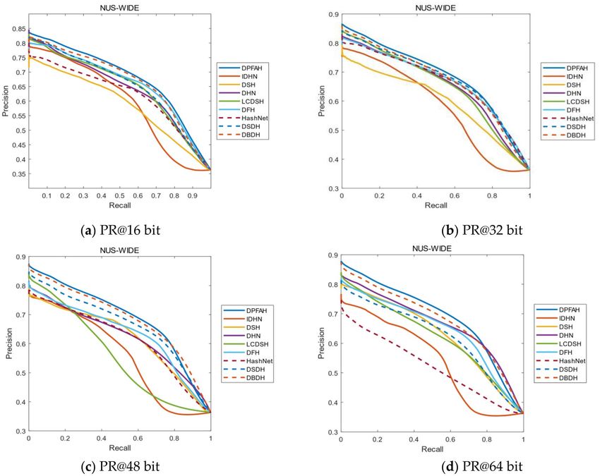
www.nature.com/scientificreports/
PFA module
Channel variance
H H
H X1
X
C C
C
W W W
: Sigmoid : Element-wise multiply
X : Input feature maps X1 : Output feature maps
Figure 2. The detail of PFA module. The mean value of input feature maps X and the channel variance are
computed to judge the importance of each channel and spatial, so as to generate 3-D weights. Then 3-D weights
are processed by the sigmoid activation function and multiplied by X to obtain the output feature maps X1.
(Created by ‘Microsoft Office Visio 2013’ url: https://www.microsoft.com/zh-cn/microsoft-365/previous-versi
ons/microsoft-visio-2013).
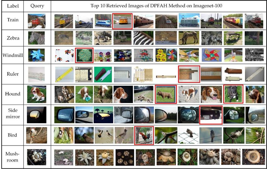
Images
ResNet18
ResNet18+PFA
Dog Zebra Cock Mushroom
Figure 3. Visualization of feature activations. (Created by ‘Microsoft Office Visio 2013’ url: https://www.micro
soft.com/zh-cn/microsoft-365/previous-versions/microsoft-visio-2013).
PFA module. The existing attention modules consider the channel-wise attention or spatial-wise attention
respectively. For channel-wise attention, the importance of each channel is firstly calculated from the perspective
of channels, and then the channel with high importance is assigned greater 1-D weights. For spatial-wise atten-
tion, the importance of features at each location is calculated from a spatial point of view, and then the location
with higher importance is assigned greater 2-D weights. These modules can increase the computational over-
head when computing the 1-D or 2-D attention weights. Hence, this paper introduces a lightweight attention
module (PFA) that can directly calculate 3-D weights. As shown in Fig. 2, first, the mean of X of feature maps X
is obtained and calculate the square of X and X to get the variance. The variance is then divided by the feature
map to obtain the variance of each channel, which is used to determine the variance of each channel and the
importance of each spatial. Finally, the sigmoid function is used to restrict the result, and then multiplied with
the original feature map X . In addition, the PFA module can focus on the primary areas close to the image label.
As shown in Fig. 3, the second line represents the distribution of features extracted using the ResNet18 network,
and the third line represents the PFA module is added to the network. The label of the first image is dog, only
using the ResNet18 network to extract features will pay attention to many noises outside the label. After add-
ing PFA, feature activations are mainly distributed around dog. It has the same effect on the second image. The
third and fourth image focuses on more feature activations information about labels after adding PFA. Hence,
the effectiveness of the PFA module is proved by the visualization of feature activation shown by Grad-CAM39.
Thanks to the PFA introduces an energy function that derives a closed-form solution, it does not add param-
eters to the network. Inspired by neuroscience t heories40, the neurons with the most information are usually the
ones that show different firing patterns from those around them, and then those important neurons should be
Scientific Reports | (2022) 12:7082 | https://doi.org/10.1038/s41598-022-11217-5 4
Vol:.(1234567890)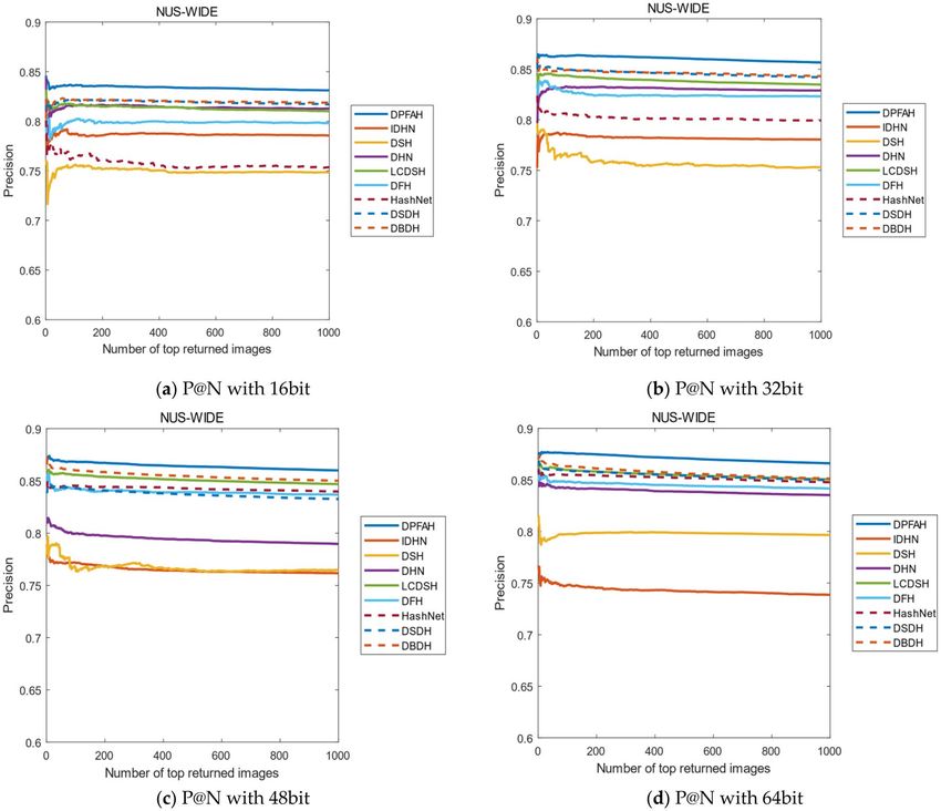
www.nature.com/scientificreports/
given higher priority. The simplest means to discover these neurons is to compute the linear relationship between
one target neuron and the others. Consequently, an energy function for each neuron is defined as follows:
M−1
1
xi )2 (4)
et wt , bt , y, xi = yt −
t + (y0 −
M−1
i=1
where t is target neuron and xi is surrounding neurons in each channel of feature map X ∈ RC×H×W , wt and bt
are weight and bias, i is the ith spatial dimension, M is the number of neurons on a channel and M = H × W ,
t = wt t + bt and xi = wt xi + bt are linear transforms of t and xi . yt and y0 is the output of target neuron and
surrounding neurons respectively and yt = y0. The minimum value is gained by Eq. (4) when yt = t and y0 = xi.
In a channel, the linear separability between target neuron and other neurons can be obtained by calculating the
minimum value of Eq. (4). For simplicity, this paper adopts yt = 1 and y0 = −1, add a regularization term to
optimize the function. The energy function is transformed as follows:
M−1
1
(−1 − (wt xi + bt ))2 + (1 − (wt xi + bt ))2 + wt2 (5)
et wt , bt , y, xi =
M−1
i=1
There are M energy functions on each channel, which are quite complex in calculation by using iterative.
Luckily, Eq. (5) has a fast closed-form solution with respect to wt and bt as follows:
2(t − µt )
wt = − (6)
(t − µt )2 + 2σt2 + 2
1
bt = − (t + µt )wt (7)
2
1 M−1 1 M−1
where µt=M−1 i=1 xi and σt = M−1
2
i=1 (x i − µt ) represents the mean and variance of surrounding neu-
2
rons, respectively. Thanks to the solutions of Eqs. (6) and (7) are calculated on a single channel. This supposes
that all features in a single channel follows the same distribution. The mean and variances of all neurons can
be computed according to this suppose. This method considerably reduces the calculation cost. Therefore, the
minimal energy can be computed as follows:
σ 2 + )
4(
et∗ =
2 (8)
t−µ
+ 2 σ 2 + 2
where µ = M1 M−1 2 = M1 M−1
i=1 xi and σ )2. From Eq. (8), it can be concluded that the greater the dif-
i=1 (x i − µ
ference between the target neuron and the surrounding neurons, the lower the energy function and the more
stable the model will be. Although et∗ can represent the importance of each neuron, this method needs to cal-
culate a large number of covariance matrix. Hence, this paper utilizes a scaling operator instead of an addition
for feature refinement as follows:
1
X̃ = sigmoid ⊙X (9)
E
where E group all et∗ across channel and spatial dimensions. Adding a sigmoid function to prevent the value of
E from being too large.
Model formulation. Input a pair of images xi and xj into the network to generate hash codes bi and bj . The
Hamming distance between bi and bj is defined as DH = 12 (l − �bi , bj �), where bi , bj
is the inner product and l
is the length of hash codes. It can be seen that there are opposite changes between inner product and Hamming
distance. The larger DH , the smaller bi , bj
, and vice versa. Hence, the inner product is used instead of hamming
distance to judge the similarity of pairwise images.
Given the set B = [b1 , b2 , . . . , bn ] of hash codes. The Maximum Likelihood estimation of B for dataset X is
defined as follows:
logP(S|B) = logP(sij |B)
(10)
sij ∈S
where P(S|B) represents the likelihood function. For each image pair, P sij |bi , bj is the conditional probability
of sij under the given premise of bi and bj , which is calculated as follows:
σ �ui , uj � ,
sij = 1
P sij |bi , bj =
1 − σ �ui , uj � , sij = 0
s
1−s
= σ �ui , uj � ij (1 − σ �ui , uj � ) ij (11)
Scientific Reports | (2022) 12:7082 | https://doi.org/10.1038/s41598-022-11217-5 5
Vol.:(0123456789)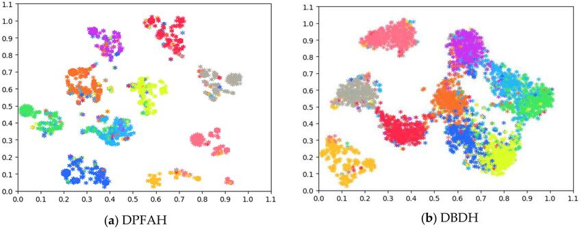
www.nature.com/scientificreports/
where σ (·) is sigmoid function defined as σ (x) = 1+e1 −x and bi = sign(ui ). The reason why this paper uses ui
instead of bi is that bi will cause a discrete optimization problem in Eq. (11). ui is the continuous like-binary codes
output by the network, which can avoid this problem.
Learning hash codes by combing Eqs. (10) and (11) as follows:
L1 = −logP(S|B) = − logP sij |B
sij ∈S
=− (sij �ui , uj � − log(1 + exp(�ui , uj �)))
(12)
sij ∈S
Equation (12) is the negative log likelihood loss function that shows the inner product of similar images
should be as large as possible, the inner product of dissimilar images should be as small as possible. In other
words, the hash codes of similar images are similar, and vice versa. Consequently, the hash codes preserve the
similarity relation of the images in the original space.
In addition, there is an inevitable quantization error when ui is quantized to bi. To solve this problem, inspired
by9, this paper has made the following improvements to ui:
n
L2 = ReLU(−δ − ui ) + ReLU(ui − δ) (13)
i=1
where ReLU(x) = max(0, x) is the Rectified Linear Unit. This paper follows the optimization policy proposed
by34, which relax ui to [−δ, δ] and δ is set to 1.1.
Finally, in the classification layer, the output nodes of the network are determined by c that is the number
of categories in the dataset. The loss between the output of the classification layer and the label yi is defined as:
n
−oi
1
e
L3 = − yi log + 1 − yi log (14)
1 + e−oi 1 + e−oi
i=1
n
{oi − yi oi + log 1 + e−oi }
=−
i=1
Additionally, oi is the real-valued classification layer outputs of the ith image. By calculating Eq. (14), the
generated hash codes by hashing layer saves classification information at the same time.
Overall, combing Eqs. (12), (13) and (14), the total loss of the framework model is expressed as:
Lall = L1 + ηL2 + ζ L3 (15)
Learning. The network parameters are optimized by calculating the gradient of the loss function and com-
pleting the back propagation. To learning a hash function for mapping images to hash codes, θ stands for the
parameters of all feature layers, ϕ(xi ; θ) denotes the output of network, W T ǫR512×l is the transpose of the weight
matrix and v ∈ Rl×1 represents bias vector. A fully connected layer is employed to connect feature representation
and hashing learning. It is set:
ui = W T ϕ(xi ; θ) + v (16)
In the DPFAH model, the parameters to be optimized are θ , W , v and bi . The control variables method is
adopted to optimize the parameters. Among them, bi can be directly optimized:
bi = sign(ui ) (17)
Before optimizing the parameters θ , W and v , this paper calculates the derivative of Lall with respect to ui
and oi by Eq. (15) as:
∂Lall 1 1 ∂L2
= (a − sij )uj + (a − sji )uj + η (18)
∂ui 2 j:s ∈S ij 2 j:s ∈S ji ∂ui
ij ji
where,
n, ui ≥ δ
∂L2
= 0, −δ < ui < δ (19)
∂ui −n, ui ≤ −δ
∂Lall e−oi
= ζ (1 − yi − ) (20)
∂oi 1 + e−oi
Then, this paper updates the parameters W and v by using back propagation:
Scientific Reports | (2022) 12:7082 | https://doi.org/10.1038/s41598-022-11217-5 6
Vol:.(1234567890)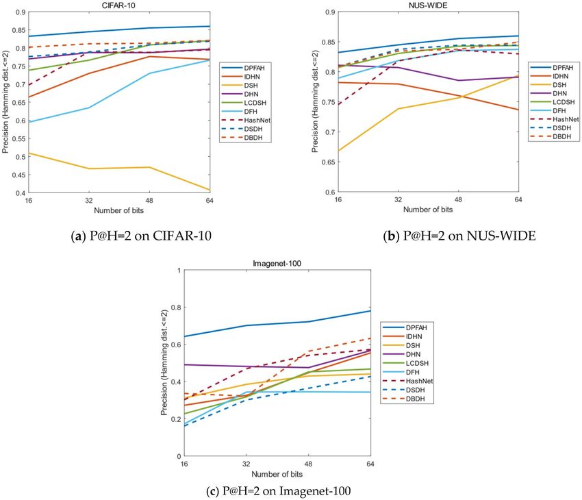
www.nature.com/scientificreports/
Algorithm 1. DPFAH
Input:
Datasets = { } =1 and supervised information constituted of = { } =1 .
Output:
By calculating the partial derivative of each variable, the updated parameters ,
, and .
Initialization:
The parameters of pretrained ResNet18 model and obtained and from
Gaussian distribution.
Repeat:
Randomly choose a batch-size of images from ;
Calculate ( ; ) by forward-propagation;
Calculate = ( ; )+ and = ( );
Calculate the derivatives of , , according to Equation (21), (22) and (23);
Update , , ;
Until:
Traversal completed.
∂Lall ∂Lall T
= ϕ(xi ; θ)( ) (21)
∂W ∂ui
∂Lall ∂Lall
= (22)
∂v ∂ui
When optimizing network parameters, l3 has a certain impact on parameter during back propagation, accord-
ing to Eqs. (18) and (20), the gradient of θ is calculated as:
∂Lall ∂Lall ∂Lall
=W + (23)
∂ϕ(xi ; θ) ∂ui ∂oi
The training process of the DPFAH model is exhibited in Algorithm 1.
Experiments
In this section, the DPFAH model is measured on three datasets. This paper compares the evaluation indexes of
the DPFAH with the latest approaches.
Datasets. (1) CIFAR-10 is a single-label public dataset, which include 60,000 images belonging to 10 classes,
and each class have 6000 images. In this experiment, the training set is composed by selecting 500 images at
random in each class, the testing set is formed by 100 images in each class. The remaining images are treated as
the database. (2) NUS-WIDE is a multi-label public dataset including 269,648 images, this experiment selects
195,834 images belonging to 21 categories from them. Specifically, 100 images from each category form the test-
ing set and the rest of images serve as the dataset. This experiments randomly select 500 images in each class
as training set from the dataset. (3) Imagenet-100 is a single-label public dataset with 138,503 images and each
image belongs to one of 100 classes. In experiment, the testing set is formed by 5000 randomly selected images,
and the rest of the images serve as the database. At the same time, 130 images from each class of the dataset are
chose as training set. In addition, the above three datasets are open-source datasets. All the procedures were
performed in accordance with the relevant guidelines and regulations.
Evaluation metrics and settings. There are four evaluation metrics in the experiment to measure the
performance of DPFAH: mean average precision (mAP), precision-recall curves (PR), precision curves within
Hamming distance 2 (P@H = 2) and precision curves of the first 1000 retrieval results (P@N). In addition, this
paper selects mAP@ALL for CIFAR-10, mAP@5000 for NUS-WIDE and mAP@1000 for Imagenet-100. In order
to prove the performance of DPFAH, the methods of DBDH14, DSDH5, DHN4, LCDSH6, HashNet18, IDHN7,
DFH13 and D SH3 are selected for comparative experiment.
Scientific Reports | (2022) 12:7082 | https://doi.org/10.1038/s41598-022-11217-5 7
Vol.:(0123456789)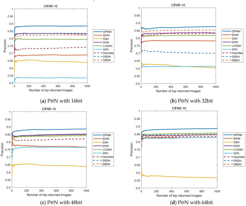
www.nature.com/scientificreports/

                                            Layer                Configuretion
                                            Conv1                {64 × 112 × 112, k = 7 × 7, s = 2 × 2, p = 3 × 3, ReLU}
                                            Maxpool              {64 × 54 × 54, k = 3 × 3, s = 2 × 2, p = 1 × 1, ReLU}
                                            Layer1               {64 × 56 × 56, k = 3 × 3, s = 1 × 1, p = 1 × 1, ReLU} × 4
                                            Layer2               {128 × 28 × 28, k = 3 × 3, s = 2 × 2, p = 1 × 1, ReLU} × 4
                                            Layer3               {256 × 14 × 14, k = 3 × 3, s = 2 × 2, p = 1 × 1, ReLU} × 4
                                            Layer4               {512 × 7 × 7, k = 3 × 3, s = 2 × 2, p = 1 × 1, ReLU} × 4
                                            Avgpool              512 × 1 × 1
                                            Hashing Layer        l , the length of hash codes

                                           Table 1.  Configuration of ResNet18 network.

                                            Item       Configuration
                                            OS         Ubuntu 16.04(× 64)
                                            GPU        Tesla V100

                                           Table 2.  Environment configuration.

                                                      CIFAR-10 (mAP@ALL)                         NUS-WIDE (mAP@5000)
                                            ζ         16 bit    32 bit     48 bit    64 bit      16 bit    32 bit    48 bit    64 bit
                                            0.05      0.7929    0.8161     0.8445    0.8264      0.8246    0.8442    0.8506    0.8538
                                            0.1       0.8382    0.8445     0.8522    0.8549      0.8288    0.8490    0.8541    0.8580
                                            0.5       0.8128    0.8123     0.8293    0.8444      0.8104    0.8407    0.8516    0.8534
                                            1.0       0.8077    0.8285     0.8208    0.8363      0.8013    0.8342    0.8406    0.8436

                                           Table 3.  mAP for of different ζ.

                                                     CIFAR-10 (mAP@ALL)                         NUS-WIDE (mAP@5000)
                                            η        16 bit    32 bit     48 bit    64 bit      16 bit    32 bit    48 bit    64 bit
                                            1        0.8134    0.8331     0.8345    0.8338      0.8238    0.8456    0.8517    0.8550
                                            5        0.8237    0.8168     0.8239    0.8395      0.8232    0.8475    0.8547    0.8593
                                            10       0.8382    0.8445     0.8522    0.8549      0.8288    0.8490    0.8541    0.8580
                                            15       0.8153    0.8173     0.8377    0.8391      0.8160    0.8430    0.8512    0.8541

                                           Table 4.  mAP for of different η.

                                               To make the experimental results objective and impartial, all comparative experiments are carried out on
                                           ResNet18 network and the Pytorch framework. Moreover, the parameter information of ResNet18 in each layer
                                           is shown in Table 1. Specifically, p is the size of the convolution kernel, s and k represent the stride and padding,
                                           respectively, and l is the length of hash codes.
                                               In experiment, all comparative approaches use the same training set and testing set. The optimizer uses the
                                           root mean square prop (RMSProp), the mini batch size is set as 128, the learning rate is set as 5 × 10⁻⁵ and the
                                           weight decay is set as 1 × 10⁻⁵. The environment configuration is shown in Table 2.

                                           Hyperparameter analysis. In Eq. (15), this paper uses two hyperparameters η and ζ to weigh the impact of
                                           classification loss and quantization loss on network optimization. The values of η and ζ are determined by experi-
                                           mental results, as shown in Tables 3 and 4. This paper selects single-label dataset CIFAR-10 and multi-label
                                           dataset NUS-WIDE for parameter adjustment. Experiment fixes η = 10 when adjusting ζ . Similarly, experiment
                                           fixes ζ = 0.1 when adjusting η.
                                               As shown in Table 3, the value of mAP is the largest on the two datasets when ζ = 0.1. The mAP decreases
                                           significantly when ζ = 0.05 on CIFAR-10, and mAP on NUS-WIDE is also decreasing slightly. Compared with
                                           ζ = 0.1, the mAP value of ζ = 0.5 decreased by 2.3% and 0.8% on average respectively on CIFAR-10 and NUS-
                                           WIDE. When ζ = 1, map values decreased by an average of 2.4% and 1.8% on two datasets. Therefore, it is con-
                                           cluded that when the hyperparameter ζ of class-wise loss is 0.1, the experimental result is better.

          Scientific Reports |   (2022) 12:7082 |                        https://doi.org/10.1038/s41598-022-11217-5                                           8

Vol:.(1234567890)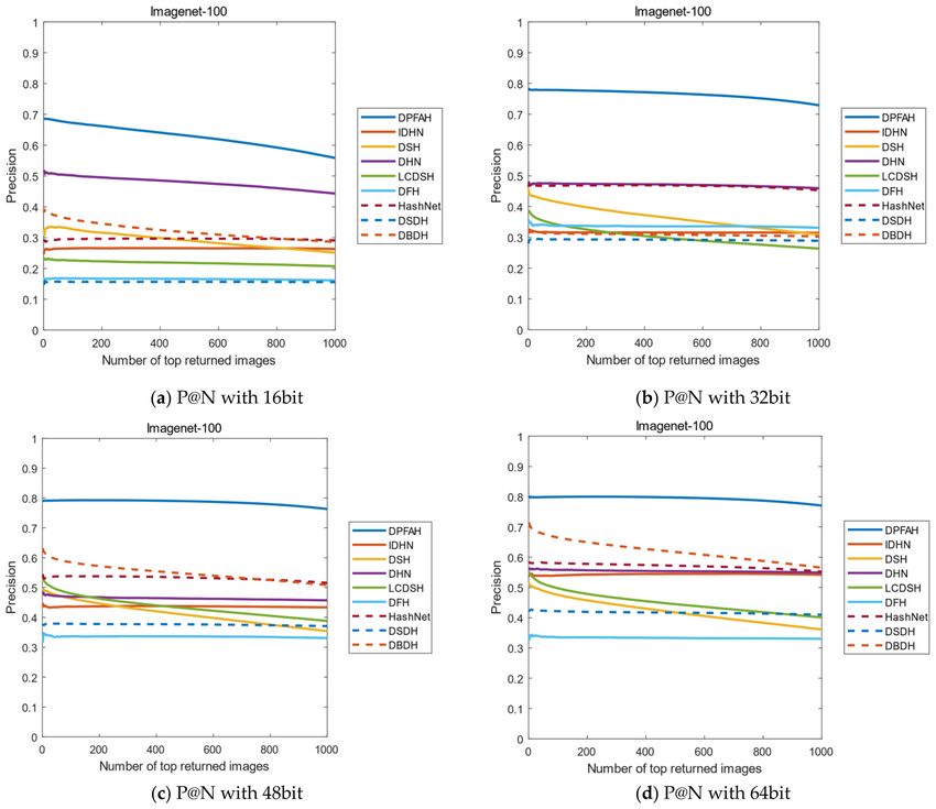
www.nature.com/scientificreports/
Figure 4. (a,b) Represent mAP on different ζ . (Created by “matlab R2019a” url: https://ww2.mathworks.cn/
products/matlab.html).
Figure 5. (a,b) Represent mAP on different ζ . (Created by “matlab R2019a” url: https://ww2.mathworks.cn/
products/matlab.html).
Figure 3 shows mAP on different ζ more intuitively, the mAP curves reach the peak when the value of a is
0.1. As the value of ζ becomes larger or smaller, the value of mAP will decrease slightly. Therefore, this paper
chooses ζ = 0.1 to achieve the optimal experimental effect.
As shown in Table 4, When η = 10, mAP reaches its maximum value. On CIFAR-10 and NUS-WIDE, com-
pared with η = 10, the mAP value of η = 1 decreased by 1.9% and 0.3% on average, the mAP value of η = 5
decreased by 2.1% and 0.1% on average, and the mAP value of η = 15 decreased by 2.0% and 0.6% on average
respectively. Therefore, when the hyperparameter η of quantization loss is 10, good results can be obtained in
the experiment.
Similarly, as shown in Fig. 5, the value of mAP is higher than the others when η = 10, and the mAP curves
reach the peak on CIFAR-10. On NUS-WIDE, when η takes 5 and 10, the mAP at 48 bit and 64 bit are close, but
the mAP value of η = 10 is significantly better than η = 5 at 16 bit and 32 bit. Therefore, this paper also sets η as
10 to achieve optimal experimental effect.
Empirical analysis. In order to fully extract image features without increasing network complexity, this
paper adds the PFA module to ResNet18 network, which can extract 3-D weights of features. Compared with
the common attention mechanism module, the structure of PFA is simple and parameters-free. Meanwhile,
to improve the discrimination and accuracy of hash codes, this paper designs classification branches in the
network. Equation (13) is designed to reduce quantization errors. Equation (14) is the class-wise loss generated
by the classification layer. Equations (13) and (14) are integrated to Lloss in ablation experiments. As shown in
Table 5, DBDH is selected as the baseline and the length of hash codes is 48 bit on CFIAR-10 dataset. DBDH
indicates the baseline model utilizing AlexNet network. DFPAH-1 chooses ResNet18 as backbone instead of
Scientific Reports | (2022) 12:7082 | https://doi.org/10.1038/s41598-022-11217-5 9
Vol.:(0123456789)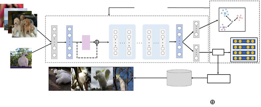
www.nature.com/scientificreports/
Modules DBDH DFPAH-1 DFPAH-2 DFPAH-3
Alexnet √
ResNet18 √ √ √
PFA Module √ √
Lloss √
mAP(48bit) 0.7839 0.8129 0.8424 0.8522
Table 5. Ablation experiments.
Figure 6. (a,b) Present the PR curves and P@N curves, respectively. (Created by “matlab R2019a” url: https://
ww2.mathworks.cn/products/matlab.html).
AlexNet. On this basis, DFPAH-2 shows that PFA Module has been added to the network. DFPAH-3 adds Lloss
to the network. The symbol √ indicates adding corresponding module.
As shown in Table 5, PFA module is added on the basis of DFPAH-1, and the mAP value is increased by
2.95%, which proves that PFA module improves the accuracy of image retrieval. The mAP value of DFPAH-3 is
up to 0.98% higher than DFPAH-2, showing the effectiveness of Lloss.
Figure 6a intuitively shows the PR curves added with PFA module and Lloss , which is significantly higher
than the baseline model. Figure 6b displays the precision of returning the first 1000 images, DFPAH-3 is obvi-
ously better than others. Hence, the above ablation experiments verify the effectiveness of PFA module and Lloss.
Visualization of hash codes by t‑SNE. Figure 7 shows the t-SNE Visualization of the hash codes learned
by DPFAH and the baseline DBDH on CIFAR-10 dataset. As shown in Fig. 7a, the hash codes generated by
DPFAH show clear discriminative structures where the hash codes in different categories are well separated,
while the hash codes generated by DBDH do not show such clear structures. This verifies that by introducing
the PFA module and Lloss for hashing, the hash codes generated through DPFAH are more discriminative than
that generated by DBDH. Therefore, DPFAH method effectively increases the spacing between inter classes and
reduces the gap intra classes, making the generated hash codes compact and effectively enhancing the represen-
tation ability.
Results analysis. As shown in Table 6, it shows the mAP results of all comparative experiments on the
CIFAR-10, NUS-WIDE and Imagenet-100. Experiments select the length of hash codes from 16 to 64 bit. The
mAP of DPFAH have reached 83.82%, 84.45%, 85.22% and 85.49% on the CIFAR-10, which improved by an
average of 3.57% compared to the baseline model. On the NUS-WIDE dataset, the mAP of DPFAH in differ-
ent hash codes length achieves 82.98%, 84.90%, 85.41% and 85.80%. Compared with the classic methods DHN
on the CIFAR-10, DPFAH have improved by 6.87%, 5.74%, 6.53% and 5.83% respectively. On the NUS-WIDE
dataset, DPFAH achieves 1.90%, 4.21%, 6.87% and 6.70% growth compared with DHN on different bits. On the
Imagenet-100 dataset, the effect of DPFAH is the most obvious in three datasets, compared with baseline model
DBDH, DPFAH has achieves 30.62%, 37.94%, 15.86% and 14.74% on different bits. Hence, a large number of
experiments show that the model trained by DPFAH has higher robustness.
The curve of PR is an evaluation index with precision and recall as variables. Recall in the curve is set as the
abscissa and precision is set as the ordinate. If the PR curve of one algorithm is completely surrounded by another
algorithm, it can be asserted that the performance of the latter is better than that of the former. Therefore, the
performance of the algorithm is judged by the area enclosed by the PR curve. Figure 8 shows the PR curves on
Scientific Reports | (2022) 12:7082 | https://doi.org/10.1038/s41598-022-11217-5 10
Vol:.(1234567890)www.nature.com/scientificreports/
Figure 7. (a,b) Present the t-SNE visualization of hash codes on CIFAR-10. (Created by “python3.6” https://
www.python.org/downloads/release/python-3614).
CIFAR-10 (mAP@ALL) NUS-WIDE (mAP@5000) Imagenet-100 (mAP@1000)
Method 16bit 32bit 48bit 64bit 16bit 32bit 48bit 64bit 16bit 32bit 48bit 64bit
DPFAH 0.8382 0.8445 0.8522 0.8549 0.8298 0.8490 0.8541 0.8580 0.6420 0.7009 0.7212 0.7795
DBDH 0.8021 0.8113 0.8129 0.8209 0.8084 0.8345 0.8393 0.8492 0.3358 0.3215 0.5626 0.6321
DSDH 0.7761 0.7881 0.8086 0.8183 0.8085 0.8373 0.8265 0.8441 0.1612 0.3011 0.3638 0.4268
DHN 0.7695 0.7871 0.7869 0.7966 0.8108 0.8069 0.7854 0.7910 0.4900 0.4808 0.4747 0.5664
LCDSH 0.7383 0.7661 0.8083 0.8202 0.8071 0.8304 0.8425 0.8436 0.2269 0.3177 0.4517 0.4671
Hashnet 0.6975 0.7892 0.7878 0.7949 0.7453 0.8004 0.8268 0.8297 0.3017 0.4690 0.5400 0.5719
IDHN 0.6641 0.7296 0.7762 0.7681 0.7820 0.7795 0.7601 0.7366 0.2721 0.3255 0.4477 0.5539
DFH 0.5947 0.6347 0.7298 0.7662 0.7893 0.8185 0.8350 0.8372 0.1727 0.3435 0.3445 0.3430
DSH 0.5095 0.4663 0.4702 0.4714 0.6680 0.7383 0.7563 0.7940 0.3109 0.3848 0.4294 0.4403
Table 6. mAP for different bit on three datasets. Significant values are in bold.
dataset CIFAR-10. As can be seen from the Figure 8a–d, the curves of DPFAH method are significantly higher
than all comparative methods. In particular, when the length of hash codes is 16bit, the enclosed area is much
larger than DSDH, which has the best performance among all comparative methods.
Because NUS-WIDE is a multi-label dataset and the calculation process is relatively complex, the improve-
ment on NUS-WIDE is not as obvious as that on CIFAR-10, but it is still the best of all methods. As shown in Fig-
ure 9, the mAP of DPFAH is the highest compared with the other eight comparison algorithms. In Figure 9a–d,
DPFAH is higher than DSDH that has the best performance among all methods.
Figure 10 shows the PR curves of 16, 32, 48 and 64 bits on Imagenet-100 dataset. The PR curve of DPFAH
method is significantly higher than that of other comparison methods, especially on Fig. 10b–d In Fig. 10a, when
recall is greater than about 0.6, the precision of DPFAH is less than that of DHN. When recall is less than 0.6,
the precision of DPFAH is much higher than that of DHN. It can be seen from the overall PR curve siege area
that DPFAH is significantly greater than DHN.
To achieve the aim that the hamming ranking only needs O(1) time searches, the evaluating indicator P@H = 2
is important for the retrieval of hash codes. Figure 11 shows the result of P@H = 2 on three datasets, the method
DPFAH obtains the highest precision in experiment. With the increase of hash code length, the precision also
increases steadily, which shows that DPFAH model is more stable than the methods of DSH, IDHN and DHN
on CIFAR-10, NUS-WIDE and Imagenet-100.
Another evaluation metric is the curves of P@N. The precision of the first 1000 images are selected in this
experiment. Figure 12 shows the result of P@N on CIFAR-10 dataset, DPFAH method has achieved better preci-
sion than the other methods. Specifically, in Fig. 12a, the curves P@N of DPFAH is significantly higher than DHN
and DSDH. In Fig. 12b–d, although the growth rate of DPFAH is not as obvious as Fig. 12a, the best precision
is still obtained on 32bit, 48bit and 64bit.
Scientific Reports | (2022) 12:7082 | https://doi.org/10.1038/s41598-022-11217-5 11
Vol.:(0123456789)www.nature.com/scientificreports/
Figure 8. (a–d) The PR curves on CIFAR-10 of all methods with different bits. (Created by “matlab R2019a”
url: https://ww2.mathworks.cn/products/matlab.html).
Figure 13 shows the P@N curves on NUS-WIDE, as can be from Fig. 13a,b, the P@N curves of all methods
is relatively stable with the number of returned images increases. Compared with other algorithms, DPFAH still
achieves the highest precision.
Figure 14 shows the P@N curves on the Imagenet-100 dataset. As can be seen from Figure 14b–d, when the
length of the hash codes is 32, 48 and 64bits, the effect of DPFAH is obviously better than the other methods. With
the increase of the number of images, the precision shows a stable trend, but the best results are still obtained
in all comparison algorithms.
Visualization show. In Fig. 15, this paper visualizes the top 10 returned images of DPFAH for eight query
images on Imagenet-100. The first row shows the label of the query images, the second row is query images, the
retrieval results of DPFAH are shown at other rows. The red boxes are used to mark the false retrieval results.
Conclusions
Existing image retrieval methods based on deep hashing have the defects of imbalance and insufficiency when
existing hashing methods extract image features. Some scholars propose to employ channel-wise or spatial-wise
attention mechanism into the network, which will add many parameters to the model and increase the computa-
tional complexity. Hence, this paper introduces a PFA module and propose DPFAH method. PFA module based
on well-established suppression theory and define an energy function that determine the importance of each
neuron. This module does not add any parameters to the network and directly extracts 3-D weight information
of feature map. In addition, to generate accurate hash codes that retain the similarity information of the original
image, this paper designs a classification branch to optimal network. The effectiveness of DPFAH method is
proved by a large number of experiments. In particular, the evaluation index mAP increased by 2.95% when the
PFA module is added in network. Hence, a better image retrieval model is obtained by DPFAH method.
Scientific Reports | (2022) 12:7082 | https://doi.org/10.1038/s41598-022-11217-5 12
Vol:.(1234567890)www.nature.com/scientificreports/
Figure 9. (a–d) Represent the PR curves on NUS-WIDE of all methods with different bits. (Created by “matlab
R2019a” url: https://ww2.mathworks.cn/products/matlab.html).
Scientific Reports | (2022) 12:7082 | https://doi.org/10.1038/s41598-022-11217-5 13
Vol.:(0123456789)www.nature.com/scientificreports/
(a) PR@16 bit (b) PR@32 bit
(c) PR@48 bit (d) PR@64 bit
Figure 10. (a–d) Represent the PR curves on Imagenet-100 of all methods with different bits. (Created by
“matlab R2019a” url: https://ww2.mathworks.cn/products/matlab.html).
Scientific Reports | (2022) 12:7082 | https://doi.org/10.1038/s41598-022-11217-5 14
Vol:.(1234567890)www.nature.com/scientificreports/
Figure 11. (a–c) Present P@H = 2 on three datasets. (Created by “matlab R2019a” url: https://ww2.mathworks.
cn/products/matlab.html).
Scientific Reports | (2022) 12:7082 | https://doi.org/10.1038/s41598-022-11217-5 15
Vol.:(0123456789)www.nature.com/scientificreports/
Figure 12. (a–d) Represent the P@N curves on CIFAR-10 of all methods with different bit. (Created by “matlab
R2019a” url: https://ww2.mathworks.cn/products/matlab.html).
Scientific Reports | (2022) 12:7082 | https://doi.org/10.1038/s41598-022-11217-5 16
Vol:.(1234567890)www.nature.com/scientificreports/
Figure 13. (a–d) Represent the P@N curves on NUS-WIDE of all methods with different bits. (Created by
“matlab R2019a” url: https://ww2.mathworks.cn/products/matlab.html).
Scientific Reports | (2022) 12:7082 | https://doi.org/10.1038/s41598-022-11217-5 17
Vol.:(0123456789)www.nature.com/scientificreports/
Figure 14. (a–d) Represent the P@N curves on Imagenet-100 of all methods with different bits. (Created by
“matlab R2019a” url: https://ww2.mathworks.cn/products/matlab.html).
Scientific Reports | (2022) 12:7082 | https://doi.org/10.1038/s41598-022-11217-5 18
Vol:.(1234567890)www.nature.com/scientificreports/
Figure 15. Top 10 retrieved results from Imagenet-100 dataset by DPFAH with 64bit hash codes. (Created by
‘Microsoft Office Visio 2013’ url: https://www.microsoft.com/zh-cn/microsoft-365/previous-versions/microsoft-
visio-2013).
Data availability
The CIFAR-10, NUS-WIDE and Imagenet-100 datasets are openly available at: http://www.cs.toronto.edu/kriz/
cifar.h
tml(access ed on 8 April 2022), http://l ms.c omp.n
us.e du.s g/r esear ch/N
US-W
IDE.h
tml (accessed on 8 April
2022) and https://image-net.org (accessed on 8 April 2022).
Received: 23 December 2021; Accepted: 20 April 2022
References
1. Qiao, C., Brown, K., Zhang, F., & Tian, Z.H. Federated adaptive asynchronous clustering algorithm for wireless mesh networks.
in IEEE Transactions on Knowledge and Data Engineering. 3119550. (2021).
2. Lu, H. et al. DeepAutoD: Research on distributed machine learning oriented scalable mobile communication security unpacking
system. in IEEE Transactions on Network Science and Engineering. (2021).
3. Liu, H. & Wang, R. Deep supervised hashing for fast image retrieval. in Proceedings of the IEEE Conference on Computer Vision
and Pattern Recognition. 2064–2072 (2016).
4. Zhu, H. et al. Deep hashing network for efficient similarity retrieval. Proc. AAAI Conf. Artif. Intell. 30, 1 (2016).
5. Jiang, Q. Y., Cui, X. & Li, W. J. Deep supervised discrete hashing. IEEE Trans. Image Process. 27, 5996–6009 (2018).
6. Zhu, H., Gao, S. Locality constrained deep supervised hashing for image retrieval. in Proceedings of the International Conference
on Artificial Intelligence. 3567–3573. (2017).
7. Zhang, Z. et al. Improved deep hashing with soft pairwise similarity for multi-label image retrieval. IEEE Trans. Multimed. 22,
540–553 (2019).
8. Yan, X., Zhu, F. & Yu, P. S. Feature-based similarity search in graph structures. ACM Trans. Database Syst. 31, 1418–1453 (2006).
9. Cheng, H.D. & Shi, X.J. A simple and effective histogram equalization approach to image enhancement. Digital Signal Process.
158–170. (2004).
10. Liu, D., Shen, J., Xia, Z. & Sun, X. A content-based image retrieval scheme using an encrypted difference histogram in cloud
computing. Information 8, 96 (2017).
11. Zheng, L. & Yang, Y. A decade survey of instance retrieval. IEEE Trans. Pattern Anal. Mach. Intell. 40, 1224–1244 (2018).
12. Cheng, S., Wang, L. & Du, A. Deep semantic-preserving reconstruction hashing for unsupervised cross-modal retrieval. Entropy
22, 1266 (2020).
13. Li, Y. & Pei, W. Push for Quantization: Deep Fisher Hashing. arXiv preprint arXiv:1909.00206 (2019).
14. Zheng, X., Zhang, Y. & Lu, X. Q. Deep balanced discrete hashing for image retrieval. Neurocomputing 403, 224–236 (2020).
15. Paulevé, L., Jégou, H. & Amsaleg, L. Locality sensitive hashing: A comparison of hash function types and querying mechanisms.
Pattern Recognit. Lett. 31, 1348–1358 (2010).
16. Bai, X. et al. Data-dependent hashing based on p-stable distribution. IEEE Trans. Image Process. 23, 5033–5046 (2014).
Scientific Reports | (2022) 12:7082 | https://doi.org/10.1038/s41598-022-11217-5 19
Vol.:(0123456789)www.nature.com/scientificreports/
17. Lv, N. & Wang, Y. Deep hashing for motion capture data retrieval. in Proceedings of the IEEE International Conference on Acoustics,
Speech and Signal Processing (ICASSP). 2215–2219. (2021).
18. Cao, Z. et al. HashNet: Deep learning to hash by continuation. in Proceedings of the IEEE International Conference on Computer
Vision. 5608–5617. (2017).
19. Li, X. et al. Image retrieval using a deep attention-based hash. IEEE Access. 8, 142229–142242 (2020).
20. Yang, L., Zhang, R.Y., Li, L. & Xie, X.H. Simam: A simple, parameter-free attention module for convolutional neural networks.
in International Conference on Machine Learning. 11863–11874. (2021).
21. Zhe, X. et al. Semantic Hierarchy Preserving Deep Hashing for Large-Scale Image Retrieval. arXiv:1901.11259 (2019).
22. Chai, Y.H. et al. Dynamic prototype network based on sample adaptation for few-shot malware detection. in IEEE Transactions
on Knowledge and Data Engineering. (2022).
23. Luo, C. C. et al. A novel web attack detection system for internet of things via ensemble classification. IEEE Trans. Indus. Inf. 17,
5810–5818 (2020).
24. Sun, Y. et al. Honeypot identification in softwarized industrial cyber-physical systems. IEEE Trans. Indus. Inf. 17, 5542–5551 (2021).
25. Qiu, J. et al. Nei-TTE: Intelligent traffic time estimation based on fine-grained time derivation of road segments for smart city.
IEEE Trans. Indus. Inf. 16, 2659–2666 (2020).
26. Weiss, Y. & Torralba, A. Spectral hashing. NIPS 1, 4 (2008).
27. Liu, W. et al. Hashing with graphs. in Proceedings of the 28th International Conference on Machine Learning. (2011).
28. Jin, S., Yao, H. & Sun, X. Unsupervised semantic deep hashing. Neurocomputing 351, 19–25 (2019).
29. Yang, E. et al. Semantic structure-based unsupervised deep hashing. in Proceedings of the 27th International Joint Conference on
Artificial Intelligence. 1064–1070. (2018).
30. Jiang, S., Wang, L. & Cheng, S. Unsupervised hashing with gradient attention. Symmetry. 12, 1193 (2020).
31. Huang, L.K., Chen, J. & Pan, S.J. Accelerate learning of deep hashing with gradient attention. in Proceedings of the IEEE/CVF
International Conference on Computer Vision. 5271–5280. (2019).
32. Xia, R. & Pan, Y. Supervised hashing for image retrieval via image representation learning. in Proceedings of the AAAI Conference
on Artificial Intelligence. Vol. 28. (2014).
33. Li, W.J. & Wang, S. Feature Learning Based Deep Supervised Hashing with Pairwise Labels. arXiv:1511.03855 (2015).
34. Yang, W. et al. Deep hash with improved dual attention for image retrieval. Information 12, 285 (2021).
35. Su, S., Zhang, C., Han, K. & Tian, Y.H. Greedy hash: Towards fast optimization for accurate hash coding in CNN. in Proceedings
of the 32nd International Conference on Neural Information Processing Systems. 806–815. (2018).
36. Zhang, Z., Zou, Q. & Wang, Q. Instance Similarity Deep Hashing for Multi-Label Image Retrieval. arXiv:1803.02987 (2018).
37. Cao, Y. et al. Deep Cauchy hashing for hamming space retrieval. in Proceedings of the IEEE Conference on Computer Vision and
Pattern Recognition. 1229–1237. (2018).
38. Zhe, X., Chen, S. & Yan, H. Deep class-wise hashing: Semantics-preserving hashing via class-wise loss. IEEE Trans. Neural Netw.
Learn. Syst. 31, 1681–1692 (2019).
39. Selvaraju, R., Cogswell, M. & Das, A. Grad-CAM: Visual explanations from deep network via gradient-based localization. in IEEE
Conference on Computer Vision and Pattern Recognition. 618–626. (2017).
40. Webb, B. S., Dhruv, N. T. & Solomon, S. G. Early and late mechanisms of surround suppression in striate cortex of macaque.
Neuroscience 25, 11666–11675 (2005).
Author contributions
Conceptualization, W.Y.; methodology, W.Y.; software, W.Y. and S.C.; validation, S.C. and L.W; formal analysis,
L.W. and S.C.; data curation, W.Y.; writing original draft preparation, W.Y.; writing-review and editing, L.W. and
S.C. All authors have read and agreed to the published version of the manuscript.
Funding
This research was funded by the Tianshan Innovation Team of Xinjiang Uygur Autonomous Region under Grant
2020D14044.
Competing interests
The authors declare no competing interests.
Additional information
Correspondence and requests for materials should be addressed to L.W.
Reprints and permissions information is available at www.nature.com/reprints.
Publisher’s note Springer Nature remains neutral with regard to jurisdictional claims in published maps and
institutional affiliations.
Open Access This article is licensed under a Creative Commons Attribution 4.0 International
License, which permits use, sharing, adaptation, distribution and reproduction in any medium or
format, as long as you give appropriate credit to the original author(s) and the source, provide a link to the
Creative Commons licence, and indicate if changes were made. The images or other third party material in this
article are included in the article’s Creative Commons licence, unless indicated otherwise in a credit line to the
material. If material is not included in the article’s Creative Commons licence and your intended use is not
permitted by statutory regulation or exceeds the permitted use, you will need to obtain permission directly from
the copyright holder. To view a copy of this licence, visit http://creativecommons.org/licenses/by/4.0/.
© The Author(s) 2022
Scientific Reports | (2022) 12:7082 | https://doi.org/10.1038/s41598-022-11217-5 20
Vol:.(1234567890)You can also read