UNSUPERVISED LEARNING OF FULL-WAVEFORM INVERSION: CONNECTING CNN AND PARTIAL DIFFERENTIAL EQUATION IN A LOOP
←
→
Page content transcription
If your browser does not render page correctly, please read the page content below
Under review as a conference paper at ICLR 2022

U NSUPERVISED L EARNING OF F ULL -WAVEFORM
I NVERSION : C ONNECTING CNN AND PARTIAL
D IFFERENTIAL E QUATION IN A L OOP
 Anonymous authors
 Paper under double-blind review

                                           A BSTRACT
         This paper investigates unsupervised learning of Full-Waveform Inversion (FWI),
         which has been widely used in geophysics to estimate subsurface velocity maps
         from seismic data. This problem is mathematically formulated by a second order
         partial differential equation (PDE), but is hard to solve. Moreover, acquiring ve-
         locity map is extremely expensive, making it impractical to scale up a supervised
         approach to train the mapping from seismic data to velocity maps with convolu-
         tional neural networks (CNN).We address these difficulties by integrating PDE
         and CNN in a loop, thus shifting the paradigm to unsupervised learning that only
         requires seismic data. In particular, we use finite difference to approximate the
         forward modeling of PDE as a differentiable operator (from velocity map to seis-
         mic data) and model its inversion by CNN (from seismic data to velocity map).
         Hence, we transform the supervised inversion task into an unsupervised seismic
         data reconstruction task. We also introduce a new large-scale dataset OpenFWI,
         to establish a more challenging benchmark for the community. Experiment results
         show that our model (using seismic data alone) yields comparable accuracy to the
         supervised counterpart (using both seismic data and velocity map). Furthermore,
         it outperforms the supervised model when involving more seismic data.

Figure 1: Schematic illustration of our proposed method, which comprises a CNN to learn an inverse
mapping and a differentiable operator to approximate the forward modeling of PDE.

1   I NTRODUCTION
Geophysical properties (such as velocity, impedance, and density) play an important role in various
subsurface applications including subsurface energy exploration, carbon capture and sequestration,
estimating pathways of subsurface contaminant transport, and earthquake early warning systems
to provide critical alerts. These properties can be obtained via seismic surveys, i.e., receiving re-
flected/refracted seismic waves generated by a controlled source. This paper focuses on recon-
structing subsurface velocity maps from seismic measurements. Mathematically, the velocity map
and seismic measurements are correlated through an acoustic-wave equation (a second-order partial
differential equation) as follows:
                                              1 ∂ 2 p(r, t)
                               ∇2 p(r, t) −                 = s(r, t) ,                           (1)
                                            v(r)2 ∂t2

                                                 1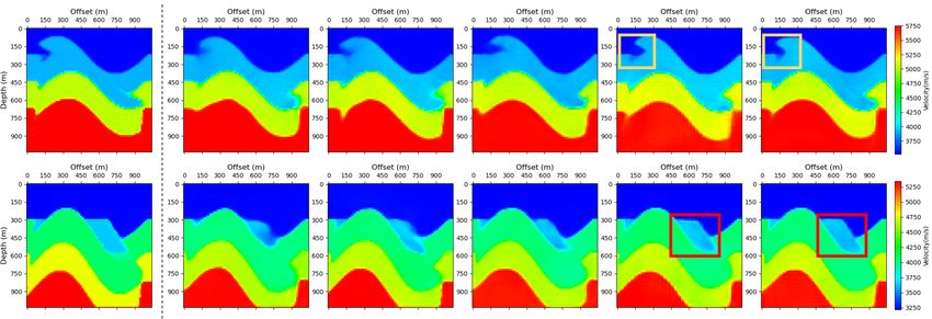
Under review as a conference paper at ICLR 2022

                   (a)                                                 (b)
Figure 2: An example of (a) a velocity map and (b) seismic measurements (named shot gather in
geophysics) and the 1D time-series signal recorded by a receiver.

where p(r, t) denotes the pressure wavefield at spatial location r and time t, v(r) represents the
velocity map of wave propagation, and s(r, t) is the source term. Full Waveform Inversion (FWI) is
a methodology that determines high-resolution velocity maps v(r) of the subsurface via matching
synthetic seismic waveforms to raw recorded seismic data p(r̃, t), where r̃ represents the locations
of the seismic receivers.
A velocity map describes the wave propagation speed in the subsurface region of interest. An exam-
ple in 2D scenario is shown in Figure 2a. Particularly, the x-axis represents the horizontal offset of a
region, and the y-axis stands for the depth. The regions with the same geologic information (veloc-
ity) are called a layer in velocity maps. In a sample of seismic measurements (termed a shot gather
in geophysics) as depicted in Figure 2b, each grid in the x-axis represents a receiver, and the value
in the y-axis is a 1D time-series signal recorded by each receiver.
Existing approaches solve FWI in two directions: physics-driven and data-driven. Physics-driven
approaches rely on the forward modeling of Equation 1, which simulates seismic data from velocity
map by finite difference. They optimize velocity map per seismic sample, by iteratively updating
velocity map from an initial guess such that simulated seismic data (after forward modeling) is close
to the input seismic measurements. However, these methods are slow and difficult to scale up as the
iterative optimization is required per input sample. Data-driven approaches consider FWI problem
as an image-to-image translation task and apply convolution neural networks (CNN) to learn the
mapping from seismic data to velocity maps (Wu & Lin, 2019). The limitation of these methods
is that they require paired seismic data and velocity maps to train the network. Such ground truth
velocity maps are hardly accessible in real-world scenario because generating them is extremely
time-consuming even for domain experts.
In this work, we leverage advantages of both directions (physics + data driven) and shift the paradigm
to unsupervised learning of FWI by connecting forward modeling and CNN in a loop. Specifically,
as shown in Figure 1, a CNN is trained to predict a velocity map from seismic data, which is followed
by forward modeling to reconstruct seismic data. The loop is closed by applying reconstruction loss
on seismic data to train the CNN. Due to the differentiable forward modeling, the whole loop can
be trained end-to-end. Note that the CNN is trained in an unsupervised manner, as the ground
truth of velocity map is not needed. We name our unsupervised approach as UPFWI (Unsupervised
Physical-informed Full Waveform Inversion).
Additionally, we find that perceptual loss (Johnson et al., 2016) is crucial to improve the overall
quality of predicted velocity maps due to its superior capability in preserving the coherence of the
reconstructed waveforms comparing with other losses like Mean Squared Error (MSE) and Mean
Absolute Error (MAE).
To encourage fair comparison on a large dataset with more complicate geological structures, we
introduce a new dataset named OpenFWI, which contains 60,000 labeled data (velocity map and
seismic data pairs) and 48,000 unlabeled data (seismic data alone). 30,000 of those velocity maps
contain curved layers that are more challenge for inversion. We also add geological faults with
various shift distances and tilting angles to all velocity maps.
We evaluate our method on this large dataset. Experimental results show that for velocity maps
with flat layers, our UPFWI trained with 48,000 unlabeled data achieves 1146.09 in MSE, which
is 26.77% smaller than that of the supervised method, and 0.9895 in Structured Similarity (SSIM),

                                                   2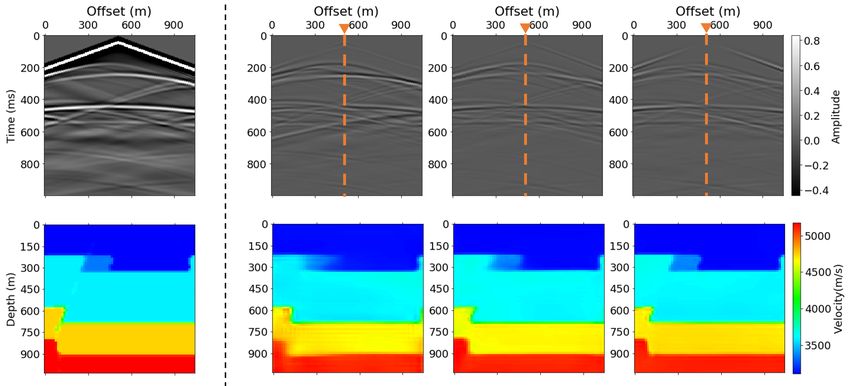
Under review as a conference paper at ICLR 2022

                  Mean Squared Error (MSE)                    Structural Similarity (SSIM)

Figure 3: Unsupervised UPFWI (ours) vs. Supervised H-PGNN+ (Sun et al., 2021). Our method
achieves better performance, e.g. lower Mean Squared Error (MSE) and higher Structural Similar-
ity (SSIM), when involving more unlabeled data (>24k).

which is 0.0021 higher than the score of the supervised method; for velocity maps with curved layers,
our UPFWI achieves 3639.96 in MSE, which is 28.30% smaller than that of supervised method, and
0.9756 in SSIM, which is 0.0057 higher than the score of the supervised method.
Our contribution is summarized as follows:

       • We propose to solve FWI in an unsupervised manner by connecting CNN and forward
         modeling in a loop, enabling end-to-end learning from seismic data alone.
       • We find that perceptual loss is helpful to boost the performance comparable to the super-
         vised counterpart.
       • We introduce a large-scale dataset as benchmark to encourage further research on FWI.

2   P RELIMINARIES OF F ULL WAVEFORM I NVERSION (FWI)
The goal of FWI in geophysics is to invert for a velocity map v ∈ RW ×H from seismic measure-
ments p ∈ RS×T ×R , where W and H denote the horizontal and vertical dimensions of the velocity
map, S is the number of sources that are used to generate waves during data acquisition process,
T denotes the number of samples in the wavefields recorded by each receiver, and R represents the
total number of receivers.
In conventional physics-driven methods, forward modeling is commonly referred to the process
of simulating seismic data p̃ from given estimated velocity maps v̂. For simplicity, the forward
acoustic-wave operator f can be expressed as
                                             p̃ = f (v̂) .                                         (2)

Given this forward operator f , the physics-driven FWI can be posed as a minimization prob-
lem (Virieux & Operto, 2009)
                                        n                       o
                           E(v̂) = min ||p − f (v̂)||22 + λR(v̂) ,                      (3)
                                        v̂

where ||p − f (v̂)||22 is the the `2 distance between true seismic measurements p and the corre-
sponding simulated data f (v̂), λ is a regularization parameter and R(v̂) is the regularization term
which is often the `2 or `1 norm of v̂. This requires optimization per sample, which is slow as the
optimization involves multiple iterations from an initial guess.
Data-driven methods leverage convolutional neural networks to directly learn the inverse mapping
as (Adler et al., 2021)
                                      v̂ = gθ (p) ≈ f −1 (p) ,                                     (4)
where gθ (·) is the approximated inverse operator of f (·) parameterized by θ. In practice, gθ is usu-
ally implemented as a convolutional neural network (Adler et al., 2021; Wu & Lin, 2019). This
requires paired seismic data and velocity maps for supervised learning. However, the acquisition of
large volume of velocity maps in field applications can be extremely challenging and computation-
ally prohibitive.

                                                  3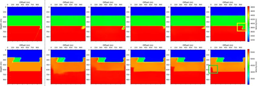
Under review as a conference paper at ICLR 2022

3     M ETHOD
In this section, we present our Unsupervised Physics-informed solution (named UPFWI), which
connects CNN and forward modeling in a loop. It addresses limitations of both physics-driven and
data-driven approaches, as it requires neither optimization at inference (per sample), nor velocity
maps as supervision.

3.1   UPFWI: C ONNECTING CNN AND F ORWARD M ODELING

As depicted in Figure 1, our UPFWI connects a CNN gθ and a differentiable forward operator f
to form a loop. In particular, the CNN takes seismic measurements p as input and generates the
corresponding velocity map v̂. We then apply forward acoustic-wave operator f (see Equation 2)
on the estimated velocity map v̂ to reconstruct the seismic data p̃. Typically, the forward modeling
employs finite difference (FD) to discretize the wave equation (Equation 1). The details of forward
modeling will be discussed in the subsection 3.3. The loop is closed by the reconstruction loss
between input seismic data p and the reconstructed seismic data p̃ = f (gθ (p)). Notice that the
ground truth of velocity maps v is not involved, and the training process is unsupervised. Since
the forward operator is differentiable, the reconstruction loss can be backpropagated (via gradient
descent) to update the parameters θ in the CNN.

3.2   CNN N ETWORK A RCHITECTURE

We use an encoder-decoder structured CNN (similar to Wu & Lin (2019) and Zhang & Lin (2020))
to model the mapping from seismic data p ∈ RS×T ×R to velocity map v ∈ RW ×H . The encoder
compresses the seismic input and then transforms the latent vector to build the velocity estimation
through a decoder. Since the number of receivers R and the number of timesteps T in seismic
measurements are unbalanced (T  R), we first stack a 7×1 and six 3×1 convolutional layers (with
stride 2 every the other layer to reduce dimension) to extract temporal features until the temporal
dimension is close to R. Then, six 3×3 convolutional layers are followed to extract spatial-temporal
features. The resolution is down-sampled every the other layer by using stride 2. Next, the feature
map is flattened and a fully connected layer is applied to generate the latent feature with dimension
512. The decoder first repeats the latent vector by 25 times to generate a 5×5×512 tensor. Then it is
followed by five 3×3 convolutional layers with nearest neighbor upsampling in between, resulting
in a feature map with size 80×80×32. Finally, we center-crop the feature map (70×70) and apply a
3×3 convolution layer to output a single channel velocity map. All the aforementioned convolutional
and upsampling layers are followed by a batch normalization (Ioffe & Szegedy, 2015) and a leaky
ReLU (Nair & Hinton, 2010) as activation function.

3.3   D IFFERENTIABLE F ORWARD M ODELING

We apply the standard finite difference (FD) in the space domain and time domain to discretize
the original wave equation. Specifically, the second-order central finite difference in time do-
        2
main ( ∂ p(r,t)
          ∂t2   in Equation 1) is approximated as follows:
                      ∂ 2 p(r, t)      1
                                  ≈         (pt+1 − 2ptr + pt−1
                                                             r ) + O[(∆t) ] ,
                                                                              2
                                                                                                  (5)
                          ∂t 2       (∆t)2 r
where ptr denotes the pressure wavefields at timestep t, and pt+1  r   and pt−1
                                                                              r are the wavefields at
t + ∆t and t − ∆t, respectively. The Laplacian of p(r, t) can be estimated in the similar way on the
space domain (see Appendix). Therefore, the wave equation can then be written as
                            pt+1
                             r    = (2 − v 2 ∇2 )ptr − pt−1
                                                        r   + v 2 (∆t)2 str ,                     (6)
         2
where ∇ here denotes the discrete Laplace operator.
The initial wavefield at the timestep 0 is set zero (i.e. p0r = 0). Thus, the gradient of loss L with
respect to estimated velocity at spatial location r can be computed using the chain rule as
                                             T
                                   ∂L       X        ∂L      ∂p(r, t)
                                          =                           ,                           (7)
                                  ∂v(r)     t=0
                                                  ∂p(r, t) ∂v(r)
where T indicates the length of the sequence.

                                                 4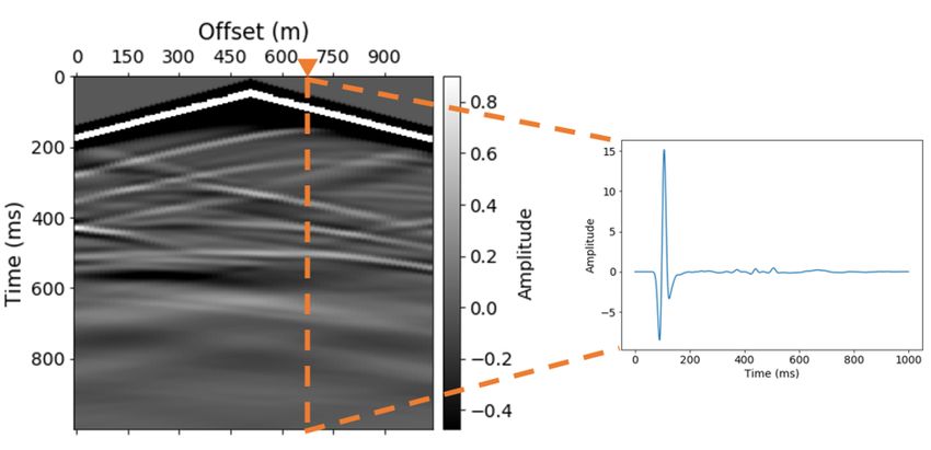
Under review as a conference paper at ICLR 2022

3.4   L OSS F UNCTION

The reconstruction loss of our UPFWI includes a pixel-wise loss and a perceptual loss as follows:
                            L(p, p̃) = Lpixel (p, p̃) + Lperceptual (p, p̃),                       (8)
where p and p̃ are input and reconstructed seismic data, respectively. The pixel-wise loss Lpixel
combines `1 and `2 distance as:
                              Lpixel (p, p̃) = λ1 `1 (p, p̃) + λ2 `2 (p, p̃),                      (9)
where λ1 and λ2 are two hyper-parameters to control the relative importance. For the perceptual
loss Lperceptual , we extract features from conv5 in a VGG-16 network (Simonyan & Zisserman,
2015) pretrained on ImageNet (Krizhevsky et al., 2012) and combine the `1 and `2 distance as:
                    Lperceptual (p, p̃) = λ3 `1 (φ(p), φ(p̃)) + λ4 `2 (φ(p), φ(p̃)),              (10)
where φ(·) represents the output of conv5 in the VGG-16 network, and λ3 and λ4 are two hyper-
parameters. Compared to the pixel-wise loss, the perceptual loss is better to capture the region-wise
structure, which reflects the waveform coherence. This is crucial to boost the overall accuracy of
velocity map (e.g. the quantitative velocity values and the structural information).

4     O PEN FWI DATASET
We introduce a new large-scale geophysics FWI dataset OpenFWI, which consists of 108K seismic
data for two types of velocity maps: one with flat layers (named FlatFault) and the other one with
curved layers (named CurvedFault). Each type has 54K seismic data, including 30K with paired
velocity maps (labeled) and 24K unlabeled. The 30K labeled pairs of seismic data and velocity
maps are splitted as 24K/3K/3K for training, validation and testing respectively. Samples are shown
in Appendix.
The shape of curves in our dataset follows a sine function. Velocity maps in CurvedFault are de-
signed to validate the effectiveness of FWI methods on curved topography. Compared to the maps
with flat layers, curved velocity maps yield much more irregular geological structures, making in-
version more challenging. Both FlatFault and CurvedFault contain 30,000 samples with 2 to 4 layers
and their corresponding seismic data. Each velocity map has dimensions of 70×70, and the grid size
is 15 meter in both directions. The layer thickness ranges from 15 grids to 35 grids, and the veloc-
ity in each layer is randomly sampled from a uniform distribution between 3,000 meter/second and
6,000 meter/second. The velocity is designed to increase with depth to be more physically realistic.
We also add geological faults to every velocity map. The faults shift from 10 grids to 20 grids, and
the tilting angle ranges from -123◦ to 123◦ .
To synthesize the seismic data, five sources are evenly distributed on the surface with a spacing of
255 meter, and the seismic traces are recorded by 70 receivers positioned at each grid with an interval
of 15 meter. The source is a Ricker wavelet with a central frequency of 25 Hz Wang (2015). Each
receiver records time-series data for 1 second, and we use a 1 millisecond sample rate to generate
1,000 timesteps. Therefore, the dimensions of seismic data become 5×1000×70. Compared to
the existing datasets (Yang & Ma, 2019; Moseley et al., 2020), OpenFWI is significantly larger. It
includes more complicated and physically realistic velocity maps. We hope it establishes a more
challenging benchmark for the community.

5     E XPERIMENTS
In this section, we present experimental results of our proposed UPFWI evaluated on the OpenFWI
dataset. We also discuss different factors that affect the performance of our method.

5.1   I MPLEMENTATION D ETAILS

Training Details: The input seismic data are normalized to range [-1, 1]. We employ
AdamW (Loshchilov & Hutter, 2018) optimizer with momentum parameters β1 = 0.5, β2 = 0.999
and a weight decay of 1 × 10⁻⁴ to update all parameters of the network. The initial learning rate is

                                                    5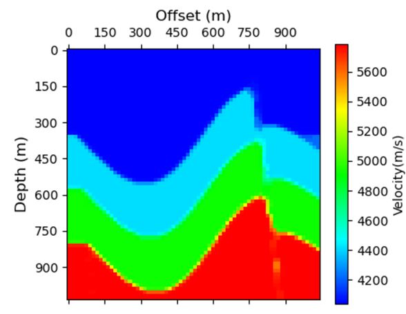
Under review as a conference paper at ICLR 2022
Dataset Supervision Method MAE ↓ MSE ↓ SSIM ↑
InversionNet 15.83 2156.00 0.9832
Supervised VelocityGAN 16.15 1770.31 0.9857
FlatFault H-PGNN+ 12.91 1565.02 0.9874
(our implementation)
UPFWI-24K (ours) 16.27 1705.35 0.9866
Unsupervised
UPFWI-48K (ours) 14.60 1146.09 0.9895
InversionNet 23.77 5285.38 0.9681
Supervised VelocityGAN 25.83 5076.79 0.9699
CurvedFault H-PGNN+ 24.19 5139.60 0.9685
(our implementation)
UPFWI-24K (ours) 29.59 5712.25 0.9652
Unsupervised
UPFWI-48K (ours) 23.56 3639.96 0.9756
Table 1: Quantitative results evaluated on OpenFWI in terms of MAE, MSE and SSIM. Our
UPFWI yields comparable inversion accuracy comparing to supervised baselines. For H-PGNN+,
we use our network architecture to replace the original one reported in their paper, and an additional
perceptual loss between seismic data is added during training.
set to be 4 × 10⁻⁵ , and we reduce the learning rate by a factor of 10 when validation loss reaches
a plateau. The minimum learning rate is set to be 4 × 10⁻⁷ . The size of mini-batch is set to be 16.
All trade-off hyper-parameters λ in our loss function are set to be 1. We implement our models in
Pytorch and train them on 8 NVIDIA Tesla V100 GPUs. All models are randomly initialized.
Evaluation Metrics: We consider three metrics for evaluating the velocity maps inverted by our
method: MAE, MSE and Structural Similarity (SSIM). Both MAE and MSE have been employed in
the existing methods (Wu & Lin, 2019; Zhang & Lin, 2020) to measure the pixel-wise error. Consid-
ering that the layered-structured velocity maps contain highly structured information, degradation or
distortion in velocity maps can be easily perceived by a human. To better align with human vision,
we employ SSIM to measure the perceptual similarity. It is important to note that for MAE and MSE
calculation, we denormalize velocity maps to their original scale while we keep them in normalized
scale [-1, 1] for SSIM according to the algorithm.
Comparison: We compare our method with three state-of-the-art algorithms: two pure data-driven
methods, i.e., InversionNet (Wu & Lin, 2019) and VelocityGAN (Zhang & Lin, 2020), and a physics-
informed method H-PGNN (Sun et al., 2021). We follow the implementation described in these
papers and search for the best hyper-parameters for OpenFWI dataset. Note that we improve H-
PGNN by replacing the network architecture with the CNN in our UPFWI and adding perceptual
loss, resulting in a significant boosted performance. We refer our implementation as H-PGNN+,
which is a strong supervised baseline. Our method has two variants (UPFWI-24K and UPFWI-
48K), using 24K and 48K unlabeled seismic data respectively.
5.2 M AIN R ESULTS
Results on FlatFault: Table 1 shows the results of different methods on FlatFault. Compared to
data-driven InversionNet and VelocityGAN, our UPFWI-24K performs better in MSE and SSIM,
but is slightly worse in MAE score. Compared to the physics-informed H-PGNN+, there is a gap
between our UPFWI-24K and H-PGNN+ when trained with the same amount of data. However,
after we double the size of unlabeled data (from 24K to 48K), a significant improvement is observed
in our UPFWI-48K for all three metrics, and it outperforms all three supervised baselines in MSE
and SSIM. This demonstrates the potential of our UPFWI for achieving higher performance with
more unlabeled data involved.
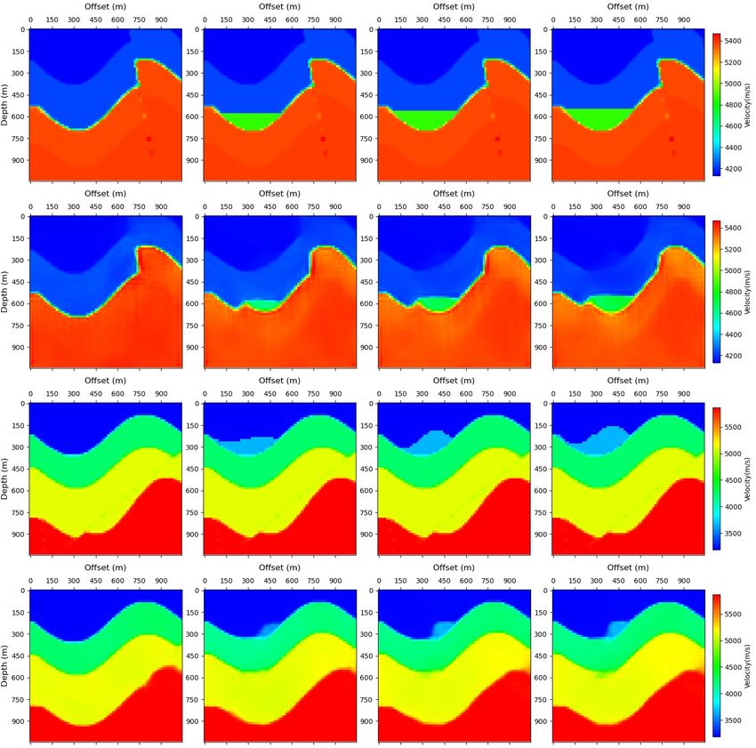
The velocity maps inverted by different methods are shown in Figure 4. Consistent with our quanti-
tative analysis, more accurate details are observed in the velocity maps generated by UPFWI-48K.
For instance, in the first row of Figure 4, although all models somehow reveal the small geophysical
6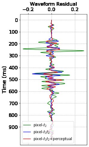
Under review as a conference paper at ICLR 2022

                                                                   UPFWI-24K      UPFWI-48K
   Ground Truth     InversionNet   VelocityGAN       H-PGNN+
                                                                     (Ours)          (Ours)

Figure 4: Comparison of different methods on inverted velocity maps of FlatFault. Our UPFWI-
48K reveals more accurate details at layer boundaries and the slope of the fault in deep region.

                                                                   UPFWI-24K      UPFWI-48K
   Ground Truth     InversionNet   VelocityGAN       H-PGNN+
                                                                     (Ours)          (Ours)

Figure 5: Comparison of different methods on inverted velocity maps of CurvedFault. Our
UPFWI reconstructs the geological anomalies on the surface that best match the ground truth.

fault near to the right boundary of the velocity map, only UPFWI-48K reconstructs a clear interface
between layers as highlighted by the yellow square. In the second row, we find both Inversion-
Net and VelocityGAN generate blurry results in deep region, while H-PGNN+, UPFWI-24K and
UPFWI-48K yield much clearer boundaries. We attribute this finding as the impact of seismic loss.
We further observe that the slope of the fault in deep region is different from that in the shallow
region, yet only UPFWI-48K replicates this result as highlighted by the green square.
Results on CurvedFault Table 1 shows the results of CurvedFault. Performance degradation is ob-
served for all models, due to the more complicated geological structures in CurvedFault. Although
our UPFWI-24K underperforms the three supervised baselines, our UPFWI-48K significantly boosts
the performance, outperforming all supervised methods in terms of all three metrics. This demon-
strates the power of unsupervised learning in our UPFWI that greatly benefits from more unlabeled
data when dealing with more complicated curved structure.
Figure 5 shows the visualized velocity maps in CurvedFault obtained using different methods. Sim-
ilar to the observation in FlatFault, our UPFWI-48K yields more accurate details compared to the
results of supervised methods. For instance, in the first row, only our UPFWI-24K and UPFWI-48K
precisely reconstruct the fault beneath the curve around the top-left corner as highlighted by the
yellow square. Although some artifacts are observed in the results of UPFWI-24K around the layer
boundary in deep region, they are eliminated in the results of UPFWI-48K. As for the example in the
second row, it is obvious that the shape of geological anomalies in the shallow region is best recon-
structed by our UPFWI-24K and UPFWI-48K as highlighted by the red square. More visualization
results are shown in the Appendix.

                                                 7
Under review as a conference paper at ICLR 2022
pixel-`1 `2
Ground Truth pixel-`2 pixel-`1 `2
+ perceptual
(a) (b)
Figure 6: Comparison of UPFWI with different loss functions on (a) waveform residual and
their corresponding inversion results (ground truth provided in the first column), and (b) single trace
residuals recorded by the receiver at 525 m offset. Our UPFWI trained with pixel-wise loss (`1 +`2
distance) and perceptual loss yields the most accurate results. Best viewed in color.
Loss Velocity Error Seismic Error
pixel-`2 pixel-`1 perceptual MAE ↓ MSE ↓ SSIM ↑ MAE ↓ MSE ↓ SSIM ↑
X 32.61 10014.47 0.9735 0.0167 0.0023 0.9978
X X 21.71 2999.55 0.9775 0.0155 0.0025 0.9977
X X X 16.27 1705.35 0.9866 0.0140 0.0021 0.9984
Table 2: Quantitative results of our UPFWI with different loss function settings in terms of
MAE, MSE and SSIM. Both the pixel-wise loss computed in `1 distance and perceptual loss con-
tribute to the boost of performance.
5.3 A BLATION S TUDY
Below we study the contribution of different loss functions: (a) pixel-wise `2 distance (MSE), (b)
pixel-wise `1 distance (MAE), and (c) perceptual loss. All experiments are conducted on FlatFault
using 24,000 unlabeled data.
Figure 6a shows the predicted velocity maps for using three loss combinations (pixel-`2 , pixel-`1 `2 ,
pixel-`1 `2 +perceptual) in UPFWI. The ground truth seismic data and velocity map are shown in the
left column. For each loss option, we show the difference between the reconstructed and the input
seismic data (on the top) and predicted velocity (on the bottom). When using pixel-wise loss in l2
distance alone, there are some obvious artifacts in both seismic data (around 600 millisecond) and
velocity map. These artifacts are mitigated by introducing additional pixel-wise loss in l1 distance.
With perceptual loss added, more details are correctly retained (e.g. seismic data from 400 millisec-
ond to 600 millisecond, velocity boundary between layers). Figure 6b compares the reconstructed
seismic data (in terms of residual to the ground truth) at a slice of 525 meter offset (orange dash line
in Figure 6a). Clearly, the combination of pixel-wise and perceptual loss has the smallest residual.
The quantitative results are shown in Table 2. They are consistent with the observation in qualitative
analysis (Figure 6a). In particular, using pixel-wise loss in l2 distance has the worst performance.
The involvement of `1 distance mitigates all velocity errors but is slightly worse on MSE and SSIM
of seismic error. Adding perceptual loss further boosts the performance in all performance metrics
by a clear margin. This shows that perceptual loss is helpful to retain waveform coherence, which is
correlated to the velocity boundary, and validates our proposed loss function (combining pixel-wise
and perceptual loss).
8Under review as a conference paper at ICLR 2022
6 D ISCUSSION
Our UPFWI has two major limitations. Firstly, it needs further improvement on a small number
of challenging velocity maps where adjacent layers have very close velocity values. We find that
the lack of supervision is not the cause as our UPFWI can yield comparable or even better results
compared to its supervised counterparts. Another limitation is the speed and memory consumption
for forward modeling, as the gradient of finite difference (see Equation 6) need to be stored for
backpropagation. We will explore different loss functions (e.g. adversarial loss) and the methods
that can balance the requirement of computation resources and the accuracy in the future work.
We believe the idea of connecting CNN and PDE to solve full waveform inversion has potential
to be applied to other inverse problems with a governing PDE such as medical imaging and flow
estimation.
7 R ELATED W ORK
Physics-driven Methods There are two primary physics-driven methods, depending on the com-
plexity of the forward model. The simpler one is via travel time inversion (Tarantola, 2005), which
has a linear forward operator, but provides results of inferior accuracy (Lin et al., 2015). FWI tech-
niques (Virieux & Operto, 2009), being the other one, provide superior solutions by modeling the
wave propagation, but the forward operator is non-linear and computationally expensive. Further-
more the problem is ill-posed (Virieux & Operto, 2009), making a prior model of the solution space
essential. Since regularized FWI solved via iterative techniques need to apply the forward model
many times, these solutions are very computationally expensive. In addition, existing regularized
FWI methods employ relatively simplistic models of the solution space (Hu et al., 2009; Burstedde
& Ghattas, 2009; Ramı́rez & Lewis, 2010; Lin & Huang, 2017; 2015b;a; Guitton, 2012; Treister &
Haber, 2016), leaving considerable room for improvement in the accuracy of the solutions. Another
common approach to alleviate the ill-posedness and non-linearity of FWI is via multi-scale tech-
niques (Bunks et al., 1995; Boonyasiriwat et al., 2009). Rather than matching the seismic data all at
once, the multi-scale techniques decompose the data into different frequency bands so that the low-
frequency components will be updated first and then followed with higher frequency components.
Data-driven Methods Recently, a new type of methods has been developed based on deep learning.
Araya-Polo et al. (2018) proposed a model based on a fully connected network. Wu & Lin (2019)
further converted FWI into an image-to-image translation task with an encoder-decoder structure
that can handle more complex velocity maps. Zhang & Lin (2020) adopted GAN and transfer learn-
ing to improve the generalization. Li et al. (2020) designed SeisInvNet to solve the misaligned issue
when dealing sources from different locations. In Yang & Ma (2019), a U-Net architecture was pro-
posed with skip connections. Feng et al. (2021) proposed a data-driven multi-scale framework by
considering different frequency components. Rojas-Gómez et al. (2020) developed an adaptive data
augmentation method to improve the generalization. Ren et al. (2020) combined the data-driven
and physics-based methods and proposed H-PGNN model. Some similar ideas were developed on
different physical forward models. Wang et al. (2020) proposed a model by connecting two CNNs
approximating the forward model and inversion process, and their model was tested on well-logging
data. Alfarraj & AlRegib (2019) utilized the forward model to constrain the training of convolutional
and recurrent neural layers to invert well-logging seismic data for elastic impedance. All of those
aforementioned works were developed based on supervised learning. Biswas et al. (2019) designed
an unsupervised CNN to estimate subsurface reflectivity using pre-stack seismic angle gather. Com-
paring to FWI, their problem is simpler because of the approximated and linearized forward model.
8 C ONCLUSION
In this study, we introduce an unsupervised method named UPFWI to solve FWI by connecting CNN
and forward modeling in a loop. Our method can learn the inverse mapping from seismic data alone
in an end-to-end manner. We demonstrate through a series of experiments that our UPFWI trained
with sufficient amount of unlabeled data outperforms the supervised counterpart on our dataset to
be released. The ablation study further substantiates that perceptual loss is a critical component in
our loss function and has a great contribution to the performance of our UPFWI.
9Under review as a conference paper at ICLR 2022
R EFERENCES
Amir Adler, Mauricio Araya-Polo, and Tomaso Poggio. Deep learning for seismic inverse problems:
toward the acceleration of geophysical analysis workflows. IEEE Signal Processing Magazine,
38(2):89–119, 2021.
Motaz Alfarraj and Ghassan AlRegib. Semisupervised sequence modeling for elastic impedance
inversion. Interpretation, 7(3):SE237–SE249, 2019.
Mauricio Araya-Polo, Joseph Jennings, Amir Adler, and Taylor Dahlke. Deep-learning tomography.
The Leading Edge, 37(1):58–66, 2018.
Reetam Biswas, Mrinal K Sen, Vishal Das, and Tapan Mukerji. Prestack and poststack inversion
using a physics-guided convolutional neural network. Interpretation, 7(3):SE161–SE174, 2019.
Chaiwoot Boonyasiriwat, Paul Valasek, Partha Routh, Weiping Cao, Gerard T Schuster, and Brian
Macy. An efficient multiscale method for time-domain waveform tomography. Geophysics, 74
(6):WCC59–WCC68, 2009.
Carey Bunks, Fatimetou Saleck, S Zaleski, and G Chavent. Multiscale seismic waveform inversion.
Geophysics, 60(5):1457–1473, 1995.
Carsten Burstedde and Omar Ghattas. Algorithmic strategies for full waveform inversion: 1D ex-
periments. Geophysics, 74(6):37–46, 2009.
Francis Collino and Chrysoula Tsogka. Application of the perfectly matched absorbing layer model
to the linear elastodynamic problem in anisotropic heterogeneous media. Geophysics, 66(1):
294–307, 2001.
Alexey Dosovitskiy, Lucas Beyer, Alexander Kolesnikov, Dirk Weissenborn, Xiaohua Zhai, Thomas
Unterthiner, Mostafa Dehghani, Matthias Minderer, Georg Heigold, Sylvain Gelly, et al. An
image is worth 16x16 words: Transformers for image recognition at scale. In International
Conference on Learning Representations, 2020.
Shihang Feng, Youzuo Lin, and Brendt Wohlberg. Multiscale data-driven seismic full-waveform
inversion with field data study. IEEE Transactions on Geoscience and Remote Sensing, pp. 1–14,
2021. doi: 10.1109/TGRS.2021.3114101.
Antoine Guitton. Blocky regularization schemes for full waveform inversion. Geophysical
Prospecting, 60:870–884, 2012.
Wenyi Hu, Aria Abubakar, and Tarek Habashy. Simultaneous multifrequency inversion of full-
waveform seismic data. Geophysics, 74(2):1–14, 2009.
Sergey Ioffe and Christian Szegedy. Batch normalization: Accelerating deep network training by
reducing internal covariate shift. In International Conference on Machine Learning, pp. 448–456.
PMLR, 2015.
Justin Johnson, Alexandre Alahi, and Li Fei-Fei. Perceptual losses for real-time style transfer and
super-resolution. In European Conference on Computer Vision, pp. 694–711. Springer, 2016.
Alex Krizhevsky, Ilya Sutskever, and Geoffrey E Hinton. ImageNet classification with deep convo-
lutional neural networks. Advances in Neural Information Processing Systems, 25:1097–1105,
2012.
Shucai Li, Bin Liu, Yuxiao Ren, Yangkang Chen, Senlin Yang, Yunhai Wang, and Peng Jiang. Deep-
learning inversion of seismic data. IEEE Transactions on Geoscience and Remote Sensing, 58(3):
2135–2149, 2020. doi: 10.1109/TGRS.2019.2953473.
Youzuo Lin and Lianjie Huang. Acoustic- and elastic-waveform inversion using a modified Total-
Variation regularization scheme. Geophysical Journal International, 200(1):489–502, 2015a. doi:
10.1093/gji/ggu393.
10Under review as a conference paper at ICLR 2022
Youzuo Lin and Lianjie Huang. Quantifying subsurface geophysical properties changes using
double-difference seismic-waveform inversion with a modified Total-Variation regularization
scheme. Geophysical Journal International, 203(3):2125–2149, 2015b. doi: 10.1093/gji/ggv429.
Youzuo Lin and Lianjie Huang. Building subsurface velocity models with sharp interfaces using
interface-guided seismic full-waveform inversion. Pure and Applied Geophysics, 174(11):4035–
4055, 2017. doi: 10.1007/s00024-017-1628-5.
Youzuo Lin, Ellen M. Syracuse, Monica Maceira, Haijiang Zhang, and Carene Larmat. Double-
difference traveltime tomography with edge-preserving regularization and a priori interfaces.
Geophysical Journal International, 201(2):574, 2015. doi: 10.1093/gji/ggv047.
Ilya Loshchilov and Frank Hutter. Decoupled weight decay regularization. In International
Conference on Learning Representations, 2018.
Ben Moseley, Tarje Nissen-Meyer, and Andrew Markham. Deep learning for fast simulation of
seismic waves in complex media. Solid Earth, 11(4):1527–1549, 2020.
Vinod Nair and Geoffrey E Hinton. Rectified linear units improve restricted Boltzmann machines. In
Proceedings of the 27th International Conference on Machine Learning (ICML-10), pp. 807–814,
2010.
Adriana Ramı́rez and Winston Lewis. Regularization and full-waveform inversion: A two-step
approach. In 80th Annual International Meeting, SEG, Expanded Abstracts, pp. 2773–2778,
2010.
Yuxiao Ren, Xinji Xu, Senlin Yang, Lichao Nie, and Yangkang Chen. A physics-based neural-
network way to perform seismic full waveform inversion. IEEE Access, 8:112266–112277, 2020.
Renán Rojas-Gómez, Jihyun Yang, Youzuo Lin, James Theiler, and Brendt Wohlberg. Physics-
consistent data-driven waveform inversion with adaptive data augmentation. IEEE Geoscience
and Remote Sensing Letters, 2020.
Karen Simonyan and Andrew Zisserman. Very deep convolutional networks for large-scale image
recognition. In International Conference on Learning Representations, 2015.
Jian Sun, Kristopher A Innanen, and Chao Huang. Physics-guided deep learning for seismic inver-
sion with hybrid training and uncertainty analysis. Geophysics, 86(3):R303–R317, 2021.
Albert Tarantola. Inverse problem theory and methods for model parameter estimation. SIAM,
2005.
Ilya Tolstikhin, Neil Houlsby, Alexander Kolesnikov, Lucas Beyer, Xiaohua Zhai, Thomas Un-
terthiner, Jessica Yung, Andreas Peter Steiner, Daniel Keysers, Jakob Uszkoreit, et al. Mlp-mixer:
An all-mlp architecture for vision. In Thirty-Fifth Conference on Neural Information Processing
Systems, 2021.
Eran Treister and Eldad Haber. Full waveform inversion guided by travel time tomography. SIAM
Journal on Scientific Computing, 39:S587–S609, 2016.
Jean Virieux and Stéphane Operto. An overview of full-waveform inversion in exploration geo-
physics. Geophysics, 74(6):WCC1–WCC26, 2009.
Yanghua Wang. Frequencies of the Ricker wavelet. Geophysics, 80(2):A31–A37, 2015.
Yuqing Wang, Qiang Ge, Wenkai Lu, and Xinfei Yan. Well-logging constrained seismic inver-
sion based on closed-loop convolutional neural network. IEEE Transactions on Geoscience and
Remote Sensing, 58(8):5564–5574, 2020.
Yue Wu and Youzuo Lin. InversionNet: An efficient and accurate data-driven full waveform inver-
sion. IEEE Transactions on Computational Imaging, 6(1):419–433, 2019.
Fangshu Yang and Jianwei Ma. Deep-learning inversion: A next-generation seismic velocity model
building method. Geophysics, 84(4):R583–R599, 2019.
11Under review as a conference paper at ICLR 2022
Zhongping Zhang and Youzuo Lin. Data-driven seismic waveform inversion: A study on the robust-
ness and generalization. IEEE Transactions on Geoscience and Remote Sensing, 58:6900–6913,
2020.
A A PPENDIX
A.1 D ERIVATION OF F ORWARD M ODELING IN P RACTICE
Similar to the finite difference in time domain, in 2D situation, by applying the fourth-order central
finite difference in space, the Laplacian of p(r, t) can be discretized as
∂2p ∂2p
∇2 p(r, t) = + 2,
∂x2 ∂z
2 2
1 X
t 1 X (11)
≈ c i p x+i,z + ci pt
(∆x)2 i=−2 (∆z)2 i=−2 x,z+i
+ O[(∆x)4 + (∆z)4 ] ,
where c0 = − 25 , c1 = 34 , c2 = − 121
, ci = c−i , and x and z stand for the horizontal offset and the
depth of a 2D velocity map, respectively. For convenience, we assume that the vertical grid spacing
∆z is identical to the horizontal grid spacing ∆x.
Given the approximation in Equations 5 and 11, we can rewrite the Equation 1 as
2
X
pt+1 t t−1 2 t
x,z = (2 − 5α)px,z − px,z + (∆x) αsx,z + α ci (ptx+i,z + ptx,z+i ) , (12)
i=−2
i6=0
where α = ( v∆t 2
∆x ) .
During the simulation of the forward modeling, the boundaries of the velocity maps should be care-
fully handled because they may cause reflection artifacts that interfere with the desired waves. One
of the standard methods to reduce the boundary effects is to add absorbing layers around the original
velocity map. Waves are trapped and attenuated by a damping parameter when propagating through
those absorbing layers. Here, we follow Collino & Tsogka (2001) and implement the damping
parameter as
3uv
κ = d(u) = ln(R) , (13)
2L2
where L denotes the overall thickness of absorbing layers, u indicates the distance between the
current position and the closest boundary of the original velocity map, and R is the theoretical
reflection coefficient chosen to be 10−7 . With absorbing layers added, Equation 6 can be ultimately
written as
2
X
pt+1 t t−1 2 t
x,z = (2 − 5α − κ)px,z − (1 − κ)px,z + (∆x) αsx,z + α ci (ptx+i,z + ptx,z+i ) . (14)
i=−2
i6=0
A.2 O PEN FWI E XAMPLES AND I NVERSION R ESULTS OF D IFFERENT M ETHODS
12Under review as a conference paper at ICLR 2022
Seismic Measurements in Five Channels
Velocity Channel 1 Channel 2 Channel 3 Channel 4 Channel 5
Figure 7: More examples of velocity maps and their corresponding seismic measurements in Open-
FWI dataset.
13Under review as a conference paper at ICLR 2022
UPFWI-24K UPFWI-48K
Ground Truth InversionNet VelocityGAN H-PGNN+
(Ours) (Ours)
Figure 8: Comparison of different methods on inverted velocity maps of FlatFault. The details
revealed by our UPFWI are highlighted.
14Under review as a conference paper at ICLR 2022
UPFWI-24K UPFWI-48K
Ground Truth InversionNet VelocityGAN H-PGNN+
(Ours) (Ours)
Figure 9: Comparison of different methods on inverted velocity maps of CurvedFault. The details
revealed by our UPFWI are highlighted.
15Under review as a conference paper at ICLR 2022
Ground Truth Ground Truth Prediction Prediction
Figure 10: Results of low-resolution Marmousi Dataset. This dataset contains low-resolution
velocity maps generated using style tranfer with the Marmousi velocity map as the style images.
Our UPFWI model yields good results in shallow regions, and it also captures some geological
structures in deeper regions. Similar phenomenon is also observed in the prediction of the smoothed
Marmousi velocity map (bottom-right corner).
A.3 A DDITIONAL E XPERIMENT R ESULTS
Additional experiments on more challenging datasets (Marmousi & Salt datasets). We further
evaluate our UPFWI on two more challenging tests including Salt (Yang & Ma, 2019) and Marmousi
datasets and achieve solid results on both datasets. For Marmousi dataset, we follow the work of
Feng et al. (2021) and employ the Marmousi velocity map as the style image to construct a low-
resolution dataset with physically realistic subsurface velocity maps. The visualization of results on
Marmousi dataset and Salt data are shown in Figures 10 and 11, respectively. Table 3 further shows
the quantitative results on both datasets. Although our UPFWI achieves good results on Salt dataset
with preserved subsurface structures, it has clearly larger errors than the supervised InversionNet.
This is due to two reasons: (a) Salt dataset has a small amount of training data (120 samples),
which is very challenging for unsupervised methods; (b) the variability between training and testing
samples is small, providing a significantly larger favor to supervised methods than the unsupervised
counterparts.
Dataset Model MAE↓ MSE↓ SSIM↑
InversionNet 149.67 45936.23 0.7889
Marmousi
UPFWI 221.93 125825.75 0.7920
InversionNet 25.98 8669.98 0.9764
Salt
UPFWI 150.34 164595.28 0.7837
Table 3: Quantitative results evaluated on Marmousi and Salt.
16Under review as a conference paper at ICLR 2022
Ground Truth
Prediction
Figure 11: Results of salt bodies dataset. This dataset contains more complicated velocity map.
Our UPFWI model yields good velocity map prediction on both salt bodies and background geolog-
ical structures.
Additional experiments on more network architectures (Vision Transformer & MLP-Mixer).
We further conducted experiments by using Vision Transformer (ViT) (Dosovitskiy et al., 2020) and
MLP-Mixer (Tolstikhin et al., 2021) to replace CNN as the encoder. The visualization results are
shown in Figure 12. Table 4 further shows the quantitative results. Solid results are obtained for
both network architectures, indicating our proposed method is model-agnostic.
Network Architecture MAE↓ MSE↓ SSIM↑
CNN 16.27 1705.35 0.9866
ViT 41.44 11029.01 0.9461
MLP-Mixer 22.32 4177.37 0.9726
Table 4: Quantitative results of our UPFWI with different network architectures.
Additional experiments to investigate generalization. We conducted two additional experiments:
(1) training our model on the CurvedFault dataset and further testing on the FlatFault dataset (visu-
alization results are listed in Figure 13, and quantitative results are shown in Table 5); (2) testing our
model on time-lapse imaging problems (visualization results are listed in Figure 14). The results
demonstrate that our proposed model yields generalization ability to a certain degree.
Training Dataset Test Dataset MAE↓ MSE↓ SSIM↑
FlatFault FlatFault 14.60 1146.09 0.9895
CurvedFault FlatFault 50.80 17627.65 0.9253
Table 5: Quantitative results of our UPFWI models evaluated on FlatFault.
Additional experiments on noise handling. We validate the robustness of our UPFWI models by
two additional tests: (1) testing data contaminated by Gaussian noise and (2) testing data with some
missing traces. The visualization results of the first experiment are shown in Figures 15 and 16, and
the quantitative results are shown in Table 6. The visualization results of the second experiment are
shown in Figures 17 and 18, and the quantitative results are shown in Table 7. The results from
both experiments demonstrate that our model can be robust to a certain levels of noise and irregular
acquisition.
17Under review as a conference paper at ICLR 2022
Ground Truth CNN MLP-Mixer ViT
Figure 12: Results of UPFWI with different network architectures. We replace the CNN in our
model with Vision Transformer (ViT) and MLP-Mixer as the encoder and test them on the FlatFault
dataset. Both models yield reasonable velocity maps. This demonstrates that our proposed learning
paradigm is model-agnostic.
18Under review as a conference paper at ICLR 2022
Ground Truth
Prediction
Figure 13: Results on generalization across datasets. The test is performed on FlatFault by apply-
ing a UPFWI model that is trained on CurvedFault dataset. Although the artifact is not negligible,
the fault structures and velocity values are well preserved. This demonstrates that our model has
generalizability to a certain degree.
t=0 t=1 t=2 t=3
Ground Truth
Prediction
Ground Truth
Prediction
Figure 14: Results on generalizability over geological anomalies. The test is performed on a
dataset where we add additional geological anomalies to simulate time-lapse imaging problems.
The velocity maps containing those anomalies are not included during training. However, our model
captures the spatial and temporal dynamics of anomalies in prediction. This demonstrates that our
model has generalizability to a certain degree.
19Under review as a conference paper at ICLR 2022
Ground Truth Clean PSNR=61.60dB PSNR=58.70dB PSNR=51.58dB
Seismic Input
Velocity Map
Seismic Input
Velocity Map
Figure 15: Results of adding Gaussian noise to FlatFault. The model is trained on the clean data
(without noise) and tested on different levels (PSNR) of Gaussian noises. Clearly, our method is
robust to the noise although slight degradation is observed when noise level increases.
20Under review as a conference paper at ICLR 2022
Ground Truth Clean PSNR=61.72dB PSNR=58.70dB PSNR=51.68dB
Seismic Input
Velocity Map
Seismic Input
Velocity Map
Figure 16: Results of adding Gaussian noise to CurvedFault. The model is trained on the clean
data (without noise) and tested on different levels (PSNR) of Gaussian noises. Similar to the results
of FlatFault, our method is robust to the noise although slight degradation is observed when noise
level increases.
21Under review as a conference paper at ICLR 2022
Ground Truth Clean 7 Missing 10 Missing 17 Missing
Seismic Input
Velocity Map
Seismic Input
Velocity Map
Figure 17: Results of randomly missing traces on FlatFault. The model is trained on the clean
data (without missing traces) and tested on multiple missing rates from 5% to 25%. Our method is
robust to the missing traces. Although the higher missing rate leads to shifts in velocity values, the
geological structures are well preserved.
22Under review as a conference paper at ICLR 2022
Ground Truth Clean 7 Missing 10 Missing 17 Missing
Seismic Input
Velocity Map
Seismic Input
Velocity Map
Figure 18: Results of randomly missing traces on CurvedFault. The model is trained on the clean
data (without missing traces) and tested on multiple missing rates from 5% to 25%. Similar to the
results of FlatFault, our method is robust to the missing traces. Although the higher missing rate
leads to shifts in velocity values, the geological structures are well preserved.
23Under review as a conference paper at ICLR 2022
Dataset σ (10−4 ) PSNR MAE↓ MSE↓ SSIM↑
0 100 14.60 1146.09 0.9895
0.5 61.60 15.68 1343.21 0.9888
FlatFault
1.0 58.70 24.84 4010.78 0.9733
5.0 51.58 44.33 7592.57 0.9681
0 100 23.56 3639.96 0.9756
0.5 61.72 23.78 3704.00 0.9751
CurvedFault
1.0 58.70 24.84 4010.78 0.9733
5.0 51.68 46.90 10415.38 0.9441
Table 6: Quantitative results of our UPFWI tested on seismic inputs with different noise levels.
Dataset Missing Traces MAE↓ MSE↓ SSIM↑
0 14.60 1146.09 0.9895
4 (5%) 21.23 1772.05 0.9868
FlatFault
7 (10%) 33.66 3504.25 0.9814
17 (25%) 85.21 16731.69 0.9457
0 23.56 3639.96 0.9756
4 (5%) 41.33 6914.12 0.9622
CurvedFault
7 (10%) 61.72 12445.90 0.9453
17 (25%) 121.06 36770.77 0.8853
Table 7: Quantitative results of our UPFWI tested on seismic inputs with different numbers of
missing traces.
24You can also read