CONVERGENT GRAPH SOLVERS - OpenReview

Published as a conference paper at ICLR 2022

C ONVERGENT G RAPH S OLVERS
 Junyoung Park, Jinhyun Choo & Jinkyoo Park
 KAIST, Daejeon, South Korea
 {junyoungpark,jinhyun.choo,jinkyoo.park}@kaist.ac.kr

 A BSTRACT

 We propose the convergent graph solver (CGS)1 , a deep learning method that
 learns iterative mappings to predict the properties of a graph system at its stationary
 state (fixed point) with guaranteed convergence. The forward propagation of CGS
 proceeds in three steps: (1) constructing the input-dependent linear contracting
 iterative maps, (2) computing the fixed points of the iterative maps, and (3) decoding
 the fixed points to estimate the properties. The contractivity of the constructed
 linear maps guarantees the existence and uniqueness of the fixed points following
 the Banach fixed point theorem. To train CGS efficiently, we also derive a tractable
 analytical expression for its gradient by leveraging the implicit function theorem.
 We evaluate the performance of CGS by applying it to various network-analytic
 and graph benchmark problems. The results indicate that CGS has competitive
 capabilities for predicting the stationary properties of graph systems, irrespective
 of whether the target systems are linear or non-linear. CGS also shows high
 performance for graph classification problems where the existence or the meaning
 of a fixed point is hard to be clearly defined, which highlights the potential of CGS
 as a general graph neural network architecture.

1 I NTRODUCTION

Our world is replete with networked systems, where their overall properties emerge from complex
interactions among the system entities. Such networked systems attain their unique properties from
their stationary states; hence, finding these stationary properties is a common goal for many problems
that arise in the science and engineering field. Examples of such problems include the minimization
of the molecule’s potential energy that finds the stationary positions of the atoms to compute the
potential energy of the molecule (Moloi & Ali, 2005), the PageRank algorithm that finds the stationary
importance of online web pages to compute recommendation scores (Brin & Page, 1998), and the
network analysis of fluid flow in porous media that finds the stationary pressures in pore networks to
compute the macroscopic properties of the media (Gostick et al., 2016). In these network-analytic
problems, the network is often represented as a graph, and the stationary states are often computed
through a problem-specific iterative method derived analytically from the prior knowledge of the
target system. By applying the iterative map repeatedly, these methods compute the stationary states
(i.e., fixed points) and the associated properties of the target system. However, analytically deriving
such iterative maps for highly complex systems typically requires tremendous efforts and time.
Instead of deriving/designing the problem-specific iterative methods, researchers employ deep learn-
ing approaches to learn the iterative methods (Dai et al., 2018; Gu et al., 2020; Hsieh et al., 2019;
Huang et al., 2020). These approaches learn an iterative map directly without using domain-specific
knowledge, but using only the input and output data. By applying the learned iterative map, these
approaches (approximately) compute the fixed points and predict the properties of a target system.
Graph Neural Networks (GNNs) have been widely used to construct iterative maps (Dai et al., 2018;
Gu et al., 2020; Scarselli et al., 2008; Alet et al., 2019). However, when applying this approach,
the existence of the fixed points is seldom guaranteed. As a result, the number of iterative steps is
often required to be specified, as a hyperparameter, to ensure the termination of the iterations. This
may cause premature termination or inefficient backward propagation if the number of iterations is
inadequately small or too large.
 1
 The code is available at https://github.com/Junyoungpark/CGS.

 1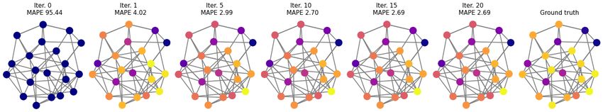

Published as a conference paper at ICLR 2022

In this study, we propose a convergent graph solver (CGS), a deep learning method that can predict
the solution of a target graph analytical problem using only the input and output data, and without
requiring the prior knowledge of existing solvers or intermediate solutions. The forward propagation
of CGS is designed to proceed in the following three steps:
 • Constructing the input-dependent linear-contracting iterative maps. CGS uses the input
 graph, which dictates the specification of the target network-analytic problem, to construct a set
 of linear contracting maps. This procedure formulates/set up the internal problem to be solved by
 considering the problem conditions and contexts (i.e., boundary conditions or initial conditions in
 PDE domains – the physical network problems). Furthermore, the input-dependent linear map
 can produce any size of transition map flexibly depending on the input size graph; thus helping
 the trained model to generalize over unseen problems with different sizes (size transferability).
 • Computing the fixed points via iterative methods. CGS constructs a set of linear contracting
 maps, each of which is guaranteed to have a unique fixed point that embeds the important features
 for conducting various end tasks. Thus, CGS computes the unique solutions of the constructed
 linear maps via iterative methods (or direct inversion) with convergence guarantee.
 • Decoding the fixed points to estimate the properties. By using a separate decoder architecture,
 we compute the fixed points in the latent space while expecting them to be an effective representa-
 tion that can improve the predictive performance of the model. This enables CGS to be used not
 only for finding the real fixed points (or its transportation) if they exist, but also for computing the
 "virtual fixed point" as a representation learning method in general prediction tasks.

The parameters of CGS are optimized with the gradient computed based on the implicit function theo-
rem, which requires O(1) memory usage when computing the gradient along with the iterative steps.
CGS is different from the other studies that solve the constrained optimization (with convergence
guarantee) (Gu et al., 2020; Scarselli et al., 2008; Tiezzi et al., 2020) in that it does not impose any
restriction when optimizing the parameters. Instead, CGS is inherently structured to have the unique
fixed points owing to the uses of the linear map. Note that the structural restriction is only in the form
of an iterative map; we can flexibly generate the coefficients of the linear map using any network (i.e.,
GNN) and utilize multiple linear maps to boost the representability.
We evaluate the performance of CGS using two types of paradigmatic network-analytic problems:
physical diffusion in networks and the Markov decision process, where the true labels indeed exist
and can be computed analytically using linear and non-linear iterative methods, respectively. We
also employ CGS to solve various graph classification benchmark tasks to show that CGS can serve
as a general (implicit) layer like other GNN networks when conducting typical graph classification
tasks. In these experiments, we seek to compute a virtual fixed point that can serve as the best
hidden representation of the input when predicting the output. The results show that CGS can be (1)
an effective solver for graph network problems or (2) an effective general computational layer for
processing graph-structured data.

2 R ELATED W ORK

Convergent neural models. Previous studies that have attempted to achieve the convergence
property of neural network embedding (e.g., hidden vectors of MLP and hidden states of recurrent
neural networks) can be grouped into two categories: soft and hard approaches. Soft approaches
typically attain the desired convergence properties by augmenting the loss functions (Erichson
et al., 2019; Miyato et al., 2018). Although the soft approaches are network-architecture agnostic,
these methods cannot guarantee the convergence of the learned mappings. On the other hand, hard
approaches seek to guarantee the convergence of the iterative maps by restricting their parameters in
certain ranges (Gu et al., 2020; Tiezzi et al., 2020; Miller & Hardt, 2018; Kolter & Manek, 2019).
This is achieved by projecting the parameters of the models into stable regions. However, such
projection may lead to non-optimal performances since it is performed after the gradient update, i.e.,
the projection is disentangled from training objective.
Implicit deep models. The forward propagation of CGS, which solves fixed point iterations, is
closely related to deep implicit models. Instead of defining the computational procedures (e.g., the
depth of layer in neural network) explicitly, these models use implicit layers, which accept input-
dependent equations and compute the solutions of the input equations, for the forward propagation.

 2

Published as a conference paper at ICLR 2022

For instance, neural ordinary differential equations (NODE) (Chen et al., 2018; Massaroli et al.,
2020) solve ODE until the solver tolerance is satisfied or the integration domain is covered, the
optimization layers (Gould et al., 2016; Amos & Kolter, 2017) solve the optimization problem
until the duality gap converges, and the fixed point models (Bai et al., 2019; Winston & Kolter,
2020) solve the network-generated fixed point iterations until some numerical solver satisfy the
convergence condition. Implicit models use these (intermediate) solutions to conduct various end
tasks (e.g., regressions, or classifications). In this way, implicit models can impose desired behavioral
characteristics into layers as inductive bias and hence, often show superior parameter/memory
efficiency and predictability.
Fixed points of graph convolution. Methods that find the fixed points of graph convolutions have
been suggested in various contexts of graph-related tasks. Several works have utilized GNN along
with RNN-like connections to (approximately) find the fixed points of graph convolutions (Liao et al.,
2018; Dai et al., 2018; Li et al., 2015; Scarselli et al., 2008). Some have suggested to constrain the
parameter space of GNN so that the trained GNN becomes a non-expansive map, thus producing the
fixed point (Gu et al., 2020; Tiezzi et al., 2020). Others have proposed to apply an additional GNN
layer on the embedded graph and penalize the difference between the output of the additional GNN
layer and the embedded graph to guide the GNN to find the fixed points (Scarselli et al., 2008; Yang
et al., 2021). It has been shown that regularizing GNN to find its fixed points improves the predictive
performance (Tiezzi et al., 2020; Yang et al., 2021).
Comparison between CGS and existing approaches. Combining the ideas of (1) computing/using
the fixed points of the graph convolution (as a representation learning) and (2) utilizing the implicit
differentiation of the model (as a training method) has been proposed by numerous studies (Scarselli
et al., 2008; Liao et al., 2018; Johnson et al., 2020; Dai et al., 2018; Bai et al., 2019; Gallicchio
& Micheli, 2020; Bai et al., 2019; Tiezzi et al., 2020; Gu et al., 2020). Majority of those studies
assume that the convolution operators (iterative map) induce a convergent sequence of the (hidden)
representation; however, this assumption typically does not hold unless certain conditions hold
for the convolution operator (iterative map). When neither the convergence nor uniqueness holds,
it can possibly introduce biases in the gradient computed by implicit differentiation (Liao et al.,
2018; Blondel et al., 2021). Hence, to impose convergence, some methods restrict the learned
convolutions to be strictly contractive (i.e., the hidden solutions are convergent) by projecting the
learned parameters into a certain region and solving the constraint training problems, respectively
(Gu et al., 2020; Tiezzi et al., 2020). Unlike these methods restricting the parameters of the graph
convolutions directly, CGS guarantees the convergence and the uniqueness of the fixed point by
imposing the structural inductive bias on the iterative map, i.e., using the contractive linear map that
has a unique fixed point, thus alleviating the need to solve the constrained parameter optimization
(Tiezzi et al., 2020).

3 P ROBLEM D ESCRIPTION

The objective of many network-analytic problems can be described as:

 Find a solution vector Y ∗ from a graph G that represents the target network system.

In this section, we briefly explain a general iterative scheme to compute Y ∗ from G. The problem
specification G = (V, E) is a directed graph that is composed of a set of nodes V and a set of edges
E. We define the ith node as vi and the edge from vi to vj as eij . The general scheme of the iterative
methods is given as follows:

 H [0] = f (G), (1)
 [n] [n−1]
 H = T (H ; G), n = 1, 2, ... (2)
 [n] [n]
 Y = g(H ; G), n = 0, 1, ... (3)
where f (·) is the problem-specific initialization scheme that transforms G into the initial hidden
embedding H [0] , T is the problem-specific iterative map that updates the hidden embedding H [n]
from the previous embedding H [n−1] , and g(·) is the problem-specific decoding function that predicts
the intermediate solution Y [n] .

 3

Published as a conference paper at ICLR 2022

 ⋯ ⋯
 " "

 Fixed points aggregation
 Multi-head extension
 [ ] [ ] [ ] [ ' ]
 = + = + ∗ = ∗ + 

 ⋯
 ⋯

 ⋯

 ⋯

 ⋯
 ⋯ ⋯
 [ ] [ ]
 = + 
 [ ]
 = 
 [ ' ]
 + ∗ = ∗ + 
 = , ′, ′

 ⋯
 
 ⋯

 ⋯

 ⋯
 ⋯
 ⋯ ⋯
 [ ] [ ]
 = + 
 [ ]
 = 
 [ ' ]
 + ∗ = ∗ + 

 4.1 Constructing iterative maps 4.2 Computing fixed points 4.3 Decoding fixed points

Figure 1: Overview of forward propagation of CGS. Given an input graph G, the parameter-
 ∗
generating network fθ constructs contracting linear transition maps Tθ . The fixed points Hm of
Tθ are then computed via matrix inversion. The fixed points are aggregated into H ∗ , and then the
decoder gθ decodes H ∗ to produce Y ∗ .

T is designed such that the fixed point iteration (equation 2) converges to the unique fixed point H ∗ :

 lim H [n] = H ∗ s.t. H ∗ = T (H ∗ , G) (4)
 n→∞

The solution Y ∗ is then obtained by decoding H ∗ , i.e., g(H ∗ ; G) ≜ Y ∗ .
In many real-world network-analytic problems, we can obtain G and its corresponding solution Y ∗ ,
but not T , H [n] and Y [n] . Therefore, we aim to learn a mapping T from G to Y ∗ without using T ,
H [n] and Y [n] .

3.1 E XAMPLE : G RAPH VALUE I TERATION

Let us consider a finite Markov decision process (MDP), whose goal is to find the state values through
the iterative applications of the Bellman optimality backup operator (Bellman, 1954). We assume
that the state transition is deterministic.
We define G = (V, E), where V and E are the set of states and transitions of MDP respectively. vi
corresponds to the ith state of the MDP, and eij corresponds to the state transition from state i to j.
eij exists only if the state transition from state i to j is allowed in the MDP. The features of eij are
the corresponding state transition rewards. The objective is to find the state values V ∗ . In this setting,
the Bellman optimal backup operator T is defined as follows:
 [n] [n−1]
 Vi = T (V [n−1] ; G) ≜ max (rij + αVj ) (5)
 j∈N (i)

 [n]
where Vi is the state value of vi estimated at n-th iteration, N (i) is the set of states that can be
reached from the ith state via one step transition, rij is the immediate reward related to eij , and α is
the discount rate of the MDP.
In this graph value iteration (GVI) problem, the initial values V [0] are set as zeros (i.e., f (·) = 0),
then T is applied until V [n] converges, and V [n] is decoded with the identity mapping (i.e., g(·) is
identity and H [n] ≜ V [n] ). We will show how CGS constructs the transition map T from the input
graph and predicts the converged state values V ∗ without using equation 5 in the following sections.

4 C ONVERGENT G RAPH S OLVERS

We propose CGS that predicts the solution Y ∗ from the given input graph G in three steps: (1)
constructing linear iterative maps Tθ from G, (2) computing the unique fixed points H ∗ of Tθ via
iterative methods, and (3) decoding H ∗ to produce Y ∗ , as shown in Figure 1.

 4

Published as a conference paper at ICLR 2022

4.1 C ONSTRUCTING LINEAR ITERATIVE MAPS

CGS first constructs an input-dependent contracting linear map Tθ (· ; G) such that the repeated
application of Tθ (· ; G) always produces the unique fixed point H ∗ (i.e. limn→∞ H [n] = H ∗ ) that
embeds the essential characteristics of the input graph G for conducting end tasks. In other words,
CGS learns to construct iterative maps that are tailored to each input graph G, from which the unique
fixed points of the target system are guaranteed to be computed and used for conducting end tasks.
To impose the contraction property on the linear map, CGS utilizes the following iterative map:
 Tθ (H [n] ; G) ≜ γAθ (G)H [n] + Bθ (G) (6)
where γ is the contraction factor, Aθ (G) ∈ Rp×p is the input-dependent transition parameter,
Bθ (G) ∈ Rp is the input-dependent bias parameter, and p is the number of nodes in graph.
To construct an input-dependent iterative map that preserves the structural constraints, which is
required to guarantee the existence and uniqueness of a fixed point, we employ GNN-based parameter-
generating network fθ (·). The parameter generation procedure for Tθ starts by encoding G = (V, E):
 V′ , E′ = fθ (V, E) (7)
 ′ ′
 vi′
where V and E are the set of updated node embeddings ∈ R and edge embeddings q
 ∈R e′ij
respectively. CGS then constructs Aθ (G) by computing the (i, j)th element of Aθ (G) as follows:
 ( ′
 σ(eij )
 d(i) if eij exists,
 [Aθ (G)]i,j = (8)
 0 otherwise.
where σ(x) is a differentiable bounded function that projects x into the range [0, 1] (e.g., Sigmoid
function), and d(i) is the outward degree of vi (i.e.„ the number of outward edges of vi ). Bθ (G) is
simply constructed by vectorizing the updated node embeddings as [Bθ (G)]i,: = vi′ .
Theorem 1. The existence and uniqueness of H ∗ induced by Tθ (H [n] ; G). The proposed scheme for
constructing Aθ (G), along with the bounded contraction factor 0 < γ < 1, is sufficient for
Tθ (H [n] ; G) to be γ-contracting and, as a result, Tθ has unique fixed point H ∗ . Refer to Appendix
A.1 for the proof.
Multi-head extension. Tθ can be considered as a graph convolution layer defined in equation 6. Thus,
CGS can be easily extended to multiple convolutions in order to model a more complex iterative map.
To achieve such multi-head extension with M graph convolutions, one can design fθ to produce a set
of transition parameters [A1 , ..., Am , ..., AM ] and a set of bias parameters [B1 , ..., Bm , ..., BM ] for
 [n] [n]
Tm (Hm ; G) ≜ γAm Hm + Bm for m = 1, ..., M .

4.2 C OMPUTING FIXED POINTS
 ∗ [n] [n]
The fixed point Hm of the constructed iterative map Tm (Hm ; G) ≜ γAm Hm + Bm satisfies
 ∗ ∗
Hm = γAm Hm + Bm for m = 1, ..., M . Due to the linearity, we can compute the fixed point of
Tm via matrix inversion:
 ∗
 Hm = (I − γAm )−1 Bm (9)
where I ∈ Rp×p is the identity matrix. The existence of (I − γAm )−1 is assured from the fact
that Tm is contracting (see Appendix A.2). The matrix inversions can be found by applying various
automatic differentiation tools while maintaining its differentiability. However, the computational
complexity of the matrix inversion scales O(p3 ), which can limit this approach from being scaled to
large scale problems favorably.
To scale CGS to larger graph inputs, we compute the fixed point of Tm by repeatedly applying the
 [0]
iterative map Tm starting from an arbitrary initial hidden state Hm ∈ Rp until the hidden embedding
 [n] ∗
converges, i.e., limn→∞ Hm = Hm .
One can choose a way to compute the fixed point between inversion and iterative methods depending
on the size of the transition matrix Am and its sparsity because these factors can result in different
computational speed and accuracy. In general, for small-sized problems, inversion methods can be
favorable; while for large-sized problems, iterative methods are more efficient. (See Appendix D.6)

 5

Published as a conference paper at ICLR 2022

4.3 D ECODING FIXED POINTS

The final step of CGS is to aggregate the fixed points of multiple iterative maps and decode the
aggregated fixed points to produce Y ∗ . The entire decoding step is given as follows:
 H ∗ = [Hm
 ∗ ∗
 || ... ||HM ] (10)
 ∗ ∗
 Y = gϕ (H ; G) (11)
where H ∗ is the aggregated fixed points, M is the number of heads, and gϕ (·) is the decoder which
is analogous to the decoding function of the network-analytic problems (equation 3).

5 T RAINING CGS
To train CGS with gradient descent, we need to calculate the partial derivatives of the scalar-valued
loss L with respect to the parameters of Tθ . To do so, we express the partial derivatives using chain
rule taking H ∗ as the intermediate variable
 ∂L ∂L ∂H ∗
 = (12)
 ∂(·) ∂H ∗ ∂(·)
 ∂L
where (·) denotes the parameters of Aθ (G) or Bθ (G). Here, ∂H ∗ is readily computable via an
 ∂H ∗
automatic differentiation package. However, computing ∂(·) is less straightforward since H ∗ and
(·) are implicitly related via equation 6. One possible option to compute the partial derivatives is to
backpropagate through the iteration steps.
Although this approach can be easily employed using most automatic differentiation tools, it entails
extensive memory usage. Instead, exploiting the stationarity of H ∗ , we can derive an analytical
expression for the partial derivative using the implicit function theorem as follows:
 !−1
 ∂H ∗ ∂g(H ∗ , A, B) ∂g(H ∗ , A, B)
 =− (13)
 ∂(·) ∂H ∗ ∂(·)
where g(H, A, B) = H − (γAH + B). Here, we omit the input-dependency of A and B for
notational brevity. We compute the inverse terms via an iterative method. This option allows one to
train CGS with constant memory consumption over the iterative steps. The derivation of the partial
derivatives and the software implementation of equation 13 are provided in Appendix A.3 and B
respectively.

6 E XPERIMENTS
We first evaluate the performance of CGS for two types of network-analytic problems: (1) the
stationary state of physical diffusion in networks where the true solutions can be computed from
linear iterative maps, and (2) the state values via GVI where the true solutions can be calculated from
non-linear iterative maps. We then assess the capabilities of CGS as a general GNN layer by applying
CGS to solve several graph property prediction benchmarks problems.

6.1 P HYSICAL DIFFUSION IN NETWORKS

Diffusion of fluid, heat, and other physical quantities are omnipresent in the science and engineering
applications. Mathematically, physical diffusion in networks (e.g. pipe/pore networks) is often
described by a graph. The stationary state of the graph can be expressed as
 X
 kij (pi − pj ) = 0, ∀vi ∈ V \ ∂(V), (14)
 j∈N (i)

 pi = pbi , ∀vi ∈ ∂(V), (15)
where pi and pj are the potentials at vi and vj respectively, kij is the conductance of the edge the
connects the two nodes, and pbi is the prescribed potentials at the boundary nodes that belong to the
set ∂(V). Equation 14 specializes to a particular diffusion problem according to how p is prescribed
(e.g. pressure for fluid flow, and temperature for heat transfer).

 6

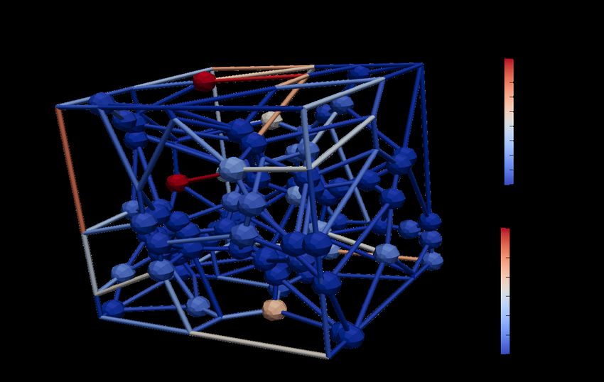
Published as a conference paper at ICLR 2022

 CGS(4) CGS(8) CGS(16) IGNN SSE GNN(1) GNN(2) GNN(3)
 CGS(4) CGS(16) SSE GNN(2)
 0.030 CGS(8) IGNN GNN(1) GNN(3)

 0.025
 0.0275
 0.020
 0.0250
MSE

 0.015 0.0225

 MSE
 0.010 0.0200
 0.0175
 0.005
 0.0150
 200 300 400 500 600 700 800 0.0125
 Number of Pores 0.0100

 1 2 3
Figure 2: Diffusion experiment results. The x- and y- Number of GNN layers

axis are the number of pores and the average MSE of the
test graphs. The error bars indicates the standard error of Figure 3: Number of GNN layers
predictions (measured from 500 instances per each size). vs. MSE (ns = 800).

As an example of physical diffusion, we consider
fluid flow in porous media – particularly, finding the
fluid pressures of a pore network that is in equilibrium
state (the solutions of equations 14 and 15). We
model the pore network as a 3D graph whose nodes
and edges correspond to pore chambers and throats
respectively as shown in figure 4. We assume linear
diffusion such that p (i.e., Y ∗ ) can be computed using
a linear iterative map (Gostick et al., 2016).
We employ CGS to predict the equilibrium pressures
Y ∗ inside pore networks G. The node features are the
Cartesian coordinates, volume, diameter, and bound-
ary indicator of its corresponding pore. The boundary
pressure is also as a node feature if the node corre- Figure 4: Pore network graph
sponds to a boundary pore. The edge features are the
cylinder volume, diameter, and length of its corre-
sponding throat. We sample training graphs such that the graphs fit into 0.1 m3 cubes. The training
graphs, which have 50–200 nodes, are then randomly generated (See Appendix C.1). We train CGS
such that it minimizes the mean-squared error (MSE) between the predicted ones and Y ∗ .
To investigate the effectiveness of the multi-head extension, we train CGS(4), CGS(8) and CGS(16),
where CGS(m) denotes CGS with m heads. For the baseline models, we use implicit GNNs, IGNN,
(Gu et al., 2020), SSE (Dai et al., 2018), and n-layer GNN models GNN(n). IGNN and SSE find the
fixed points in the forward propagation step. We utilize the same GNN architecture as the encoders
for all baselines except for SSE. Please refer to Appendix C.1 for the details about the data generation,
network architectures, and training schemes.
All CGS models show better generalization capabilities than the baselines in predicting Y ∗ as shown in
Figure 2, even though all models show similar prediction errors during training (See Appendix C.1.2).
CGSs with higher m show superior prediction results for the test cases. This difference evinces
that the use of multi-head extension (i.e., multiple linear iterative maps) is advantageous due to the
increased expressivity. Also, when comparing CGS(8) and GNN(1), which utilize the same encoder
architecture and thus has the same number of GNN layers as shown in Figure 3, CGS(8) shows better
prediction performance. This is because the 1-hop aggregation cannot provide enough information to
compute the equilibrium pressure. This result indicates that CGS successfully accommodates the
long-range patterns in graphs without adopting additional graph convolution layers.

6.2 G RAPH VALUE ITERATION

We investigate the performance of CGS on graph value iteration (GVI) problems, where the iterative
map (equation 5) is non-linear as explained in section 3.1. The goal of the experiments is to show
that CGS can estimate the state values that are computed from the nonlinear iterative map accurately,
even when using the set of learned linear iterative maps, as shown in figure 5.

 7

Published as a conference paper at ICLR 2022

Figure 5: Solutions of GVI with CGS. The balls represent the states of MDP and the ball colors show
the prediction results and their corresponding targets. More details are described in the main text.

Table 1: Graph Value Iteration results. We report the average MAPE and policy prediction
accuracies (in %) of different ns and na combinations with 500 repeats per combination. All metrics
are measured per graph.
 ns 20 50 75 100 #. params
 na 5 10 10 15 10 15 10 15
 7.40 ± 4.54 5.98 ± 3.30 6.60 ± 2.74 97.52 ± 0.11 6.52 ± 2.49 97.51 ± 0.06 6.66 ± 2.21 97.50 ± 0.05
 SSE 43,521
 (0.75 ± 0.11 %) (0.72 ± 0.12 %) (0.70 ± 0.08 %) (0.71 ± 0.12 %) (0.69 ± 0.06 %) (0.67 ± 0.06 %) (0.68 ± 0.06 %) (0.67 ± 0.06 %)
 13.87 ± 4.69 28.38 ± 1.77 28.13 ± 1.40 29.44 ± 1.35 28.21 ± 1.29 29.20 ± 0.88 28.00 ± 1.15 29.17 ± 0.81
 IGNN 268,006
 (0.68 ± 0.12 %) (0.63 ± 0.13 %) (0.61 ± 0.08 %) (0.62 ± 0.13 %) (0.60 ± 0.07 %) (0.60 ± 0.07 %) (0.60 ± 0.06 %) (0.60 ± 0.06 %)
 4.60 ± 2.56 1.93 ± 1.22 1.93 ± 1.12 1.65 ± 1.06 1.76 ± 0.86 1.57 ± 0.86 1.73 ± 0.83 1.45 ± 0.77
 CGS(16) 258,469
 (0.81 ± 0.10 %) (0.84 ± 0.10 %) (0.81 ± 0.07 %) (0.84 ± 0.09 %) (0.80 ± 0.06 %) (0.80 ± 0.06 %) (0.80 ± 0.05 %) (0.79 ± 0.05 %)
 4.39 ± 2.67 2.00 ± 1.18 1.90 ± 1.07 2.16 ± 1.11 1.73 ± 0.85 1.24 ± 0.48 1.72 ± 0.87 1.19 ± 0.41
 CGS(32) 265,669
 (0.85 ± 0.09 %) (0.83 ± 0.09 %) (0.81 ± 0.06 %) (0.77 ± 0.10 %) (0.81 ± 0.05 %) (0.76 ± 0.06 %) (0.80 ± 0.05 %) (0.76 ± 0.05 %)
 4.55 ± 2.60 1.83 ± 1.18 1.78 ± 1.02 2.36 ± 1.37 1.68 ± 0.82 1.23 ± 0.76 1.59 ± 0.78 1.13 ± 0.67
 CGS(64) 280,069
 (0.85 ± 0.09 %) (0.86 ± 0.09 %) (0.83 ± 0.07 %) (0.85 ± 0.09 %) (0.83 ± 0.05 %) (0.83 ± 0.05 %) (0.82 ± 0.05 %) (0.82 ± 0.05 %)

We train three CGS models, CGS(16), CGS(32), and CGS(64), and two baseline models, SSE and
IGNN, on randomly generated MDP graphs. Each MDP graph has ns nodes and each node has na
edges (i.e. the MDP has ns distinct states and na possible actions from each state). We sample ns
and na from the discrete uniform distributions with lower and upper bounds of (20, 50) and (5, 10),
respectively. We evaluate the predictive performance of the trained CGS on randomly generated
GVI problems to verify the generalization capability of CGS for different ns and na . We refer to
Appendix C.2 for the details of the model architectures and training schemes.
Table 1 summarizes the evaluation results of CGS and the baseline models. We report the mean-
absolute-percentage error (MAPE) between the predicted state values and their true values, and the
accuracy between the derived and optimal policies (in %), following Deac et al. (2020).
All the CGS models show reliable value and policy predictions for the in-training cases (ns = 20)
as well as for the out-of-training cases. In general, CGS with many heads shows better prediction
results than the model with smaller number of heads. The two baseline models shows significant
performance drops as ns and, especially, na increase. (i.e. the number of incoming edges per node
becomes larger). The results show that CGS can solve the unseen problems well (i.e., generalization).
From the results, we can conclude constructing the transition map adaptively by utilizing the input
graph information is a crucial factor for achieving better generalization and higher prediction accuracy
of CGS, as compared to other baseline models (SSE and IGNN) that uses fixed transition maps.
Ablation studies. We conduct various ablation studies and confirm the following:
 • Appendix D.1: the flexibility of fθ (·) design is beneficial to attain higher predictive performances,
 • Appendix D.2: the input-dependency of both Aθ (G) and Bθ (G) is essential for generalization,
 • Appendix D.3: the contraction factor γ balances the predictability and computational time,
 • Appendix D.4: the linear Tθ (·) has sufficient expressivity, compared to the nonlinear extension,
 while being robust to the hyperparameters,
 • Appendix D.5: a relatively small of training samples (≥ 512) is enough to attain higher predictive
 performances, compared to IGNN.
 • Appendix D.6: the iterative fixed point computation scales better than the direct method in terms
 of memory usage.
From the results, we confirmed the proposed design of Tθ (·) is effective and robust to the hyperpa-
rameters in solving GVI , and the proposed training scheme – iterative fixed point computation and

 8

Published as a conference paper at ICLR 2022

Table 2: Graph classification results (accuracy in %). All benchmark results are reproduced from
the original papers except IGNN.

 IMDB-B IMDB-M MUTAG PROT. PTC NCI1
 # graphs 1000 1500 188 1113 344 4110
 # classes 2 3 2 2 2 2
 Avg # nodes 19.8 13.0 17.9 39.1 25.5 29.8
 PATHCHY-SAN (Niepert et al., 2016) 71.0 ± 2.2 45.2 ± 2.8 92.6 ± 4.2 75.9 ± 2.8 60.0 ± 4.8 78.6 ± 1.9
 DGCNN (Zhang et al., 2018) 70.0 47.8 85.8 75.5 58.6 74.4
 AWL (Ivanov & Burnaev, 2018) 74.5 ± 5.9 51.5 ± 3.6 87.9 ± 9.8 − − −
 GIN (Xu et al., 2018) 75.1 ± 5.1 52.3 ± 2.8 89.4 ± 5.6 76.2 ± 2.8 64.6 ± 7.0 82.7 ± 1.7
 GraphNorm (Cai et al., 2020) 76.0 ± 3.7 − 91.6 ± 6.5 77.4 ± 4.9 64.9 ± 7.5 81.4 ± 2.4
 LP-GNN (Tiezzi et al., 2020) 71.2 ± 4.7 46.6 ± 3.7 90.5 ± 7.0 77.1 ± 4.3 64.4 ± 5.9 68.4 ± 2.1
 IGNN (ours) (Gu et al., 2020) − − 78.1 ± 11.8 76.5 ± 4.3 60.8 ± 10.3 72.8 ± 1.9
 CGS(1) 72.3 ± 3.4 49.6 ± 3.6 85.9 ± 6.8 74.1 ± 4.1 60.2 ± 7.8 75.9 ± 1.4
 CGS(4) 73.0 ± 1.9 51.0 ± 1.7 88.4 ± 8.0 76.3 ± 6.3 64.7 ± 6.4 76.3 ± 2.0
 CGS(8) 73.0 ± 2.1 51.1 ± 2.2 86.5 ± 7.2 76.3 ± 4.9 62.5 ± 5.2 77.6 ± 2.2
 CGS(16) 72.8 ± 2.5 50.4 ± 2.1 88.7 ± 6.1 76.3 ± 4.9 62.9 ± 5.2 77.6 ± 2.0
 CGS(32) 73.1 ± 3.3 50.3 ± 1.7 89.4 ± 5.6 76.0 ± 3.2 63.1 ± 4.2 77.2 ± 2.0

computing the gradient via the implicit function theorem – is practically suitable in terms of memory
usage. Due to the page limit, we refer to D for the details and results of the ablation studies.

6.3 G RAPH CLASSIFICATION

We show that CGS can also perform general graph classification tasks accurately, where the existence
or the meaning of a fixed point is hard to be clearly defined, although it is originally designed to
predict quantities related to the fixed points.
We assess the graph classification performance of CGS on six graph classification benchmarks: two
social-network datasets (IMDB-Binary, IMDB-Multi) and four bioinformatics datasets (MUTAG,
PROTEINS, PTC, NCI1). Since the social-network datasets do not have node features, they are
generated based on the node degrees following Xu et al. (2018). Also, the edge features are initialized
with one vectors for all datasets. To conduct the graph classification tasks, we perform the sum
readout over the outputs of CGS (i.e., summing all fixed points), and then utilize additional MLP
to predict the graph labels from the readout value. We perform 10-fold cross validation and report
the average and standard deviation of its accuracy for each validation fold, following the evaluation
scheme of Niepert et al. (2016). We refer to Appendix C.3.1 for the details of the network architecture,
training, and hyperparamter searchings.
The results in Table 2 show that the classification performance of CGS is comparable to those of
other methods using fixed point iteration (LP-GNN and IGNN). Note that we reproduced the results
of IGNN as the original paper used a different performance metric (IGNN (ours)). We provide the
additional benchmark results in Appendix C.3.2 to compare with IGNN following their test metric. In
general, CGS shows better performance than LP-GNN and IGNN, which also find the fixed points of
graph convolutions on the social-network datasets where the node features are not given. From the
results, CGS can be interpreted as that CGS finds "virtual fixed points" that contain the most relevant
information to classify the graph labels. These results indicate that CGS has a potential as an general
graph convolution layer.

7 C ONCLUSION

We propose the convergent graph solver (CGS) as a new learning-based iterative method to compute
the stationary properties of network-analytic problems. CGS generates contracting input-dependent
linear iterative maps, finds the fixed points of the maps, and finally decodes the fixed points to predict
the solution of the network-analytic problems. Through various network-analytic problems, we
show that CGS has competitive capabilities in predicting the outputs (properties) of complex target
networked systems in comparison with the other GNNs. We also show that CGS can solve general
graph benchmark problems effectively, showing the potential that CGS can be used as a general graph
implicit layer for processing graph structured data.

 9

Published as a conference paper at ICLR 2022

8 E THIC STATEMENTS AND REPRODUCIBILITY
Ethics statement We propose a deep learning method that learns iterative mappings of the target
problems. As we discussed in section 1, various types of engineering, science, and societal problems
are formulated in the form of fixed point-finding problems. On the bright side, we expect the proposed
method to expedite scientific/engineering discoveries by serving as a fast simulation. On the other
hand, as our method rooted in the idea of finding fixed points, it can be used to analyze networks and
finding an adversarial or weak point of a network that can change the results of many network-analytic
algorithms that are ranging from everyday usages, such as recommendation engines of commercial
services, and maybe life-critical usages.

Reproducibility As machine learning researchers, we consider the reproducibility of numerical
results as one of the top priorities. Thus, we put a significant amount of effort into pursuing the
reproducibility of our experimental results. As such, we set and tracked the random seed used for our
experiments and confirmed the experiments were reproducible.

R EFERENCES
Ferran Alet, Adarsh Keshav Jeewajee, Maria Bauza Villalonga, Alberto Rodriguez, Tomas Lozano-
 Perez, and Leslie Kaelbling. Graph element networks: adaptive, structured computation and
 memory. In International Conference on Machine Learning, pp. 212–222. PMLR, 2019.
Brandon Amos and J Zico Kolter. Optnet: Differentiable optimization as a layer in neural networks.
 In International Conference on Machine Learning, pp. 136–145. PMLR, 2017.
Shaojie Bai, J Zico Kolter, and Vladlen Koltun. Deep equilibrium models. In Advances in Neural
 Information Processing Systems, pp. 690–701, 2019.
Stefan Banach. Sur les opérations dans les ensembles abstraits et leur application aux équations
 intégrales. 1922.
Peter W Battaglia, Jessica B Hamrick, Victor Bapst, Alvaro Sanchez-Gonzalez, Vinicius Zambaldi,
 Mateusz Malinowski, Andrea Tacchetti, David Raposo, Adam Santoro, Ryan Faulkner, et al.
 Relational inductive biases, deep learning, and graph networks. arXiv preprint arXiv:1806.01261,
 2018.
Richard Bellman. The theory of dynamic programming. Technical report, Rand corp santa monica
 ca, 1954.
Mathieu Blondel, Quentin Berthet, Marco Cuturi, Roy Frostig, Stephan Hoyer, Felipe Llinares-López,
 Fabian Pedregosa, and Jean-Philippe Vert. Efficient and modular implicit differentiation. arXiv
 preprint arXiv:2105.15183, 2021.
Sergey Brin and Lawrence Page. The anatomy of a large-scale hypertextual web search engine.
 Computer networks and ISDN systems, 30(1-7):107–117, 1998.
Tianle Cai, Shengjie Luo, Keyulu Xu, Di He, Tie-yan Liu, and Liwei Wang. Graphnorm: A principled
 approach to accelerating graph neural network training. arXiv preprint arXiv:2009.03294, 2020.
Ricky TQ Chen, Yulia Rubanova, Jesse Bettencourt, and David K Duvenaud. Neural ordinary
 differential equations. In Advances in neural information processing systems, pp. 6571–6583,
 2018.
Hanjun Dai, Zornitsa Kozareva, Bo Dai, Alex Smola, and Le Song. Learning steady-states of iterative
 algorithms over graphs. In International conference on machine learning, pp. 1106–1114, 2018.
Andreea Deac, Pierre-Luc Bacon, and Jian Tang. Graph neural induction of value iteration. arXiv
 preprint arXiv:2009.12604, 2020.
N Benjamin Erichson, Michael Muehlebach, and Michael W Mahoney. Physics-informed autoen-
 coders for lyapunov-stable fluid flow prediction. arXiv preprint arXiv:1905.10866, 2019.

 10

Published as a conference paper at ICLR 2022

Claudio Gallicchio and Alessio Micheli. Fast and deep graph neural networks. In Proceedings of the
 AAAI Conference on Artificial Intelligence, volume 34, pp. 3898–3905, 2020.
Jeff Gostick, Mahmoudreza Aghighi, James Hinebaugh, Tom Tranter, Michael A Hoeh, Harold Day,
 Brennan Spellacy, Mostafa H Sharqawy, Aimy Bazylak, Alan Burns, et al. Openpnm: a pore
 network modeling package. Computing in Science & Engineering, 18(4):60–74, 2016.
Stephen Gould, Basura Fernando, Anoop Cherian, Peter Anderson, Rodrigo Santa Cruz, and Edison
 Guo. On differentiating parameterized argmin and argmax problems with application to bi-level
 optimization. arXiv preprint arXiv:1607.05447, 2016.
Fangda Gu, Heng Chang, Wenwu Zhu, Somayeh Sojoudi, and Laurent El Ghaoui. Implicit graph
 neural networks. arXiv preprint arXiv:2009.06211, 2020.
Jun-Ting Hsieh, Shengjia Zhao, Stephan Eismann, Lucia Mirabella, and Stefano Ermon. Learning
 neural pde solvers with convergence guarantees. arXiv preprint arXiv:1906.01200, 2019.
Jianguo Huang, Haoqin Wang, and Haizhao Yang. Int-deep: A deep learning initialized iterative
 method for nonlinear problems. Journal of Computational Physics, 419:109675, 2020.
Sergey Ivanov and Evgeny Burnaev. Anonymous walk embeddings. arXiv preprint arXiv:1805.11921,
 2018.
Daniel Johnson, Hugo Larochelle, and Daniel Tarlow. Learning graph structure with a finite-
 state automaton layer. In H. Larochelle, M. Ranzato, R. Hadsell, M. F. Balcan, and H. Lin
 (eds.), Advances in Neural Information Processing Systems, volume 33, pp. 3082–3093. Curran
 Associates, Inc., 2020.
Diederik P Kingma and Jimmy Ba. Adam: A method for stochastic optimization. arXiv preprint
 arXiv:1412.6980, 2014.
J Zico Kolter and Gaurav Manek. Learning stable deep dynamics models. In Advances in Neural
 Information Processing Systems, pp. 11128–11136, 2019.
Yujia Li, Daniel Tarlow, Marc Brockschmidt, and Richard Zemel. Gated graph sequence neural
 networks. arXiv preprint arXiv:1511.05493, 2015.
Renjie Liao, Yuwen Xiong, Ethan Fetaya, Lisa Zhang, KiJung Yoon, Xaq Pitkow, Raquel Urtasun, and
 Richard Zemel. Reviving and improving recurrent back-propagation. In International Conference
 on Machine Learning, pp. 3082–3091. PMLR, 2018.
Ilya Loshchilov and Frank Hutter. Sgdr: Stochastic gradient descent with warm restarts. arXiv
 preprint arXiv:1608.03983, 2016.
Stefano Massaroli, Michael Poli, Jinkyoo Park, Atsushi Yamashita, and Hajime Asama. Dissecting
 neural odes. In NeurIPS, 2020.
John Miller and Moritz Hardt. Stable recurrent models. arXiv preprint arXiv:1805.10369, 2018.
Takeru Miyato, Toshiki Kataoka, Masanori Koyama, and Yuichi Yoshida. Spectral normalization for
 generative adversarial networks. arXiv preprint arXiv:1802.05957, 2018.
NP Moloi and MM Ali. An iterative global optimization algorithm for potential energy minimization.
 Computational Optimization and Applications, 30(2):119–132, 2005.
Mathias Niepert, Mohamed Ahmed, and Konstantin Kutzkov. Learning convolutional neural networks
 for graphs. In International conference on machine learning, pp. 2014–2023, 2016.
Adam Paszke, Sam Gross, Francisco Massa, Adam Lerer, James Bradbury, Gregory Chanan, Trevor
 Killeen, Zeming Lin, Natalia Gimelshein, Luca Antiga, Alban Desmaison, Andreas Kopf, Edward
 Yang, Zachary DeVito, Martin Raison, Alykhan Tejani, Sasank Chilamkurthy, Benoit Steiner,
 Lu Fang, Junjie Bai, and Soumith Chintala. Pytorch: An imperative style, high-performance deep
 learning library. In Advances in Neural Information Processing Systems 32, pp. 8024–8035. Curran
 Associates, Inc., 2019.

 11

Published as a conference paper at ICLR 2022

Prajit Ramachandran, Barret Zoph, and Quoc V Le. Searching for activation functions. arXiv preprint
 arXiv:1710.05941, 2017.
Franco Scarselli, Marco Gori, Ah Chung Tsoi, Markus Hagenbuchner, and Gabriele Monfardini. The
 graph neural network model. IEEE transactions on neural networks, 20(1):61–80, 2008.
Nitish Srivastava, Geoffrey Hinton, Alex Krizhevsky, Ilya Sutskever, and Ruslan Salakhutdinov.
 Dropout: a simple way to prevent neural networks from overfitting. The journal of machine
 learning research, 15(1):1929–1958, 2014.
Matteo Tiezzi, Giuseppe Marra, Stefano Melacci, Marco Maggini, and Marco Gori. A lagrangian
 approach to information propagation in graph neural networks. arXiv preprint arXiv:2002.07684,
 2020.
Pauli Virtanen, Ralf Gommers, Travis E. Oliphant, Matt Haberland, Tyler Reddy, David Cournapeau,
 Evgeni Burovski, Pearu Peterson, Warren Weckesser, Jonathan Bright, Stéfan J. van der Walt,
 Matthew Brett, Joshua Wilson, K. Jarrod Millman, Nikolay Mayorov, Andrew R. J. Nelson, Eric
 Jones, Robert Kern, Eric Larson, C J Carey, İlhan Polat, Yu Feng, Eric W. Moore, Jake VanderPlas,
 Denis Laxalde, Josef Perktold, Robert Cimrman, Ian Henriksen, E. A. Quintero, Charles R. Harris,
 Anne M. Archibald, Antônio H. Ribeiro, Fabian Pedregosa, Paul van Mulbregt, and SciPy 1.0
 Contributors. SciPy 1.0: Fundamental Algorithms for Scientific Computing in Python. Nature
 Methods, 17:261–272, 2020. doi: 10.1038/s41592-019-0686-2.
Minjie Wang, Da Zheng, Zihao Ye, Quan Gan, Mufei Li, Xiang Song, Jinjing Zhou, Chao Ma,
 Lingfan Yu, Yu Gai, Tianjun Xiao, Tong He, George Karypis, Jinyang Li, and Zheng Zhang.
 Deep graph library: A graph-centric, highly-performant package for graph neural networks. arXiv
 preprint arXiv:1909.01315, 2019.
Ezra Winston and J Zico Kolter. Monotone operator equilibrium networks. arXiv preprint
 arXiv:2006.08591, 2020.
Keyulu Xu, Weihua Hu, Jure Leskovec, and Stefanie Jegelka. How powerful are graph neural
 networks? arXiv preprint arXiv:1810.00826, 2018.
Han Yang, Kaili Ma, and James Cheng. Rethinking graph regularization for graph neural networks.
 In Proceedings of the AAAI Conference on Artificial Intelligence, volume 35, pp. 4573–4581, 2021.
Muhan Zhang, Zhicheng Cui, Marion Neumann, and Yixin Chen. An end-to-end deep learning
 architecture for graph classification. In Thirty-Second AAAI Conference on Artificial Intelligence,
 2018.

 12

Published as a conference paper at ICLR 2022

 Convergent Graph Solvers
 Supplementary Material

Table of Contents
 A Proofs and derivations 14
 A.1 Existence of converged embedding . . . . . . . . . . . . . . . . . . . . . . . . 14
 A.2 Existence of inverse matrix . . . . . . . . . . . . . . . . . . . . . . . . . . . . 14
 A.3 The complete derivation of the partial derivatives . . . . . . . . . . . . . . . . . 14

 B Software Implementation 16

 C Details on experiments 18
 C.1 Physical diffusion experiments . . . . . . . . . . . . . . . . . . . . . . . . . . 18
 C.2 Graph value iteration experiments . . . . . . . . . . . . . . . . . . . . . . . . . 19
 C.3 Graph classification experiments . . . . . . . . . . . . . . . . . . . . . . . . . 19

 D Ablation studies 21
 D.1 Effect of fθ (·) architecture . . . . . . . . . . . . . . . . . . . . . . . . . . . . 21
 D.2 Design of the input-dependent transition maps . . . . . . . . . . . . . . . . . . 21
 D.3 Effect of contraction parameter γ . . . . . . . . . . . . . . . . . . . . . . . . . 21
 D.4 Comparisons to the non-linear iterative maps . . . . . . . . . . . . . . . . . . . 22
 D.5 Sample efficiency of CGS . . . . . . . . . . . . . . . . . . . . . . . . . . . . . 22
 D.6 Runtime comparisons of direct inversion and iterative methods . . . . . . . . . . 23

 13

Published as a conference paper at ICLR 2022

A P ROOFS AND DERIVATIONS
In this section, we prove the existence of the converged hidden embedding H ∗ and (I − γAθ )−1
and give the complement derivation of the partial derivatives that is used to train CGS.

A.1 E XISTENCE OF CONVERGED EMBEDDING

The proposed transition map is defined as follows:
 Tθ (H [n] ; G) = γAθ (G)H [n] + Bθ (G) (A.1)
 p×p p×q
where 0.0 < γ < 1.0, Aθ (G) ∈ R with ||Aθ (G)|| ≤ 1.0, and Bθ (G) ∈ R .
We first show that the proposed transition map is contracting. Then, the existence of unique fixed
point can be directly obtained by applying the Banach fixed point theorem (Banach, 1922).
Lemma 1. Tθ (H [n] ; G) is a γ-contraction mapping.

Proof. The proof is trivial. Consider the following equations:
 ||Tθ (H [n+1] ; G) − Tθ (H [n] ; G)|| = ||γAθ (G)H [n+1] + Bθ (G) − γAθ (G)H [n] − Bθ (G)||
 = γ||Aθ (G)(H [n+1] − H [n] )||
 ≤ γ||Aθ (G)|| × ||(H [n+1] − H [n] )||
 = γ||(H [n+1] − H [n] )||

The inequality holds by the property of the spectral norm. Therefore, Tθ (H [n] ; G) is γ-contracting.

A.2 E XISTENCE OF INVERSE MATRIX

CGS can find the fixed point H ∗ by pre-multiplying the inverse matrix of (I − γAθ ) to Bθ , which is
given as follows:
 H ∗ = (I − γAθ )−1 Bθ (A.2)

The following lemma shows the existence of the inverse matrix.
Lemma 2. With matrix Aθ , which is constructed using equation 6, and 0.0 < γ < 1.0, (I − γAθ )
is invertible.

Proof. According to the invertible matrix theorem, (I − γAθ ) being invertible is equivalent to
(I − γAθ )x = 0 only having the trivial solution x = 0. By rewriting the equation as x = γAθ x
and defining the γ-contraction map F(x) = γAθ x, we can get the following result:
 lim F n (x) = 0, for any x. (A.3)
 n→∞

From the Banach fixed point theorem, we can conclude that the unique solution x is 0. Therefore,
(I − γAθ ) is invertible.

A.3 T HE COMPLETE DERIVATION OF THE PARTIAL DERIVATIVES

The following equality shows the relationship of the gradient of the scalar-valued loss L, the fixed
point H ∗ , and the parameters of the fixed point equation Aθ (G), Bθ (G):
 ∂L ∂L ∂H ∗
 = (A.4)
 ∂(·) ∂H ∗ ∂(·)
 ∂L
where (·) denotes Aθ (G) or Bθ (G). Here, ∂H ∗ are readily computable via automatic differentiation
 ∗
packages. However, computing ∂(·) is less straightforward since H ∗ and (·) are implicitly related
 ∂H

via equation 6.

 14

Published as a conference paper at ICLR 2022

We reformulate the transition map (equation 6) in a root-finding form g(H, A, B) = H − (γAH +
B). Here, we omit the input-dependency of A and B for the brevity of the notations. For the fixed
point H ∗ , the following equality holds:
 ∂g(H ∗ (A, B), A, B)
 =0 (A.5)
 ∂A

We can expand the derivative by using chain rule as follows:
 ∂g(H ∗ (A, B), A, B) ∂g(H ∗ , A, B) ∂g(H ∗ , A, B) ∂H ∗ (A, B)
 = + =0 (A.6)
 ∂A ∂A ∂H ∗ A
 ∗
By rearranging the terms, we can get a closed-form expression of ∂H
 ∂A as follows:
 !−1
 ∂H ∗ ∂g(H ∗ , A, B) ∂g(H ∗ , A, B)
 =− ∗
 (A.7)
 ∂A ∂H ∂A
 ∗
Here, we can compute ∂g(H∂A,A,B) easily by using either automatic differentiation tool or manual
 ∗
gradient calculation. However, in practice, directly computing ( ∂g(H ∂H ∗
 ,A,B) −1
 ) can be problematic
since it involves the inversion of Jacobian matrix. Instead, we can (1) construct a linear system whose
 ∗
solution is ( ∂g(H
 ∂H ∗
 ,A,B) −1
 ) and solve the system via some matrix decomposition or (2) solve another
 ∗
fixed point iteration which converges to ( g(H∂H,A,B)
 ∗ )−1 . We provide the pseudocode that shows how
to compute the inverse Jacobian with the second option in section B.
The partial derivative with respect to B can be computed through the similar procedure and it is given
as follows:
 !−1
 ∂H ∗ ∂g(H ∗ , A, B) ∂g(H ∗ , A, B)
 =− (A.8)
 ∂B ∂H ∗ ∂B

 15

Published as a conference paper at ICLR 2022

 B S OFTWARE I MPLEMENTATION
 In this section, we provide a Pytorch style pseudocode of CGS which computes the derivatives via
 the backward fixed point iteration.
 1 import torch
 2 import torch.nn as nn
 3
 4
 5 class CGP(nn.Module):
 6 """
 7 Convergent Graph Propagation
 8 """
 9
10 def __init__(self,
11 gamma: float,
12 activation: str,
13 tol: float = 1e-6,
14 max_iter: int = 50):
15
16 super(CGP, self).__init__()
17 self.gamma = gamma
18 self.tol = tol
19 self.max_iter = max_iter
20 self.act = getattr(nn, activation)()
21
22 self.frd_itr = None # forward iteration steps
23
24 def forward(self, A, b):
25 """
26 :param A: A matrix [#.heads x #. edges x #. edges]
27 :param b: b matrix [#.heads x #. nodes x 1]
28 :return: z: Fixed points [#. heads x #. nodes]
29 """
30
31 z, self.frd_itr = self.solve_fp_eq(A, b,
32 self.gamma,
33 self.act,
34 self.max_iter,
35 self.tol)
36
37 # re-engage autograd and add the gradient hook
38 z = self.act(self.gamma * torch.bmm(A, z) + b)
39
40 if z.requires_grad:
41 y0 = self.gamma * torch.bmm(A, z) + b
42 y0 = y0.detach().requires_grad_()
43 z_next = self.act(y0).sum()
44 z_next.backward()
45 dphi = y0.grad
46 J = self.gamma * (dphi * A).transpose(2, 1)
47
48 def modify_grad(grad):
49 y, bwd_itr = self.solve_fp_eq(J,
50 grad,
51 1.0,
52 nn.Identity(),
53 self.max_iter,
54 self.tol)
55
56 return y
57
58 z.register_hook(modify_grad)
59 z = z.squeeze(dim=-1) # drop dummy dimension
60 return z

 16

Published as a conference paper at ICLR 2022

61
62 @staticmethod
63 @torch.no_grad()
64 def solve_fp_eq(A, b,
65 gamma: float,
66 act: nn.Module,
67 max_itr: int,
68 tol: float):
69 """
70 Find the fixed point of x = act(gamma * A * x + b)
71 """
72
73 x = torch.zeros_like(b, device=b.device)
74 itr = 0
75 while itr < max_itr:
76 x_next = act(gamma * torch.bmm(A, x) + b)
77 g = x - x_next
78 if torch.norm(g) < tol:
79 break
80 x = x_next
81 itr += 1
82 return x, itr
 Listing 1: CGS pseudocode

 17

Published as a conference paper at ICLR 2022

C D ETAILS ON EXPERIMENTS

In this section, we provide the details of experiments including generation schemes and hyperparate-
mers of models. We run all experiments on a single desktop equipped with a NVIDIA Titan X GPU
and AMD Threadripper 2990WX CPU.

C.1 P HYSICAL DIFFUSION EXPERIMENTS

C.1.1 DATA GENERATION
In this section, we provide the details of porous network problems.

Diffusion Equation For fluid flow in porous media described by Darcy’s law, equation 14 is specific
to
 X π rij 4
 (pi − pj ) = 0, ∀vi ∈ V \ ∂(V), (A.9)
 8µ lij
 j∈N (i)

where µ is the dynamic viscosity of the fluid, and rij and lij are the radius and length of the cylindrical
throat between the i-th and j-th pore chambers respectively.

Data generation We generate random pore networks inside a cubic domain of width 0.1 m
using Voronoi tessellation. We sample the pore diameters from the uniform distribution of
U (9.9 × 10−3 m, 10.1×10−3 m) and assume that the fluid is water with µ = 10−3 N s m−2 under the
temperature of 298 K(25 °C). The boundary conditions are the atmospheric pressure (101, 325 Pa)
on the front surface of the cube, zero pressure on the back surface, and no-flux conditions on all other
surfaces. We simulate the flow using OpenPNM (Gostick et al., 2016). We normalize the pressure
values (targets) by dividing the pressure by the maximum pressures of the pores. Note that this
normalization is always viable because the maximum pressure is the prescribed boundary pressure on
the front surface due to the physical nature of the diffusion problem.

C.1.2 D ETAILS OF CGS AND BASELINES
In this section, we provide the details of CGS and the baseline models. For brevity, we refer an MLP
with hidden neurons n1 , n2 , ... nl for each hidden layer as MLP(n1 , n2 , ..., nl ).

Network architectures

• CGS(m): fθ is a single layer attention variant of graph network (GN) (Battaglia et al., 2018) whose
 edge, attention, and node function are MLP(64). The output dimensions of the edge and node
 function are determined by the number of heads m. ρ(·) is the summation. gθ is MLP(64, 32). All
 hidden activations are LeakyReLU. We set γ as 0.5.
• IGNN: fθ , gθ is the same as the one of CGS(8).
• SSE: We modify the original SSE implementation (Dai et al., 2018) so that the model can take the
 edge feature as an additional input. As gθ , we use the same architecture to the one of CGS(m).
• GNN(n): It is the plain GNN architecture having the stacks of n different GNN layers as fθ . For
 each GNN layer, we utilize the same GN layer architecture to the one of CGS(m). gθ is the same
 as the one of CGS(m).

Training details We train all models with the Adam optimizer (Kingma & Ba, 2014), whose
learning rate is initialized as 0.001 and scheduled by the cosine annealing method (Loshchilov &
Hutter, 2016). The loss function is the mean-squared error (MSE) between the model predictions
and the ground truth pressures. The training graphs were generated on-fly as specified in the data
generation paragraph. We used 32 training graphs per gradient update. On every 32 gradient update,
we sample the new training graph. We train 1000 gradient steps for all models.

Training curves The training curves of the CGS models and baselines are provided in figure 6.

 18