CMIP6 simulations with the compact Earth system model OSCAR v3.1
←
→
Page content transcription
If your browser does not render page correctly, please read the page content below
Model evaluation paper
Geosci. Model Dev., 16, 1129–1161, 2023
https://doi.org/10.5194/gmd-16-1129-2023
© Author(s) 2023. This work is distributed under
the Creative Commons Attribution 4.0 License.

CMIP6 simulations with the compact Earth system model
OSCAR v3.1
Yann Quilcaille1,a , Thomas Gasser1 , Philippe Ciais2 , and Olivier Boucher3
1 Integrated  Assessment and Climate Change Research Group and Exploratory Modeling of Human-natural Systems Research
Group, International Institute for Applied Systems Analysis (IIASA), 2361 Laxenburg, Austria
2 Laboratoire des Sciences du Climat et de l’Environnement, LSCE/IPSL, Université Paris-Saclay,

CEA – CNRS – UVSQ, 91191 Gif-sur-Yvette, France
3 Institut Pierre-Simon Laplace, Sorbonne Université, CNRS 75252 Paris, France
a now at: Institute for Atmospheric and Climate Science, Department of Environmental Systems Sciences,

ETH Zürich, Zürich, Switzerland

Correspondence: Yann Quilcaille (yann.quilcaille@env.ethz.ch)

Received: 13 December 2021 – Discussion started: 6 January 2022
Revised: 18 November 2022 – Accepted: 9 December 2022 – Published: 16 February 2023

Abstract. Reduced-complexity models, also called simple         mafrost CH4 and CO2 emissions. Identified main points of
climate models or compact models, provide an alternative        needed improvements of the OSCAR model include a low
to Earth system models (ESMs) with lower computational          sensitivity of the land carbon cycle to climate change, an in-
costs, although at the expense of spatial and temporal infor-   stability of the ocean carbon cycle, the climate module that
mation. It remains important to evaluate and validate these     is seemingly too simple, and the climate feedback involving
reduced-complexity models. Here, we evaluate a recent ver-      short-lived species that is too strong. Beyond providing a key
sion (v3.1) of the OSCAR model using observations and re-       diagnosis of the OSCAR model in the context of the reduced-
sults from ESMs from the current Coupled Model Intercom-        complexity models, this work is also meant to help with the
parison Project 6 (CMIP6). The results follow the same post-    upcoming calibration of OSCAR on CMIP6 results and to
processing used for the contribution of OSCAR to the Re-        provide a large group of CMIP6 simulations run consistently
duced Complexity Model Intercomparison Project (RCMIP)          within a probabilistic framework.
Phase 2 regarding the identification of stable configurations
and the use of observational constraints. These constraints
succeed in decreasing the overestimation of global surface
air temperature over 2000–2019 with reference to 1961–          1   Introduction
1900 from 0.60 ± 0.11 to 0.55 ± 0.04 K (the constraint being
0.54 ± 0.05 K). The equilibrium climate sensitivity (ECS) of    Complex models such as Earth system models (ESMs) are
the unconstrained OSCAR is 3.17 ± 0.63 K, while CMIP5           used for climate projections (Collins et al., 2013). ESMs
and CMIP6 models have ECSs of 3.2 ± 0.7 and 3.7 ± 1.1 K,        provide gridded detailed process-based outputs (Flato et al.,
respectively. Applying observational constraints to OSCAR       2013), but these strengths are mitigated by heavy computa-
reduces the ECS to 2.78±0.47 K. Overall, the model qualita-     tional costs. As a complement, reduced-complexity models,
tively reproduces the responses of complex ESMs, although       also called simple climate models (SCMs), prove useful to
some differences remain due to the impact of observational      investigate couplings and uncertainties (Nicholls et al., 2020;
constraints on the weighting of parametrizations. Specific      Clarke et al., 2014), especially for large ensembles of scenar-
features of OSCAR also contribute to these differences, such    ios and statistical analysis of uncertainties to model param-
as its fully interactive atmospheric chemistry and endoge-      eters (Gasser et al., 2015; Li et al., 2016; Quilcaille et al.,
nous calculations of biomass burning, wetlands CH4 and per-     2018). SCMs run significantly faster, thanks to a parametric
                                                                modeling approach often calibrated on more complex mod-

Published by Copernicus Publications on behalf of the European Geosciences Union.
1130                                         Y. Quilcaille et al.: CMIP6 simulations with the compact Earth system model

els such as ESMs (Meinshausen et al., 2011a; Crichton et al.,     from the DECK and C4MIP (Jones et al., 2016). The per-
2014; Hartin et al., 2015; Gasser et al., 2017; Smith et al.,     formances of OSCAR to reconstruct the historical period are
2018; Dorheim et al., 2021). Although simpler than ESMs,          evaluated using experiments from the DECK (Eyring et al.,
those models exhibit diversity in their modeling and cali-        2016). We extend this analysis thanks to an attribution ex-
bration (Nicholls et al., 2020, 2021b). Reduced-complexity        ercise of historical global temperature change, based on ex-
models need to be validated despite their calibration and         periments from DAMIP (Gillett et al., 2016), AerChemMIP
their relative simplicity. Reduced-complexity models are of-      (Collins et al., 2017), C4MIP (Jones et al., 2016) and LUMIP.
ten built as a combination of modules, each dedicated to as-      Comparison on climate projections are then obtained using
pects of the Earth system, such as the atmospheric chemistry,     ScenarioMIP (O’Neill et al., 2016). Insights are obtained on
the oceanic carbon cycle and the climate response to radiative    the zero-emission committed warming using ZECMIP (Jones
forcings. These models may be developed as unique emula-          et al., 2019). Further analysis on the behavior of OSCAR is
tors, with all modules calibrated together to emulate a single    provided in the Appendix B.
ESM. They may also be developed as a combination of emu-
lators, with each module calibrated separately, as is the case
for OSCAR.                                                        2     Experimental setup
   Thanks to its relative simplicity, OSCAR is capable of eas-
ily including additional processes using existing models of       2.1    Brief description of OSCAR v3.1
higher complexity (Gasser et al., 2018). This SCM is de-
signed to run in a probabilistic framework, where every en-       OSCAR v3.1 is an open-source Earth system model of re-
semble member corresponds to the parametrization of these         duced complexity, whose modules mimic models of higher
processes. Thus, OSCAR combines features from a large set         complexity. OSCAR is meant to be used in a probabilistic
of models (Gasser et al., 2017): for instance, emissions from     fashion (Gasser et al., 2017). A conceptual description of OS-
land-use change (LUC), permafrost, wetlands and biomass           CAR v3.1 is given in Fig. 1. The full description of OSCAR
burning are endogenously calculated in the model. Under           v2.2 can be found in Gasser et al. (2017), providing details on
such an approach, the range of potential modeling outcomes        its structure, equations and calibration. Changes from v2.2 to
is broader than that of the ESMs. Yet, it also increases the      v3.1 are detailed in Gasser et al. (2020).
need for validation. As a potential correction, OSCAR may            Global surface temperature changes in response to radia-
also easily integrate observational constraints. In this paper,   tive forcing follows a two-box model formulation (Geoffroy
we evaluate this modeling chain.                                  et al., 2013b). Global precipitation is deduced from global
   Experiments designed under the Coupled Model Inter-            surface temperature and the atmospheric fraction of radia-
comparison Project 6 (Eyring et al., 2016) are used to eval-      tive forcing (Shine et al., 2015). Linear scaling on the global
uate the performance of version 3.1 of OSCAR, compar-             variables is used to estimate regional temperature and pre-
ing its results to observations and other model outputs. We       cipitation changes, over five broad world regions (IIASA,
briefly describe the model and its update, the probabilistic      2018b). OSCAR calculates the radiative forcing caused by
setup used and how it has been constrained using observa-         greenhouse gases (CO2 , CH4 , N2 O and 37 halogenated com-
tions. We present the current Coupled Model Intercompar-          pounds), short-lived climate forcers (tropospheric and strato-
ison Project 6 (CMIP6) simulation run with OSCAR and              spheric ozone, stratospheric water vapor, nitrates, sulfates,
compare its results to the available CMIP6 ESM runs. Be-          black carbon, and primary and secondary organic aerosols)
yond evaluation and despite being a simple model, OSCAR           and changes in surface albedo.
has a number of specificities that make it interesting to some       The ocean carbon cycle is based on the mixed-layer re-
CMIP6-endorsed MIPs: CDRMIP (Keller et al., 2018) and             sponse function of Joos et al. (1996), albeit with an added
ZECMIP (Jones et al., 2019) thanks to its advanced carbon         stratification of the upper ocean derived from CMIP5 (Arora
cycle and LUMIP (Lawrence et al., 2016) thanks to its book-       et al., 2013) and with an updated carbonate chemistry. The
keeping land-use module. OSCAR is also part of the Re-            land carbon cycle is divided into five biomes and the same
duced Complexity Model Intercomparison Project (RCMIP)            five regions as previously. Each of the 25 biome–region com-
project phases 1 and 2 (Nicholls et al., 2020, 2021b), whose      binations follows a three-box model (soil, litter and veg-
objective is to compare reduced-complexity models with            etation) described by Gasser et al. (2020). The preindus-
each other and against CMIP6 and CMIP5 simulations.               trial state of the land carbon cycle is calibrated against
   In this study, we focus on several aspects of the model. To    TRENDYv7 (Le Quéré et al., 2018a), and its transient re-
begin with, we describe OSCAR already detailed in Gasser          sponse to CO2 and climate is calibrated against CMIP5 mod-
et al. (2017) and the setup that was used in RCMIP phase 2        els (Arora et al., 2013).
(Nicholls et al., 2021b). The climate response of the model          OSCAR endogenously estimates key aspects of the carbon
is investigated using idealized experiments from the DECK         cycle. A dedicated book-keeping module tracks land-cover
and RCMIP (Nicholls et al., 2020). The carbon response is         change, wood harvest and shifting cultivation, which allows
then analyzed as well thanks to other idealized experiments       OSCAR to estimate its own CO2 emissions from land-use

Geosci. Model Dev., 16, 1129–1161, 2023                                           https://doi.org/10.5194/gmd-16-1129-2023
Y. Quilcaille et al.: CMIP6 simulations with the compact Earth system model                                                           1131

Figure 1. Conceptual figure of OSCAR v3.1. The central box with dashed red lines illustrates the framework of OSCAR v3.1, taking as
inputs anthropogenic emissions (dark-grey boxes), land-use and land-cover change (green boxes), and additional radiative forcings (light-
grey boxes). The components of OSCAR v3.1 are organized in this figure by category: ocean carbon, land carbon and other land processes
are in yellow boxes, while atmospheric concentrations are in blue boxes, atmospheric chemistry in purple boxes, radiative forcings in orange
boxes and climate system in red boxes. The complete description of OSCAR v2.2 is in Gasser et al. (2017), while the update to OSCAR v3.1
is described in Gasser et al. (2020).

change (Gasser et al., 2020; Gasser and Ciais, 2013). Per-              deposition on snow albedo is calibrated on ACCMIP glob-
mafrost thaw and the resulting emissions of CO2 and CH4                 ally (Lee et al., 2013) and regionalized following Reddy and
are also accounted for in Gasser et al. (2018). CH4 emissions           Boucher (2007).
from wetlands are calibrated on WETCHIMP (Melton et al.,                   We pinpoint that OSCAR v3.1 is still calibrated on CMIP5
2013). In addition, biomass burning emissions are calculated            ESMs and therefore not meant to emulate CMIP6 models.
endogenously on the basis of the book-keeping module and                Furthermore, each module is calibrated on available models,
wildfires that are simulated as part of the land carbon cycle           but not all ESMs have implemented every aspect modeled in
(Gasser et al., 2017). The latter emissions were subtracted             OSCAR, such as permafrost or biomass burning. It means
from the input data used to drive OSCAR to avoid double                 that OSCAR does not emulate any given ESM, but it com-
counting.                                                               bines modules emulating specific parts of these models. Ev-
   The atmospheric lifetimes of non-CO2 greenhouse gases                ery parametrization of OSCAR is thus a combination of pa-
are impacted by non-linear tropospheric (Holmes et al.,                 rameters, and some of these combinations may be unrealistic
2013) and stratospheric (Prather et al., 2015) chemistries.             and need post-processing to keep only the physically realistic
Tropospheric ozone follows the formulation by Ehhalt et                 ones, as explained in Sect. 2.3.
al. (2001) but recalibrated on ACCMIP (Stevenson et al.,
2013). Stratospheric ozone is derived from Newman et                    2.2    CMIP6 and RCMIP experiments
al. (2007) and Ravishankara et al. (2009). Aerosol–radiation
interactions are based on CMIP5 and AeroCom2 (Myhre et                  A total of 99 experiments were run with OSCAR, 75 be-
al., 2013), while aerosol–cloud interactions depend on the              ing from CMIP6 and 24 from RCMIP. A list of these ex-
hydrophilic fraction of each aerosol and follow a logarith-             periments is provided in Table 1. We selected the experi-
mic formulation (Hansen et al., 2005; Stevens, 2015). Sur-              ments according to several criteria: typically, experiments are
face albedo change induced by land-cover change follows                 global and/or with long time series of output requested, and
(Bright and Kvalevåg, 2013). The impact of black carbon                 experiments do not overly focus on a given process or short

https://doi.org/10.5194/gmd-16-1129-2023                                                    Geosci. Model Dev., 16, 1129–1161, 2023
1132                                             Y. Quilcaille et al.: CMIP6 simulations with the compact Earth system model

Table 1. List of CMIP6 and RCMIP simulations run with OSCAR. Standard names are used, and a full description of the experiments is
provided in references. Every experiment that is a scenario has been run with its extension up to 2500. A spin-up of 1000 years is associated
with each of the eight control experiments.

                 MIP                                 Simulations
                 DECK (Eyring et al., 2016)          1pctCO2, abrupt-4xCO2, esm-hist, historical, piControl, esm-
                                                     piControl
                 AerChemMIP (Collins et al.,         hist-1950HC, hist-piAer, hist-piNTCF, ssp370-lowNTCF
                 2017)
                 C4MIP (Jones et al., 2016)          1pctCO2-bgc, 1pctCO2-rad, esm-ssp585, hist-bgc, ssp534-over-bgc,
                                                     ssp585-bgc
                 CDRMIP (Keller et al., 2018)        1pctCO2-CDR,      esm-pi-cdr-pulse, esm-pi-CO2pulse,   esm-
                                                     yr2010CO2-cdr-pulse, esm-yr2010CO2-CO2pulse, esm-yr2010CO2-
                                                     control, esm-yr2010CO2-noemit, esm-ssp534-over, esm-ssp585-
                                                     ssp126Lu, yr2010CO2
                 DAMIP (Gillett et al., 2016)        hist-aer, hist-CO2, hist-GHG, hist-nat, hist-sol, hist-stratO3, hist-
                                                     volc, ssp245-aer, ssp245-CO2, ssp245-GHG, ssp245-nat, ssp245-sol,
                                                     ssp245-stratO3, ssp245-volc
                 LUMIP (Lawrence et al., 2016)       esm-ssp585-ssp126Lu, hist-noLu, land-cClim, land-cCO2, land-
                                                     crop-grass, land-hist, land-hist-altLu1, land-hist-altLu2, land-hist-
                                                     altStartYear, land-noLu, land-noShiftCultivate, land-noWoodHarv,
                                                     ssp126-ssp370Lu, ssp370-ssp126Lu, land-piControl, land-piControl-
                                                     altLu1, land-piControl-altLu2, land-piControl-altStartYear
                 GeoMIP (Kravitz et al., 2015)       G1, G2, G6solar
                 ScenarioMIP (O’Neill et al.,        ssp119, ssp126, ssp245, ssp370, ssp434, ssp460, ssp534-over, ssp585
                 2016)
                 ZECMIP (Jones et al., 2019)         esm-1pctCO2, esm-1pct-brch-750PgC, esm-1pct-brch-1000PgC,
                                                     esm-1pct-brch-2000PgC, esm-bell-750PgC, esm-bell-1000PgC,
                                                     esm-bell-2000PgC
                 RCMIP (Nicholls et al., 2020)       1pctCO2-4xext, abrupt-0p5xCO2, abrupt-2xCO2, esm-abrupt-
                                                     4xCO2, esm-histcmip5, esm-rcp26, esm-rcp45, esm-rcp60,
                                                     esm-rcp85, esm-ssp119, esm-ssp126, esm-ssp245, esm-ssp370,
                                                     esm-ssp370-lowNTCF, esm-ssp434, esm-ssp460, historical-CMIP5,
                                                     rcp26, rcp45, rcp60, rcp85, ssp585-ssp126Lu, esm-piControl-CMIP5,
                                                     piControl-CMIP5

timescales. In addition, RCMIP requested additional experi-              canic activity (Zanchettin et al., 2016) and the land-only cli-
ments to complement those of CMIP6, mostly extended and                  mate climatology for LUMIP experiments (Lawrence et al.,
additional scenarios, including the Representative Concen-               2016). The extensions of scenarios are not those that were
tration Pathway (RCP) scenarios from the previous CMIP5                  initially foreseen (O’Neill et al., 2016) but those that have ef-
exercise (Meinshausen et al., 2011b). Between the CMIP5                  fectively been used during the CMIP6 exercise (Meinshausen
and CMIP6 historical simulations, the concentration- and                 et al., 2020). The volcanic aerosol optical depth has been
emission-driven ones, and the land-only experiments of LU-               treated to scale and extend AR5 volcanic radiative forcing
MIP, eight different spin-up and control experiments had to              (IPCC, 2013) to comply with the requirement of OSCAR to
be performed. Every spin-up is a recycling of the preindus-              have a radiative forcing as driver for this contribution.
trial forcing over 1000 years.                                              Every single experiment is run for 10 000 different con-
   We use driving data sets for historical concentrations of             figurations of OSCAR, drawn randomly from the pool of all
greenhouse gases (Meinshausen et al., 2017), projected con-              possible parameter values in a Monte Carlo setup (Gasser et
centrations of greenhouse gases (ESGF, 2018), emissions                  al., 2017). Altogether, the combined experiments and Monte
(IIASA, 2018a; Gidden et al., 2019; Hoesly et al., 2018), land           Carlo members sum to 569 700 000 simulated years.
use (LUH2, 2018), solar activity (Matthes et al., 2017), vol-

Geosci. Model Dev., 16, 1129–1161, 2023                                                    https://doi.org/10.5194/gmd-16-1129-2023
Y. Quilcaille et al.: CMIP6 simulations with the compact Earth system model                                                   1133

2.3    Post-processing: exclusion and constraining                 constraint, OSCAR v3.1 reaches 0.60 ± 0.11 K. Due to the
                                                                   combination of observational constraints, OSCAR v3.1 is
As described in Gasser et al. (2017), most of the equations        corrected to 0.55 ± 0.04 K.
of OSCAR may use different sets of parameters or even dif-            Regarding the carbon cycle, the unconstrained OSCAR
ferent forms of equations. These parameters arise from the         shows a negative bias in the cumulative net land carbon sink
training over different models, while the forms of equations       (i.e. a too weak removal), balanced by lower cumulative com-
find their justification in the literature. Each combination of    patible fossil-fuel emissions. Observational constraints re-
parameters and equations is defined as a configuration of OS-      duce these biases but do not entirely remove them. After
CAR and represents a different possible model of the Earth         applying the constraints, the uncertainty ranges of the net
system. A Monte Carlo setup is used with OSCAR over these          land flux and of fossil-fuel emissions are reduced. Similarly,
configurations. This method for the uncertainty in the mod-        the ocean carbon sink over 1750–2011 of the unconstrained
eling of the Earth system comes with two side-effects: some        OSCAR is 159 ± 20 PgC, higher than the one of IPCC AR5
combinations may be physically unrealistic, and some pa-           (Ciais et al., 2013b), 155 ± 18 PgC, in terms of mean and
rameterizations may become numerically unstable when the           standard deviation. The constraints on cumulative compat-
model is pushed to the edge of the validity domain of its          ible emissions mostly impact RCP6.0 and RCP8.5, trans-
parametrizations. Therefore, the raw outputs of the simula-        forming the bimodal distribution of the unconstrained OS-
tions undergo two rounds of post-processing: one to exclude        CAR into a monomodal distribution. Using this constraint,
the diverging simulations and one to constrain the resulting       the mean of OSCAR is increased and the range decreased,
Monte Carlo ensemble. We remind that the same exclusions           reaching 163 ± 15 PgC.
and constraints are used for the contribution of OSCAR in             Applying these constraints successfully reproduces the ob-
RCMIP phase 2 (Nicholls et al., 2021b). All details about the      served distribution but also reduces the range in the other
method are provided in Appendix A. All final outputs and re-       constraints, such as the cumulative net ocean carbon flux over
sults are provided as the resulting weighted means and stan-       1750–2011. We note that combining these constraints leads
dard deviations, using the normalized likelihood as weight.        to a tightening of the posterior distribution, thus likely intro-
The effect of this constraining is further discussed in the next   ducing a bias. OSCAR could benefit from further develop-
section.                                                           ment in this direction, following McNeall et al. (2016) and
                                                                   Williamson and Sansom (2019).
3     Evaluation of OSCAR v3.1
                                                                   3.2   Climate response
In the previous section, we give an overview of OSCAR, ex-
plain which experiments are run and shortly describe how           Simulations with an abrupt increase in atmospheric CO2 (and
the results are processed. Given this experimental setup, we       thus in radiative forcing) are typically used to evaluate the
evaluate how OSCAR reproduces key features by compar-              climate response of complex models. We use three such ex-
ing against other models and observations. We investigate          periments from CMIP6 and RCMIP with quadrupled, dou-
the extent of the corrections brought by the constraints in        bling and halving atmospheric CO2 (abrupt-4xCO2, abrupt-
Sect. 3.1. As the two main components of the Earth system,         2xCO2 and abrupt-0p5xCO2). These experiments can be
the climate and carbon cycle responses are then respectively       used to estimate the equilibrium climate sensitivity (ECS) of
investigated in Sect. 3.2 and 3.3. We evaluate the capacity        an ESM or a model such as OSCAR (Gregory et al., 2004)
of OSCAR to reconstruct the historical period in Sect. 3.4         and investigate how this metric is influenced by the intensity
and calculate the contributions of individual forcings over the    of the forcing. The results are shown in Fig. 3.
historical warming in Sect. 3.5. After evaluating the histori-        The ECS is defined as the equilibrium temperature that re-
cal period, we evaluate how OSCAR performs on scenarios,           sults from the doubling of the preindustrial atmospheric con-
comparing against ESMs in Sect. 3.6. The zero-emissions            centration of CO2 (Gregory et al., 2004). The ECS and its
commitment is presented in Sect. 3.7 to compare the perfor-        calculations have evolved with the integration of new com-
mance of OSCAR with respect to other models. Additional            ponents into climate models (Meehl et al., 2020). In regard
experiments are used to provide insights on the behavior of        of the computational cost of the ESMs, reaching this equilib-
OSCAR, albeit not used for evaluation of the model, as de-         rium takes a time long enough to use Gregory’s method (Gre-
tailed in Sect. 3.8 and Appendix B.                                gory et al., 2004) to calculate the ECS or alternative methods
                                                                   (Lurton et al., 2020; Schlund et al., 2020). The ECS using
3.1    Effect of the constraints                                   the Gregory method is actually not exactly the equilibrium
                                                                   climate sensitivity per se but rather an “effective climate sen-
Our constraining approach corrects natural biases in OS-           sitivity” (Sherwood et al., 2020). Paleoclimate data show that
CAR, as illustrated in Fig. 2. The change in global surface air    feedbacks from vegetation, biogeochemistry or dust affect
temperature (GSAT) over 2000–2019 with regard to 1961–             the equilibrium (Friedrich et al., 2016; Rohling et al., 2012).
1990 is constrained to a value of 0.54 ± 0.05 K. Without the       From CMIP5 to CMIP6, ESMs have improved their treat-

https://doi.org/10.5194/gmd-16-1129-2023                                             Geosci. Model Dev., 16, 1129–1161, 2023
1134                                            Y. Quilcaille et al.: CMIP6 simulations with the compact Earth system model

Figure 2. Effect of the constraining step. The histograms are the results of OSCAR v3.1, with plain lines being for the constrained version,
while the dotted lines are for the unconstrained version. Horizontal lines correspond to the average ±1 standard deviation. Cumulative
compatible carbon emissions in PgC from historical-CMIP5 are calculated over 1850–2011, while those of the RCPs are calculated over
2012–2100.

ment of the biogeochemistry and the vegetation, leading to              brated on ESMs, additional feedbacks relative to interactive
alteration in feedbacks and aerosol fields (Meehl et al., 2020).        biogeochemical cycles may be included, depending on what
This evolution participates in the observed changes in ECS              exact processes are implemented in a given ESM. The sec-
from CMIP5 to CMIP6, attributed to cloud effects (Zelinka               ond way of estimating the ECS in OSCAR is to define it as
et al., 2020) and the pattern effect (Dong et al., 2020).               the GSAT change at the end of the 1000 years of the abrupt
   In OSCAR, there are two ways of estimating the ECS.                  experiments. Here, all of the feedbacks integrated in OSCAR
First, because OSCAR is not process-based, the ECS is ac-               are accounted for, especially biogeochemical feedbacks.
tually a parameter of the model. Since the formulation of the              Values related to these two approaches are presented in
climate module is linear (Gasser et al., 2017; Geoffroy et al.,         Table 2. The ECS calculated using parameters of OSCAR,
2013b), we also know that this value is independent of the              hence comparable to Gregory’s approach, is 2.78 ± 0.47 K
intensity of the abrupt experiment. This parameter was cali-            when constrained, while the unconstrained one is 3.17 ±
brated on the abrupt-4xCO2 experiment run by CMIP5 mod-                 0.63 K. By construction, this is consistent with the AR5 es-
els and normalized to OSCAR’s estimate of radiative forc-               timates (Collins et al., 2013) but also with more recent as-
ing (RF) for a quadrupling of CO2 (Gasser et al., 2017). Un-            sessments (Gregory et al., 2020). Because we use observa-
der this definition, the ECS of OSCAR follows Gregory’s                 tional constraints, these results are lower than the CMIP5
method and does not account for all feedbacks of OSCAR.                 range 2.1–4.7 K (Andrews et al., 2012). The CMIP6 range,
When using parameters from OSCAR, the climate feedbacks                 1.8–5.6 K (Zelinka et al., 2020; Meehl et al., 2020), is even
included in the estimated ECS depend on the CMIP5 mod-                  higher than the CMIP5 range. The higher values for the ECS
els used for calibration. If calibrated on general circulation          from some CMIP6 models are significantly reduced when
models (GCMs), only the so-called Charney feedbacks are                 constraining (Nijsse et al., 2020; Bonnet et al., 2021), with
included (i.e. Planck, water vapor, lapse rate, sea-ice albedo          some ECS estimates even lower than those shown here, such
and clouds), with the possible addition of the CO2 physio-              as 1.38 K, with a likely range of 1.3–2.1 K. Overall, these
logical feedback (Sellers et al., 1996). However, when cali-            values provided by OSCAR remain consistent with the lit-

Geosci. Model Dev., 16, 1129–1161, 2023                                                   https://doi.org/10.5194/gmd-16-1129-2023
Y. Quilcaille et al.: CMIP6 simulations with the compact Earth system model 1135
Table 2. Metrics of the climate system (ECS, TCR and TCRE). Metrics are provided for OSCAR v3.1, constrained using observations and
unconstrained. Values are provided as mean ± standard deviation, median and the [5 %–95 %] confidence interval. As explained in Sect. 3.2,
the ECS in OSCAR may be calculated using its parameters, or simply as the temperature at the end of abrupt-2xCO2. These values are
compared to the ECS of Meehl et al. (2020). The same source provides the values for the TCR. The TCRE of CMIP5 is compared to Gillett
et al. (2013). Values from RCMIP phase 2 (Nicholls et al., 2021b) come from different sources: Sherwood et al. (2020) for the ECS, Tokarska
et al. (2020) for the TCR and Arora et al. (2020) for the TCRE.
OSCAR v3.1 CMIP5 CMIP6 RCMIP, phase 2
Unconstrained Constrained
3.17 ± 0.63 2.78 ± 0.47 3.2 ± 0.7 3.7 ± 1.1 3.10 [2.30–4.70]
Parameter value
3.28 [2.36–4.25] 2.63 [2.36–3.75]
ECS (K)
2.74 ± 0.52 2.52 ± 0.33
End of abrupt-2xCO2
2.61 [2.02–3.67] 2.45 [2.08–3.22]
TCR 1.78 ± 0.28 1.66 ± 0.16 1.8 ± 0.40 2.0 ± 0.4 1.64 [0.98–2.29]
(K) 1.77 [1.37–2.26] 1.62 [1.41–1.96]
TCRE 1.67 ± 0.40 1.44 ± 0.20 1.63 ± 0.48 1.77 ± 0.37 1.77 [1.03–2.51]
(K 1000 PgC−1 ) 1.63 [1.08–2.37] 1.41 [1.15–1.82] [0.8–2.4]
erature, albeit at the lower end of the range (Sherwood et ble 2, we note that constraining reduces the parameter-based
al., 2020). As shown in Table 2, the transient climate re- ECS by 0.44 K, while the one with all feedbacks has its ECS
sponse (TCR) and the transient climate response to emis- reduced by 0.22 K, which implies that biogeochemical feed-
sions (TCRE) of the unconstrained OSCAR are also consis- backs are also significantly constrained.
tent with the CMIP5 values in Meehl et al. (2020) and Gillett
et al. (2013), thanks to the calibration of the ECS in OSCAR. 3.3 Carbon cycle response
Constraining OSCAR reduces all these metrics, both in value
and in range. We attribute this effect to the constraint on his-
The 1pctCO2 experiment, in which atmospheric CO2 in-
torical warming. This reduction effect is similar to what was
creases by +1 % every year, is part of the DECK. Two vari-
shown recently for CMIP6 models (Tokarska et al., 2020).
ants of 1pctCO2 have been performed as part of the C4MIP
The other approach to derive ECS using abrupt experi-
exercise (Fig. 4). In 1pctCO2-rad, atmospheric CO2 only has
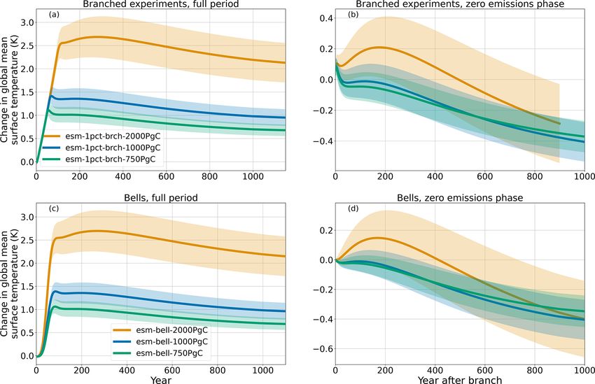
ments is illustrated in Fig. 3. It leads in abrupt-2xCO2 to
a radiative effect on the climate system, as a preindustrial
an unconstrained ECS of 2.74 ± 0.52 K (Table 2), reduced
level of CO2 is seen by the carbon cycle. In 1pctCO2-bgc,
to 2.52 ± 0.33 K with the constraints. Overall, the ECS is re-
only the carbon cycle is affected by CO2 , whereas a prein-
markably consistent in terms of average, standard deviation
dustrial CO2 is prescribed to the climate system. The outputs
and even skewness across the three abrupt experiments. This
of OSCAR v3.1 on these experiments are consistent with past
is due to the construction of OSCAR, with a prescribed log-
C4MIP results (Arora et al., 2013). The global mean surface
arithmic dependency of the radiative forcing of CO2 on its
temperature responds about linearly to the exponential in-
atmospheric concentration (Lurton et al., 2020). This ECS is
crease in CO2 because of the implemented logarithmic de-
lower than with the first approach because it includes sev-
pendency of the radiative forcing of CO2 on its atmospheric
eral Earth system feedbacks related to short-lived species
concentration. Carbon sinks rise in response to the increase
that are left free to change during the simulations, owing
in atmospheric CO2 , but the resulting warming dampens the
to the experimental protocol. In OSCAR, this is mostly ex-
sinks.
plained by an increase in the atmospheric load of tropo-
These three experiments can be used to calculate the
spheric aerosols (and ozone) caused by the endogenous emis-
carbon-concentration and carbon-climate feedback metrics,
sion of precursors through biomass burning. These feedbacks
respectively β and γ . These metrics, defined and used in for-
are also illustrated in Fig. 3. The RF resulting from the
mer C4MIP exercises (Friedlingstein et al., 2006; Arora et
prescribed change in atmospheric CO2 (7.42 W m−2 under
al., 2013, 2020), are a means to evaluate the model’s sen-
quadrupled CO2 ) is partially compensated for by short-lived
sitivities of the carbon stocks in the land and in the ocean
climate forcers. In the case of abrupt-4xCO2, the RF sums
to changes in atmospheric CO2 or GSAT. Table 3 summa-
up to 3.46 ± 0.25 W m−2 because of a cooling by scatter-
rizes these results. As explained by Arora et al. (2013), there
ing aerosols (−0.21±0.16 W m−2 ) and aerosol–cloud effects
are three methods to combine the three experiments to cal-
(−0.21 ± 0.15 W m−2 ), besides an additional warming from
culate the metrics: subtracting 1pctCO2-bgc from 1pctCO2-
absorbing aerosols (0.13 ± 0.08 W m−2 ). Finally, from Ta-
rad (denoted R-B, hereafter), subtracting 1pctCO2 from
https://doi.org/10.5194/gmd-16-1129-2023 Geosci. Model Dev., 16, 1129–1161, 2023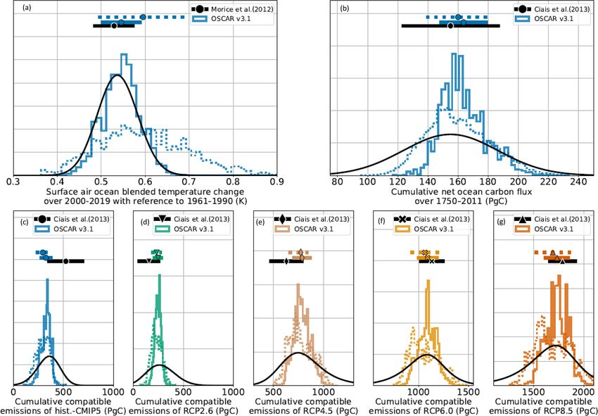
1136                                             Y. Quilcaille et al.: CMIP6 simulations with the compact Earth system model

Figure 3. Abrupt idealized experiments. In (a) the plain lines represent the average change in surface air temperature, and its ±1 standard
deviation ranges using shaded areas. Panels (b, c, d) show the contributions to the total RF at equilibrium. Individual contributions from
stratospheric O3 and deposition of black carbon (BC) on snow are inferior to 0.1 W m−2 in the abrupt-4xCO2 and have not been represented
for clarity. Panels (e, f, g) are the distributions of the ECS, calculated using equilibrium temperature, and thus include all the feedbacks of
OSCAR. The horizontal plain line is the ECS average and ±1 standard deviation range. These values with Pearson’s moment coefficient of
skewness are provided in the legend.

Table 3. Metrics of the carbon cycle (β and γ ) from the C4MIP experiments. Metrics are provided for OSCAR v3.1, constrained using obser-
vations and unconstrained. As explained by Arora et al. (2013), different values for the metrics are calculated depending on the combination
of experiments used: R stands for radiative (1pctCO2-rad), B for biogeochemical (1pctCO2-bgc) and F for full (1pctCO2). The change in
the land carbon stocks includes permafrost carbon. Results from CMIP5 and CMIP6 are provided by C4MIP (Arora et al., 2020).

    Time         Model                           Method β           β (PgC ppm−1 )           Method γ              γ (PgC K−1 )
                                                                  Land          Ocean                          Land             Ocean
                 OSCAR v3.1 constrained          R-B, B-F     1.26 ± 0.47     1.05 ± 0.03    R-B, R-F      −34.7 ± 18.9     −13.0 ± 0.7
                                                 R-F          1.21 ± 0.44     1.00 ± 0.06    B-F           −43.2 ± 23.8     −21.6 ± 6.3
    2 × CO2      OSCAR v3.1 unconstrained        R-B, B-F     1.14 ± 0.64     1.05 ± 0.03    R-B, R-F      −30.8 ± 20.5     −13.0 ± 0.7
                                                 R-F          1.10 ± 0.61     1.00 ± 0.05    B-F           −37.6 ± 26.4     −21.0 ± 5.7
                 CMIP5                           B-F          1.15 ± 0.63     0.95 ± 0.07    B-F           −37.0 ± 25.5      −9.4 ± 2.7
                 CMIP6                           B-F          1.22 ± 0.40     0.91 ± 0.09    B-F           −34.1 ± 38.4      −8.6 ± 2.9
                 OSCAR v3.1 constrained          R-B, B-F     1.06 ± 0.41     0.94 ± 0.03    R-B, R-F      −47.7 ± 23.8     −17.7 ± 1.3
                                                 R-F          0.95 ± 0.37     0.86 ± 0.08    B-F           −72.3 ± 37.4     −37.1 ± 13.6
    4 × CO2      OSCAR v3.1 unconstrained        R-B, B-F     0.96 ± 0.57     0.94 ± 0.03    R-B, R-F      −43.3 ± 25.5     −17.7 ± 1.3
                                                 R-F          0.87 ± 0.50     0.86 ± 0.07    B-F           −63.1 ± 41.5     −35.5 ± 12.4
                 CMIP5                           B-F          0.93 ± 0.49     0.82 ± 0.07    B-F           −57.9 ± 38.2     −17.3 ± 3.8
                 CMIP6                           B-F          0.97 ± 0.40     0.78 ± 0.07    B-F           −45.1 ± 50.6     −17.2 ± 4.9

Geosci. Model Dev., 16, 1129–1161, 2023                                                     https://doi.org/10.5194/gmd-16-1129-2023
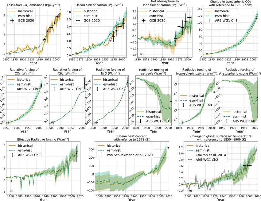
Y. Quilcaille et al.: CMIP6 simulations with the compact Earth system model                                                   1137

Figure 4. Experiments with 1 % increase in the atmospheric CO2 . The plain lines are the averages, and the shaded areas represent ±1
standard deviation ranges.

1pctCO2-bgc (B-F) and subtracting 1pctCO2 from 1pctCO2-             properly represent a saturation effect found in many ESMs.
rad (R-F). As shown in Table 3, methods R-B and B-F are             We note that in our assessment, the land includes permafrost
almost equivalent for β, while methods R-B and R-F are al-          carbon, which was not the case in CMIP5 assessment, but
most equivalent for γ . Although LUC affects these metrics          the permafrost is mostly sensitive to increase in temperatures
(Melnikova et al., 2022), these experiments are designed to         (i.e. it impacts γland but not βland ).
have a constant LUC.                                                   Overall, Table 3 shows that the unconstrained carbon cycle
   Table 3 shows that β under the R-F method is lower than          of OSCAR v3.1 is in line with CMIP exercises, particularly
the R-B and B-F because the non-linearity of the Earth sys-         CMIP5. Yet, the sensitivity of the oceanic carbon stock to in-
tem reduces the sensitivity of land and ocean carbon to atmo-       crease in GSAT remains too high. This bias in the ocean mod-
spheric CO2 . Similarly, γ under the R-B and R-F is higher          ule could be attributed to the stratification effect introduced
than under the B-F, but the non-linearity here is added to R-       in v2.2 (Gasser et al., 2017). In any case, this suggests that
B and B-F (Arora et al., 2013). Applying our observational          our carbon cycle may be too optimistic, which will clearly
constraints increases the absolute values of βland and γland of     appear in our emission-driven simulations.
OSCAR, but it does not affect the βocean and γocean signif-
icantly. The only exception is the γocean under the method          3.4   Reconstruction of the historical period
B-F. We note that the unconstrained OSCAR v3.1 is closer
to the CMIP5 exercises, be it at 2× or 4× CO2 . This re-            The concentration- and emission-driven historical experi-
sult can be explained with OSCAR v3.1 being calibrated on           ments (i.e. historical and esm-hist simulations, respectively)
CMIP5. However, the unconstrained βland is the only one to          were run with OSCAR. Their forcers differ only for CO2 : the
be closer to CMIP6 than to CMIP5. The cause of this dif-            atmospheric CO2 is prescribed in the former, whereas in the
ference in the βland remains unclear but may come from the          latter, fossil-fuel emissions are prescribed, and atmospheric
form of equation for the fertilization effect. The configura-       CO2 is fully interactive. In the concentration-driven histor-
tions of OSCAR are not only different parameters, but also          ical simulation, compatible fossil-fuel emissions are back-
different equations. Here, half of the configurations of OS-        calculated after the simulation (Jones et al., 2013; Gasser et
CAR follow a logarithmic formulation of the fertilization ef-       al., 2015). Altogether, these two simulations are relatively
fect (Gasser et al., 2017), which may not be convex enough to       close, as shown in Fig. 5, but with noticeable differences.

https://doi.org/10.5194/gmd-16-1129-2023                                               Geosci. Model Dev., 16, 1129–1161, 2023
1138                                            Y. Quilcaille et al.: CMIP6 simulations with the compact Earth system model

Figure 5. Emission- and concentration-driven historical scenarios. The plain lines are the averages, and the shaded areas represent ±1
standard deviation ranges. The fossil-fuel CO2 emissions for the concentration-driven historical simulation are the compatible emissions,
whereas those for the emissions-driven esm-hist are directly prescribed to OSCAR. Radiative forcings under esm-hist are not represented,
for they are too close to the concentration-driven historical simulation. Radiative forcings are with respect to 1750. The sources for the
observations are Friedlingstein et al. (2020) for GCB 2020, Hartmann et al. (2013) for AR5 WG1 Ch2, Ciais et al. (2013b) for AR5 WG1
Ch3 and Myhre et al. (2013) for AR5 WG1 Ch8. The 90 % ranges provided by AR5 are converted to the ±1 standard deviation ranges.

   Looking at the carbon cycle variables, we observe that up           of the two historical experiments is similar from the 1980s
to the 1940s, esm-histis was similar to the historical simula-         onward. For comparison, the estimate for this average net
tion in terms of fossil-fuel CO2 emissions, atmospheric CO2            land flux is 1.5 ± 1.1 PgC yr−1 over 2000–2009 (Friedling-
and both carbon sinks. For instance, the cumulative ocean              stein et al., 2020), while this flux calculated by OSCAR un-
sink over 1850–1940 is respectively 41 and 35 PgC in histor-           der historical and esm-hist simulations is 0.88 ± 0.48 and
ical and esm-hist simulations. The difference observed af-             0.85 ± 0.56 PgC yr−1 , respectively.
terwards can essentially be explained by the fact that the                Looking at the effective radiative forcings (ERFs), the
emission-driven simulation entirely misses the 1940s plateau           ERF of CO2 in the concentration-driven historical simula-
in atmospheric CO2 . Such a miss is typical of ESMs (Bastos            tion is directly deduced from the prescribed CO2 atmospheric
et al., 2016). For comparison after 1959, we use data from the         concentration (Meinshausen et al., 2017) but slightly higher
Global Carbon Budget (Friedlingstein et al., 2020), whose              by about 0.1 W m−2 than the central value from the 5th As-
assessment of ocean carbon sink is closer to our historical            sessment Report (AR5) (Myhre et al., 2013). The central
simulation than to our esm-hist simulation. The net carbon             value from AR5 (1.82 W m−2 ) is calculated with reference
flux from atmosphere to land (i.e. the aggregate of the land           to 1750 but becomes 1.66 W m−2 when calculated with refer-
sink, emissions from LUC and emissions from permafrost)                ence to 1850. This value increases to 1.70 W m−2 in CMIP6

Geosci. Model Dev., 16, 1129–1161, 2023                                                  https://doi.org/10.5194/gmd-16-1129-2023
Y. Quilcaille et al.: CMIP6 simulations with the compact Earth system model                                                    1139

data, mostly because of changes in the CO2 concentration in        3.5   Attributions
1850. With OSCAR and prescribed CO2 emissions, the at-
mospheric CO2 in esm-hist is higher than in the historical         DAMIP (Gillett et al., 2016) designed a number of experi-
simulation, and the ERF of CO2 is 0.2 W m−2 higher than            ments meant to attribute the observed climate change to an-
in the AR5. The ERF of other greenhouse gases is consis-           thropogenic and natural factors. Since OSCAR does not fea-
tent with Myhre et al. (2013). For most ERF components,            ture any internal variability, it cannot contribute to the “detec-
there is very little difference between historical and esm-hist.   tion” part of DAMIP. However, with more than 1000 Monte
OSCAR’s overall ability to simulate the RF of short-lived          Carlo elements, OSCAR is fully capable of carrying out the
species compares well with the IPCC AR5 values. Contribu-          “attribution” part. To achieve this attribution, DAMIP relies
tions to the warming from aerosols and ozone are consistent        on experiments that follow the historical one but in which
as well, although OSCAR tends to amplify these contribu-           only one forcing is turned on. Conversely, a number of other
tions. In 2011, IPCC AR5 estimates the RF from aerosols to         MIPs introduced attribution experiments in which all forc-
be −1.01 ± 0.37 W m−2 , while OSCAR calculates this to be          ings but the ones studied are turned on. However, neither of
−1.29 ± 0.52 W m−2 . Similarly, IPCC AR5 estimates the RF          these approaches explicitly considers the non-linearities of
from tropospheric ozone in 2011 to be 0.4 ± 0.2 W m−2 , and        the system. Other more robust methods of attribution to forc-
OSCAR estimates the RF to be 0.50±0.05 W m−2 . It may be           ings exist (Trudinger and Enting, 2005) and have been used
caused by overestimated biomass burning emissions, and this        with OSCAR in the past (Gasser, 2014; Li et al., 2016; Fu et
will be examined more in depth in a future analysis. Since         al., 2020; Ciais et al., 2013a). Here, we focus on results made
these biases were already evaluated in the description paper       possible with the CMIP6 experiments, which are presented in
of OSCAR (Gasser et al., 2017), it shows that our constrain-       Table 4.
ing does not markedly alter these aspects of the model. Addi-         In the historical experiment, we find a change in GSAT
tional constraining could be introduced for separate RF com-       of 0.98 ± 0.17 K in 2006–2015 with regard to 1850–1900,
ponents, although this would likely weaken the efficiency of       which is in line with observations because of our constrain-
other existing constraints.                                        ing setup (Sect. 2.3). Natural forcings caused only ∼ 0.03 K
   Looking at climate variables, the increase in GSAT in both      of this total, of which ∼ 0.02 and ∼ 0.01 were respectively
historical experiments is consistent with the Special Report       caused by solar and volcanic activity. Note that our volcano-
on Global Warming of 1.5C (IPCC, 2018) and with the his-           related forcing is defined against an average and constant vol-
torical reconstruction by Cowtan and Way (2013). During the        canic activity during the preindustrial period. This is why
choice of constraints (Sects. 2.3 and 3.1, Appendix A), we         the volcanic activity contributes only a positive ∼ 0.01 K
observed that constraints on temperatures impact our results       over the recent past where no major volcanic eruption hap-
much more than the other type of constraints. Even while           pened. In the IPCC terminology, our results lead to the con-
the set of constraints is expanded, constraints on temperature     clusion that it is extremely unlikely (i.e. likelihood < 1 %)
have a lasting influence over all outputs. The esm-hist simu-      that natural factors alone are causing the current observed
lation shows a higher GSAT and appears to be further away          climate change. This is of course consistent with the IPCC
from the observations. This is mostly the result of the higher     conclusions (Eyring et al., 2021; Gillett et al., 2021). Nev-
atmospheric CO2 seen earlier, and it suggests a different          ertheless, we note that our constraining reduces the uncer-
set of constraining weights could be used for the emission-        tainty range of all simulations, including those driven only
driven runs. We choose not to, for the sake of consistency.        by natural forcings. For the simulations under natural forc-
Comparing the effective radiative forcing (ERF) of OSCAR           ings, the range from the constrained OSCAR is smaller than
to the one of the IPCC AR5 (Myhre et al., 2013), we note           the ones from Gillett et al. (2021), which may suggest an
differences caused by volcanic eruptions. Beyond the update        over-constraining. It may be solved using different methods
of the time series of volcanic activity itself, OSCAR make         for constraining climate simulations (Nicholls et al., 2021b;
use of a warming efficacy of 0.6 for stratospheric volcanic        Williamson and Sansom, 2019).
aerosols (Gasser et al., 2017; Gregory et al., 2016). Never-          Since DAMIP did not include an experiment in which only
theless, IPCC AR5 estimates the ERF to be 2.3±1.0 W m−2 ,          natural forcings would be turned off, we cannot conclude as
while OSCAR calculates the ERF under historical and esm-           to the complementary probability of observed climate change
hist simulations to be 2.24 ± 0.48 and 2.34 ± 0.50 W m−2 ,         being caused only by anthropogenic factors (Gillett et al.,
respectively. Finally, the total ocean heat content is well re-    2021). Attribution to groups of anthropogenic forcings is
constructed, although the range of OSCAR is larger than the        possible, however. We find that 1.25 ± 0.11 K, about 128 %
observed one (von Schuckmann et al., 2020), suggesting this        of the recent warming, was caused by well-mixed green-
could also be considered a potential constraint for the model      house gases (WMGHGs), and −0.26 ± 0.22 K (−27 %) was
in future work.                                                    by near-term climate forcers (NTCFs). For comparison, the
                                                                   90 % confidence interval of CMIP6 over 2010–2019 instead
                                                                   of 2006–2015 is 1.16 to 1.95 K for WMGHGs and −0.73 to
                                                                   −0.14 K for NTCFs (Gillett et al., 2021). Another contribu-

https://doi.org/10.5194/gmd-16-1129-2023                                              Geosci. Model Dev., 16, 1129–1161, 2023
1140 Y. Quilcaille et al.: CMIP6 simulations with the compact Earth system model
Table 4. Attribution of historical and future climate change. These contributions come either from experiments in which only the concerned
forcing was prescribed (DAMIP) or from experiments in which it was removed (other MIPs). In either cases, non-linearities are ignored.
Experiments GSAT w.r.t. 1850–1900 (K) RF (W m−2 )
2006–2015 2091–2100 2006–2015 2091–2100 2006–2015 2091–2100
All forcings historical ssp245 0.98 ± 0.19 2.53 ± 0.25 2.07 ± 0.42 4.62 ± 0.29
WMGHGs1 hist-GHG ssp245-GHG 1.24 ± 0.12 2.67 ± 0.29 2.53 ± 0.13 4.73 ± 0.27
NTCFs2 hist-aer ssp245-aer −0.26 ± 0.22 −0.15 ± 0.12 −0.48 ± 0.36 −0.16 ± −0.12
id. historical – hist-piNTCF – −0.25 ± 0.21 – −0.46 ± 0.35 –
Natural forcings hist-nat ssp245-nat ∼ 0.03 ∼ 0.01 ∼ 0.09 ∼ 0.00
CO2 hist-CO2 ssp245-CO2 0.74 ± 0.07 2.03 ± 0.22 1.52 ± 0.09 3.70 ± 0.24
CO2 radiative effect only historical – hist-bgc – 0.75 ± 0.08 – 1.55 ± 0.04 –
CFCs and HCFCs1 historical – hist-1950HC – 0.13 ± 0.02 – 0.27 ± 0.03 –
Stratospheric O3 hist-stratO3 ssp245-stratO3 −0.03 ± 0.03 −0.02 ± 0.03 −0.07 ± 0.06 −0.02 ± 0.05
Aerosols historical – hist-piAer – −0.33 ± 0.20 – −0.63 ± 0.33 –
Solar activity hist-sol ssp245-sol ∼ 0.02 ∼ 0.01 ∼ 0.03 ∼ 0.02
Volcanic activity hist-volc ssp245-volc ∼ 0.01 ∼ −0.01 ∼ 0.06 ∼ −0.02
Land–sea change historical – hist-noLu – −0.03 ± 0.03 – −0.05 ± 0.05 –
1 In these experiments, because the atmospheric concentration of WMGHGs is prescribed, the indirect effects on tropospheric O (from CH ), stratospheric H O (from CH ) and
3 4 2 4
stratospheric O3 (from N2 O and halogenated compounds) are also included. 2 The effects listed in the previous note on WMGHGs are excluded from this experiment. Tropospheric O3
does vary but only because of the emission of ozone precursors and not because of varying atmospheric CH4 . Black carbon deposition on snow is also included in this experiment.
tion of −0.03±0.03 K (−3 %) is due to land-use change. We 3.6 Scenarios of climate change
highlight that observational constraints affect these contribu-
tions, as shown by Ribes et al. (2021), whose central esti- ScenarioMIP (O’Neill et al., 2016) chose eight particular
mate contributions over 2010–2019 are 116 % for WMGHGs Shared Socioeconomic Pathways (SSPs) taken from the SSP
and −32 % for NTCFs and land-use change. It follows that scenario database (Riahi et al., 2017) to cover a range of
the constrained results of OSCAR v3.1 are consistent with socio-economic assumptions and climate targets. After har-
Gillett et al. (2021) and Ribes et al. (2021). monization, these SSPs became the default CMIP6 scenar-
Considering the other experiments, we observe that the ios to be run by ESMs (Gidden et al., 2019). ScenarioMIP
DAMIP experiment (hist-aer) and the AerChemMIP one mostly required concentration-driven simulations up to the
(hist-piNTCF) led to very similar estimates of the contribu- year 2100 or 2300. In RCMIP, this was complemented by
tion of NTCFs (Table 4), which highlights that this part of our extending all scenarios up to 2500 and systematically run-
model behaves in a linear fashion. Going further in isolating ning emission-driven simulations in addition (Nicholls et al.,
individual forcings, we also estimate that CO2 caused 0.74 ± 2020). Figure 6 displays projections of key global variables
0.06 K, chlorofluorocarbons and hydro-chlorofluorocarbons of the Earth system following these scenarios, and Table 5
(i.e., CFCs and HCFCs) caused 0.13 ± 0.02 K, stratospheric focuses on projected GSAT changes.
O3 caused −0.03 ± 0.03 K and all aerosols together caused The climate target dimension of the SSP scenarios is de-
−0.33 ± 0.21 K (including direct and indirect effects). We fined similarly to the RCPs’ as the total RF targeted in
point out that details on CH4 , N2 O or tropospheric ozone 2100 (van Vuuren et al., 2011). Table 5 shows that this tar-
cannot be provided because of the lack of relevant CMIP6 geted RF is overall within the 1σ uncertainty range of all
experiments. our concentration-driven projections. In the cases with no-
The extent to which this attribution to specific forcings is table differences, such as ssp460, the actual RF reached by
comparable to existing studies remains unclear. One notable the reduced-complexity model MAGICC (IIASA, 2018a) for
limitation of OSCAR, in this respect, is that the model’s cli- this scenario is 5.29 W m−2 , which is then in the range of OS-
mate response is not forcing-dependent. The use of effective CAR. Although MAGICC was used for the design of these
radiative forcing is supposed to ensure that the temperature scenarios, this result demonstrates that we remain consistent
response to CO2 and non-CO2 forcings is similar, at least for with the intended RF of the scenarios. Emission-driven SSPs
the long-term steady state (Myhre et al., 2013). However, re- show lower RF than their concentration-driven counterparts,
cent work has pointed out that the response may strongly de- which can be attributed to a low bias in the atmospheric CO2
pend on the forcing agent (Marvel et al., 2016), thus casting that is especially visible in high-CO2 scenarios. This bias is
a degree of doubt on our attribution results. More work to in- a result of our constraining approach that favored configu-
tegrate such differentiated responses in reduced-complexity rations with strong CO2 fertilization (as also seen with the
models is warranted. C4MIP results, Sect. 3.3). Under high-CO2 scenarios, this
bias is likely worsened by our exclusion procedure during the
Geosci. Model Dev., 16, 1129–1161, 2023 https://doi.org/10.5194/gmd-16-1129-2023Y. Quilcaille et al.: CMIP6 simulations with the compact Earth system model 1141
Table 5. Projected atmospheric CO2 , RF and GSAT in SSPs. Concentration- and emission-driven experiments are shown and compared to
available CMIP6 projections. Values in bold are assumptions or inputs. Experiments whose name start with esm- are emission-driven; others
are concentration-driven. GSAT data from CMIP6 are provided as mean and standard deviation as well, with the number of models avail-
able in parentheses. Here, projections from OSCAR are constrained to observations, while CMIP6 results are raw, without any constraints
(Tokarska et al., 2020).
Experiments Models ERF (W m−2 ) GSAT w.r.t. 1850–1900 (K) CO2 (ppm)
2100 2041–2050 2091–2100 2291–2300 2491–2500 2100 2300
esm-ssp585 OSCAR 8.40 ± 0.57 2.02 ± 0.22 3.99 ± 0.40 6.31 ± 0.83 6.29 ± 0.88 1058 ± 63 1729 ± 148
esm-ssp585 CMIP6 2.41 ± 1.67 (3) 5.14 ± 3.92 (2)
ssp585 OSCAR 8.76 ± 0.50 2.04 ± 0.19 4.16 ± 0.38 7.05 ± 0.87 7.24 ± 0.93 1135 2162
ssp585 CMIP6 2.72 ± 1.51 (17) 6.19 ± 3.13 (17) 13.51 ± 5.87 (2) 1135 2162
esm-ssp370 OSCAR 7.04 ± 0.66 1.85 ± 0.25 3.32 ± 0.35 5.54 ± 0.74 5.56 ± 0.80 809 ± 47 1200 ± 109
ssp370 OSCAR 7.41 ± 0.58 1.87 ± 0.21 3.50 ± 0.32 6.24 ± 0.75 6.41 ± 0.81 867 1483
ssp370 CMIP6 2.51 ± 1.48 (18) 5.1 ± 2.84 (16) 867 1483
esm-ssp460 OSCAR 5.32 ± 0.50 1.80 ± 0.23 2.68 ± 0.30 3.43 ± 0.51 3.34 ± 0.55 629 ± 35 667 ± 49
ssp460 OSCAR 5.64 ± 0.40 1.82 ± 0.19 2.84 ± 0.27 3.91 ± 0.47 3.89 ± 0.50 668 769
ssp460 CMIP6 2.46 ± 1.28 (4) 4.24 ± 1.80 (4) 668 769
esm-ssp245 OSCAR 4.63 ± 0.43 1.72 ± 0.21 2.38 ± 0.28 2.59 ± 0.41 2.40 ± 0.42 578 ± 31 565 ± 35
ssp245 OSCAR 4.86 ± 0.31 1.75 ± 0.17 2.50 ± 0.25 2.92 ± 0.37 2.79 ± 0.37 603 621
ssp245 CMIP6 2.41 ± 1.33 (15) 3.63 ± 1.82 (15) 603 621
esm-ssp534-over OSCAR 2.93 ± 0.37 2.00 ± 0.22 1.73 ± 0.25 1.16 ± 0.23 1.02 ± 0.23 458 ± 23 374 ± 12
ssp534-over OSCAR 3.36 ± 0.27 2.04 ± 0.19 1.95 ± 0.22 1.40 ± 0.20 1.29 ± 0.19 497 398
ssp534-over CMIP6 2.88 ± 0.84 (6) 3.08 ± 1.06 (6) 1.85 ± 0.66 (2) 497 398
esm-ssp434 OSCAR 3.45 ± 0.40 1.64 ± 0.20 1.87 ± 0.24 1.51 ± 0.28 1.44 ± 0.29 451 ± 21 371 ± 15
ssp434 OSCAR 3.70 ± 0.31 1.65 ± 0.17 2.00 ± 0.21 1.73 ± 0.24 1.68 ± 0.25 473 392
ssp434 CMIP6 2.36 ± 1.1 (5) 3.23 ± 1.32 (5) 473 392
esm-ssp126 OSCAR 2.66 ± 0.29 1.54 ± 0.18 1.49 ± 0.21 1.17 ± 0.20 1.02 ± 0.20 439 ± 18 381 ± 11
ssp126 OSCAR 2.80 ± 0.20 1.58 ± 0.15 1.58 ± 0.17 1.31 ± 0.18 1.21 ± 0.18 446 396
ssp126 CMIP6 2.21 ± 1.1 (17) 2.38 ± 1.17 (17) 1.68 ± 0.7 (2) 446 396
esm-ssp119 OSCAR 2.0 ± 0.25 1.39 ± 0.17 1.15 ± 0.17 0.71 ± 0.15 0.61 ± 0.15 383 ± 12 334 ± 6
ssp119 OSCAR 2.14 ± 0.18 1.44 ± 0.14 1.24 ± 0.15 0.82 ± 0.13 0.74 ± 0.13 394 342
ssp119 CMIP6 2.36 ± 1.07 (6) 2.12 ± 0.92 (2) 394 342
post-processing, as very high CO2 tends to make the model degrees of freedom and likely release part of the constraint.
more unstable. The very low uncertainty range we obtain for When projecting temperature change in an emission-driven
projected atmospheric CO2 in emission-driven simulations mode, the uncertainty range is larger because of the addi-
is over-confident. We note that the constraints were derived tional uncertainty related to the biogeochemical cycles.
using concentration-driven simulations (that are the focus of The CMIP6 values are computed here from CMIP6 time
CMIP6), and so they may not apply properly to emission- series. However, some CMIP6 models exhibit higher warm-
driven simulations. ings than in previous assessments, and observations can be
The constraining approach contributes to having the used to constrain the future warming (Tokarska et al., 2020).
increases in GSAT for concentration-driven experiments Using their table S4, the warming in 2081–2100 with ref-
shown in Table 5 to be lower than the CMIP6 models we erence to 1995–2014 under SSP5-8.5 for the constrained
could compare our results to. The uncertainty range simu- CMIP6 models is 3.44 ± 0.67 and 3.11 ± 0.36 K for the con-
lated by OSCAR is also much lower, again owing to our strained OSCAR v3.1 model. For SSP1-2.6, the values are
constraining approach. With a relative uncertainty in GSAT respectively 0.94 ± 0.30 and 0.76 ± 0.17 K. Thus, the obser-
change in 2500 of ±13 % under the warmest scenario (SSP5- vational constraints that we have used contribute to explain-
8.5), these projections are likely to be over-constrained. This ing the differences to the raw CMIP6 data. Nevertheless, it
stems from our constraining of the climate response, as also remains that the climate module of OSCAR v3.1 could still
shown by the relatively small uncertainty range in ECS in the be improved.
idealized abrupt CO2 experiments. Further developing that
module by adding one or two key parameters (Geoffroy et
al., 2013a; Bloch-Johnson et al., 2015) would provide more
https://doi.org/10.5194/gmd-16-1129-2023 Geosci. Model Dev., 16, 1129–1161, 2023You can also read