Capillary fluctuations and energy dynamics for flow in porous media
←
→
Page content transcription
If your browser does not render page correctly, please read the page content below

Capillary fluctuations and energy dynamics for flow in porous media
                                                            James E. McClure,1 Steffen Berg,2 and Ryan T. Armstrong3
                                                            1) VirginiaPolytechnic Institute & State University, Blacksburg, Virginia
                                                            2) ShellGlobal Solutions International B.V. Grasweg 31, 1031HW Amsterdam, The Netherlands
                                                            3) University of New South Wales, Sydney

                                                            (*Electronic mail: mcclurej@vt.edu)
                                                            (Dated: 20 May 2021)
                                                            Capillary energy barriers have important consequences for immiscible fluid flow in porous media. We derive time-
                                                            and-space averaging theory to account for non-equilibrium behavior and understand the role of athermal capillary
                                                            fluctuations in the context of their relationship to larger scale phenomenological equations. The formulation resolves
arXiv:2012.09206v2 [physics.flu-dyn] 19 May 2021

                                                            several key challenges associated with two-fluid flow in porous media: (1) geometric and thermodynamic quantities are
                                                            constructed as smooth functions of time based on time-and space averages; (2) averaged thermodynamics are developed
                                                            for films; (3) multi-scale fluctuation terms are identified, which account for transient behaviours of interfaces and films
                                                            that occur due to pore-scale events; (4) geometric constraints are derived and imposed on the averaged thermodynamics;
                                                            (5) a new constitutive model is proposed for capillary pressure dynamics that includes contributions from films; and (6)
                                                            a time-and-space criterion for representative elementary volume (REV) is established based on capillary fluctuations.
                                                            Capillary fluctuations are assessed quantitatively based on pore-scale simulations and experimental core-flooding data.

                                                   I.   INTRODUCTION

                                                      The non-equilibrium response to fluid flow through porous
                                                   materials is inextricably linked to the length and time scales
                                                   for processes that occur within the solid micro-structure1–3 . It
                                                   is well known that fluid pressures fluctuate during immiscible
                                                   displacement as a consequence of pore-scale events4–6 . The
                                                   associated fluctuations are athermal and cooperative in nature
                                                   based on the fact that they arise due to the influence of cap-
                                                   illary forces7 . Theoretical treatment of these fluctuations is
                                                   of central importance to modeling due to the fact that ather-
                                                   mal fluctuations may not obey detailed balance8 . Since the re-
                                                   versibility of molecular interactions is central to the develop-
                                                   ment of Onsager’s non-equilibrium theory, the validity of phe-
                                                   nomenological equations depends on the properties of fluctu-
                                                   ations within the system9,10 . The validity of near-equilibrium
                                                   approximations and Onsager’s theory has been an important
                                                   assumption in many theoretical developments for fluid flow in
                                                   porous media11–15 .                                                 FIG. 1. Length and time scales for operative processes for multiphase
                                                      When multiple length scales are present within a system,         flows in porous media. Geometric effects directly link smaller-scale
                                                                                                                       phenomena with larger scale phenomena.
                                                   accompanying timescales will arise when considering the sys-
                                                   tem dynamics. The linkage between temporal, spatial and
                                                   energy scales is summarized in Fig. 1. Since information
                                                   cannot propagate instantaneously, processes that occur over         immiscible fluids in a geological setting, the timescale re-
                                                   small length scales will tend to be more rapid compared to          quired for diffusive processes to reach equilibrium is remark-
                                                   those that occur over larger length scales. Given a particular      ably slow; the timescale to reach equilibrium for Ostwald
                                                   length scale, the energy scale relates to the work needed to        ripening in CO2 -brine systems can be years18 . Within this
                                                   move matter and energy the requisite distance. The rate that        context, slow physics represent a critical consideration when
                                                   information propagates in the system is embedded in the phe-        applying near-equilibrium assumptions at macroscopic length
                                                   nomenological coefficients associated with particular physical      scales. The slow relaxation of diffusive systems explains the
                                                   processes. With respect to the validity of linear response the-     near-ubiquitous failure of Fick’s law in porous media19–22 .
                                                   ory, Onsager’s theory holds remarkably well in small systems,       While the timescale associated with capillary fluctuations is
                                                   implying that local near-equilibrium approximations are usu-        measured in seconds, the timescale to reach equilibrium can
                                                   ally reasonable16 . At small length scales, near-equilibrium        be hours to days in experimental systems23 . It is therefore
                                                   approximations are expected to fail only in extreme cases,          of great interest to develop non-equilibrium theory that does
                                                   such as in the immediate vicinity of shock waves17 . How-           not rely on macroscopic near-equilibrium assumptions. In this
                                                   ever, as the length scale associated with a process increases,      paper we develop such a theory.
                                                   so too does the required timescale to reach equilibrium. For           For multiphase flows in porous media, we identify three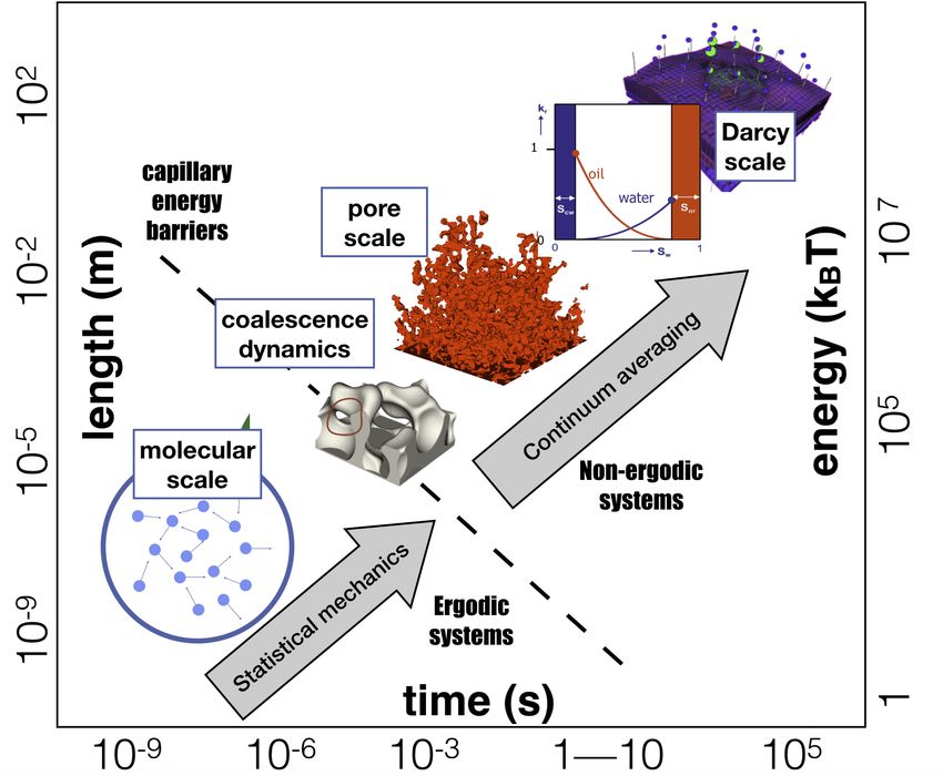
2

length scales of primary interest: (1) the interfacial length        curs at constant volume, such as capillary waves. To describe
scale associated with the width of the interface (10-50nm); (2)      these cases it is necessary to understand the non-equilibrium
the pore length scale associated with the solid micro-structure      response of the fluid pressures based on the capillary dynam-
(∼mm); and (3) the Darcy length scale associated with macro-         ics within the system.
scopic flow (cm - km). For each length scale, particular pro-            As fluids squeeze through the microstructure of complex
cesses of interest can be identified. At the interface length        materials subject to the influence of capillary forces, rapid
scale, film swelling effects can occur due to flow; coalescence      changes to the fluid configuration occur as the system jumps
events occur based on the merging of fluid regions, which            between metastable states. The displacement can be sub-
form loops or otherwise alter the fluid topology24 . Fluid sin-      divided into a sequence of isons and rheons4,5,43 . The as-
gularities result from the associated disruption to the inter-       sociated events are depicted in Fig. 2. Isons correspond to
face mean curvature25–38 . Snap-off events are also common           reversible displacement events where the fluid meniscus in-
in typical flow processes39 . At the pore length scale, Haines       vades a pore throat under quasi-static conditions, i.e. the fluid
jumps occur when fluid spontaneously fills regions of the            pressure difference is balanced by the capillary forces in the
the pore structure as fluids migrate between capillary energy        throat. The fluid pressure difference increases proportionate
barriers40 . These microscopic events are a primary source of        to the meniscus curvature as the interface is pushed into in-
non-equilibrium behavior, and are therefore a focus area when        creasingly narrow parts of the pore throat. When the menis-
considering the physical meaning of near equilibrium approx-         cus moves through the narrowest part of the pore neck, pore-
imations. The length scale of interest for flow processes is the     filling occurs spontaneously based on an event often known
Darcy scale, typically orders of magnitude larger than that of       as a Haines jump40 . As the meniscus curvature decreases,
the pore scale.                                                      the fluid pressure difference significantly exceeds the capil-
   In the following sections we provide a conceptual overview        lary pressure based on the interface curvature and fluid rapidly
of the basic physical considerations needed to model immis-          fills the pore. This irreversible event is known as a rheon.
cible displacement in porous media. Formal theoretical de-           Pore-filling events that transpire as Haines jumps can dissi-
velopment proceeds in six steps: (1) definition of the thermo-       pate a significant amount of energy1,2 . Furthermore, they oc-
dynamic system; (2) averaging in time-and-space; (3) rate of         cur very quickly (milliseconds to seconds) compared to typ-
external work in Darcy-scale systems; (4) analysis for fluc-         ical laboratory- and reservoir-scale process (hours to weeks).
tuations in solid wetting energy; and (5) derivation of geo-         Considering large systems, processes of interest involve very
metric constraints; (6) formulation of flux-force entropy and        large numbers of such events. Understanding their overall ef-
derivation of phenomenological equations for two-phase flow.         fect is of central importance to understanding transient effects
The derivation leads to explicit criteria for the validity of phe-   for multiphase flows in porous media.
nomenological equations based on the structure of capillary              The basis to consider multiphase flow in porous media as
fluctuations in the system. Using results from simulation and        a non-ergodic phenomenon is due to the rapid rate for lo-
experimental data, we directly evaluate the derived capillary        cal events at the pore-scale. In ergodic systems, energetic
fluctuation terms and consider the consequences for REV def-         micro-states are considered to be locally well-mixed due to
inition and the development of averaged descriptions for two-        thermal effects. Since the operative mixing mechanism is dif-
fluid flow in porous media.                                          fusive, the length scale for thermal mixing can be estimated
                                                                     based on the self-diffusion coefficient and timescale50 . When
                                                                     a mechanical event transfers energy more rapidly than diffu-
BACKGROUND                                                           sive thermal mechanisms, local symmetry breaking may oc-
                                                                     cur. Fig. 3 considers the length and time scale for seven
   At the pore scale, capillary forces are dominant and de-          Haines jump events observed during displacement in a micro-
termine how fluids are distributed within the solid micro-           fluidic system1 . The distance traveled by the fluid meniscus
structure. Capillary pressure accounts for the contribution          is plotted versus the elapsed time for each event. This can be
of surface forces created by the surface energy and meniscus         compared to the length scale for diffusive mixing during the
curvature41 . The Young-Laplace equation relates the pressure        elapsed time is ∆t, given by
difference between the adjoining fluids and the capillary pres-                                      √
sure given by the product of the interfacial tension γ and mean                                ∆x = D∆t ,                          (2)
curvature,
                                                                     where D = 2.299 × 10⁻⁵ cm2 / sec is the self-diffusion coef-
                                1       1                          ficient for water. We classify a phenomenon as ergodic if the
                  pn − pw = γwn       +        ,            (1)      distance traveled over a particular time interval is smaller than
                                   R1 R2
                                                                     the diffusive length scale. A phenomenon is classified as non-
where R1 and R2 are the principal curvature radii at points          ergodic if the distance traveled during an interval of time ex-
on the fluid meniscus. The Laplace equation holds only at            ceeds this distance. Fig. 3 clearly shows that Haines jumps be-
mechanical equilibrium, and does not account for dynamic             gin in the ergodic region but cross into the non-ergodic regime
processes that involve moving interfaces. This necessarily           as capillary energy is converted into kinetic energy. Over the
includes any process where the fluid volumes change, since           timescale for a Haines jump, the length scale for thermal mix-
these changes can only occur based on movement of the in-            ing is an order of magnitude smaller than the characteristic
terface. Situations also arise where interface movement oc-          length scale for the event. The system can therefore be con-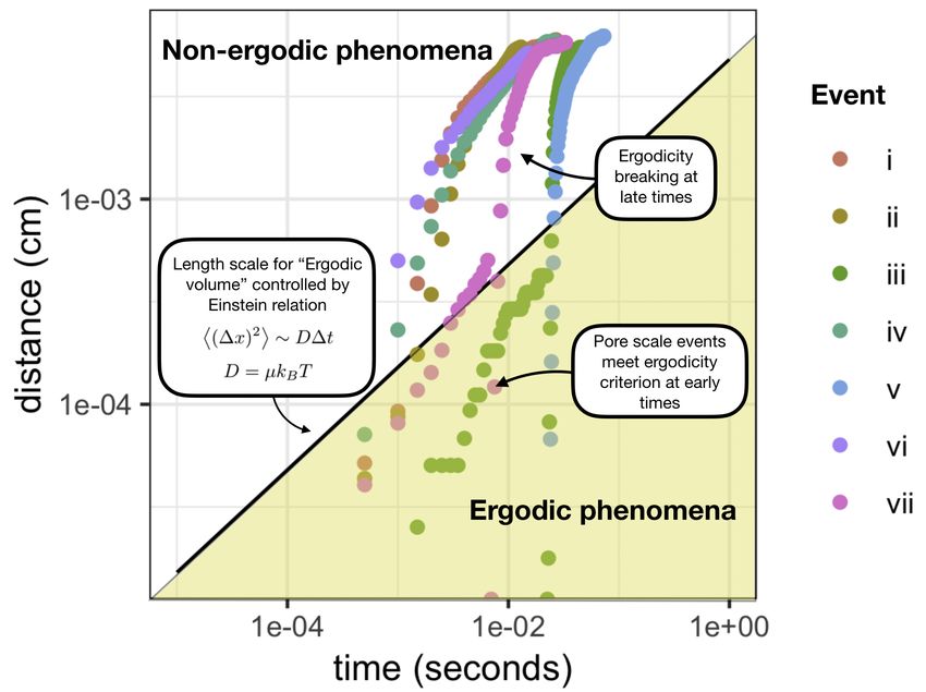
3

FIG. 2. Pore-scale displacement events can be separated into reversible events called isons and irreversible rheons (a) Isons correspond to
reversible displacement as the capillary pressure increases, forcing the fluid meniscus into narrower pore throats. When the meniscus passes
through the narrowest part of the pore-throat, energy is released during the ensuing pore-filling event. A rapid drop in capillary pressure occurs
as the meniscus curvature decreases, which corresponds to a rheon. Fluid then spontaneously fills the pore until the local capillary pressure is
again balanced by the fluid pressure difference; (b) identification of ison, rheon and sub-ison events from experimental data.

                                                     √
sidered to be thermally well-mixed at the scale of D∆t, but                rate of energy dissipated within the system is thereby embed-
not at the scale of a Haines jump.                                         ded in kri .
   At the Darcy scale, energy that is dissipated from pore-scale              Pressure-volume work occurs when one fluid displaces an-
events can be estimated from basic concepts of work and en-                other. Considering a wetting and non-wetting fluid with pres-
ergy. A typical experiment can be treated as a system where                sure pw and pn , this contribution to the external work is given
external work is performed in two primary ways. First is the               by
work associated with fluid flow. The volumetric flow rate is
Qi for each fluid i ∈ {w, n} results due to external work per-                                  ∂Wext              ∂Vw
                                                                                                      = (pw − pn )     .                      (5)
formed on the system by some external potential Φi , e.g. due                                    ∂t                 ∂t
to an external pressure gradient or body force. Since work
                                                                           External work performed on the system is transferred to the
is defined as the applied force multiplied by the distance, the
                                                                           internal energy modes, which include contributions to the in-
total rate of work is
                                                                           ternal thermal energy from dissipated heat. Changes to the
                  dWdarcy                                                  surface energy account for a significant part of the external
                          = ∑ ∆Φi Qi · nb ,                        (3)     pressure-volume work. If the solid material is water-wet,
                    dt     i∈{w,n}
                                                                           the change in surface energy is proportional to the change
                 (in)     (out)                                            in surface area based on the interfacial tension γwn . Mor-
where ∆Φi = Φi − Φi          is the potential difference between
                                                                           row therefore defined the displacement efficiency as the frac-
the inlet and the outlet and nb is the boundary normal vector.
                                                                           tion of pressure-volume work that is converted to surface
This expression is is directly implied from the definition of
                                                                           energy5 . Seth and Morrow showed that the efficiency for a pri-
mechanical work. The boundary terms can also be obtained
                                                                           mary drainage varies from 10–95% depending on the material
by applying the divergence theorem in consideration of the
                                                                           type42 . The dissipated energy can also be estimated from the
internal stresses43 . Conceptually, the work due to Darcy flow
                                                                           mechanistic picture illustrated in Fig. 2. The pressure-volume
occurs in a steady-state system, meaning that there are no net
                                                                           work associated with an initial ison can be considered to be re-
changes to the internal energy, with each fluid forming static
                                                                           versible based on the fact that the displacement is quasi-static.
connected pathways through the sample that allow flow to oc-
                                                                           Since a rheon is spontaneous, the work associated with the
cur. The conventional relative permeability relationship pre-
                                                                           ensuing sub-ison accounts for the dissipated energy after any
dicts the flux per area as
                                                                           surface energy changes generated by the event has been sub-
                                  kri                                      tracted. With energy input into the system given by Eqs. 4 and
                        qi = −        K · ∇Φi ,                    (4)     5, the internal energy dynamics of the system can be treated
                                  µi
                                                                           based on conservation of energy.
where qi = Qi /A, kri is the relative permeability, µi is the dy-             Models for capillary pressure dynamics have been previ-
namic viscosity and K is the permeability tensor for the mate-             ously developed to account for the macroscopic behaviour
rial. This can be combined with Eq. 3 to approximate the rate              during displacement. The first such models were developed
of work based on an applied external potential gradient. The               using concepts of work and energy5 . Subsequent models in-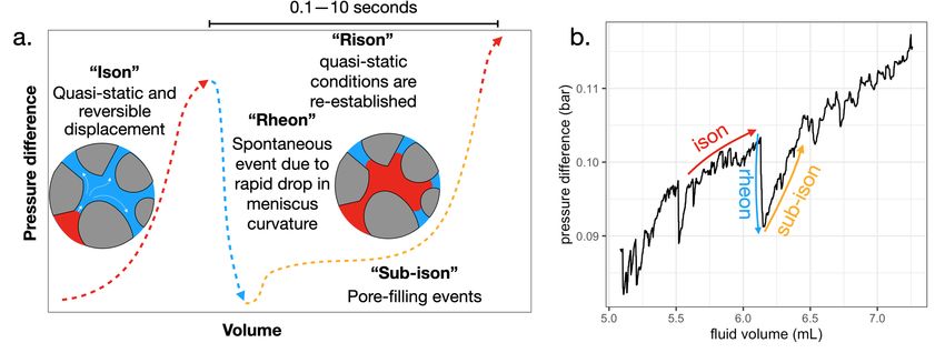
4

                                                                         models such as the conventional relative permeability rela-
                                                                         tionship. A new expression for the dynamic capillary pressure
                                                                         is also derived, which directly includes effects due to fluctua-
                                                                         tions. Capillary fluctuations are then directly evaluated based
                                                                         on pore-scale simulations and experimental data.

                                                                         II.    THEORETICAL APPROACH

                                                                            In the following sections we present the theoretical ap-
                                                                         proach used to derive constitutive models for immiscible fluid
                                                                         flow through porous media. Our approach relies on averaging
                                                                         in both time and space, which is distinct from previously de-
                                                                         veloped models. Capillary fluctuation terms are included ex-
                                                                         plicitly, and special treatment is needed to develop a flux-force
                                                                         entropy inequality that accounts for the associated energy dy-
                                                                         namics. The flux-force form of the entropy inequality can be
FIG. 3. The length scale for mixing can be estimated from the mean-      exploited to derive standard expressions for relative perme-
squared distance for self-diffusion over a given length of time. Pore-
                                                                         ability as well as a dynamic capillary pressure relationship to
scale events such as Haines jumps are associated with ergodicity
breaking due to the rapid dynamics caused by the transfer of surface
                                                                         describe unsteady displacement. The theoretical approach is
energy to other internal energy modes. Colored dots depict the ob-       organized into six steps:
served trajectory for seven different Haines jumps in a microfluidic
system.                                                                        1. Thermodynamic description – variables required to
                                                                                  formulate a classical thermodynamic description at a
                                                                                  scale where the behavior is ergodic, including effects
                                                                                  due to fluid phases, interfaces and films;
corporated concepts of non-equilibrium thermodynamics11,15
and kinematics13,44 . Previously developed models fail to deal                 2. Averages in space and time – averaging is applied to
with the challenges associated with the non-smooth response                       develop thermodynamic forms that hold at larger length
of the fluid pressure and interfacial curvature. This criti-                      and time scales. Fluctuation terms arise as a conse-
cal challenge is associated with changes to the fluid topol-                      quence of averaging in both space and time.
ogy, which necessarily cause a discontinuity in the interfa-
cial curvature24,30,37 . The apparent geometric discontinuity                  3. Rate of work and entropy inequality – an entropy in-
links to questions about whether or not multi-fluid systems                       equality is developed by defining the rate of external
can be considered to be in a near-equilibrium state. Bear                         work associated with fluid flow;
& Nitao argue that while relatively simple macroscopic ther-
modynamic equations of state must exist at equilibrium due                     4. Surface wetting fluctuations – analysis is performed
to the Gibbs phase rule, these relations will break down un-                      to interpret the surface wetting fluctuation term;
der non-equilibrium conditions if the mean-square deviation
                                                                               5. Geometric constraints – a geometric constraint is
is too large14 . For systems with slow physics, near equilib-
                                                                                  needed to relate the time derivative for the interfacial
rium conditions can break down as the length scale for the
                                                                                  area to the time derivative for the fluid volume frac-
REV increases due to the larger timescale required for mixing
                                                                                  tional. A relationship between partial derivatives for
to occur. We argue that the breakdown of near-equilibrium
                                                                                  geometric quantities is derived;
behavior will occur at large length scales based on the ar-
gument summarized in Fig. 3. Near-equilibrium
                                            √       conditions                 6. Flux-force form of entropy inequality – all results are
should hold at spatial scales smaller than D∆t, with ∆t be-                       combined to form a flux-force form of the entropy in-
ing the timescale for pore-scale events. Averaging in time-                       equality. A REV constraint is derived for the fluctu-
and-space provides a way to upscale the formulation to larger                     ations. Provided the constraint is met, standard rela-
length and time scales based on a near-equilibrium approxi-                       tive permeability relationships are obtained as well as
mation at a small scale. Upscaling is then performed based                        a form to approximate the capillary pressure dynamics
on integrals, which do not require any near-equilibrium ap-                       during unsteady displacement.
proximation at at the larger scale. In this work, we consider
how multi-scale effects influence the transient capillary pres-          By explicitly considering the contribution from fluctuations
sure behavior and consider consequences for the rate of en-              in the flux-force form of the entropy inequality, conditions for
ergy dissipation. Multi-scale fluctuation terms are identified           the validity of Darcy-scale phenomenological equations can
explicitly, which can be directly evaluated and compared to              be developed explicitly. The derived condition is a constraint
other energy dynamics within the system. Conditions derived              on the representative elementary volume (REV) for the sys-
based on these fluctuation terms clearly demonstrate when                tem, which considers both spatial and temporal aspects. The
Onsager theory can be applied to derive phenomenological                 theory does not rely on the assumption of detailed balance at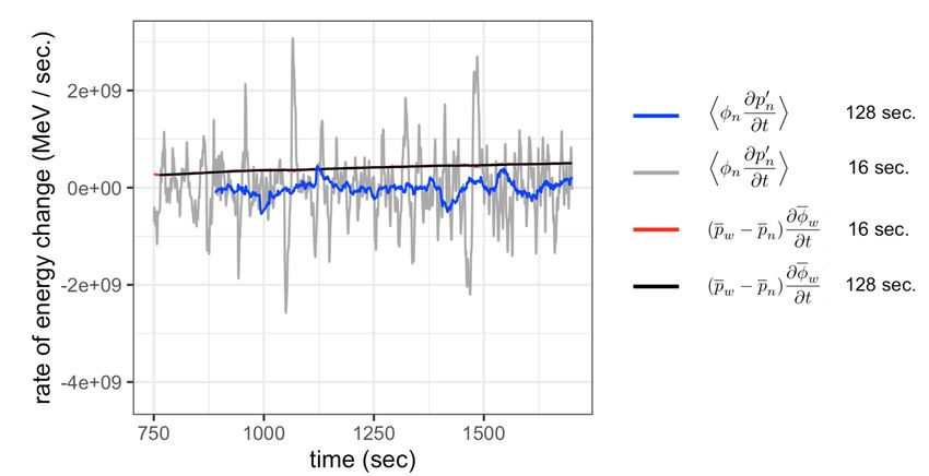
5

the macroscopic scale, as ergodic conditions are assumed to           In a strongly wetted system, the solid surface is coated ev-
hold only at small length scales. The derived REV condition is        erywhere by a thin film of fluid w. This means that fluid n
a constraint that fluctuations must obey to derive phenomeno-         interacts with w everywhere along its boundary, described by
logical equations that provide a valid representation for the         the surface energy γwn . If the system is not strongly wetted by
entropy production in the system. Experimental data is then           w, the formulation can still be used based on the fact that any
used to assess the role of capillary fluctuations in the context      excess energy due to interactions between the fluids and the
of the theory.                                                        solid will be accounted for by local variations in γs along the
                                                                      solid. The complexity of the fluid-solid interactions is there-
                                                                      fore embedded within the associated energy term, γs As . In our
A.   Thermodynamic Description                                        approach, we do not treat the solid as being in contact with a
                                                                      particular fluid. Instead we consider the situation where the
   Thermodynamics provides a mechanism to link flow pro-              associated interfacial energy γs and film thickness hs can vary
cesses with conservation of energy. For non-equilibrium sys-          along the solid. The formulation presupposes that films coat
tems, this is accomplished by deriving an expression for the          the solid surface everywhere, with the understanding that if
entropy production, which can then be exploited to derive phe-        the film thickness hs = 0 locally on portions of the solid sur-
nomenological equations for particular processes10 . At the           face, this will be equivalent to treating films as covering only
practical level, thermodynamics is a multi-scale book-keeping         part of the solid surface. The disjoining pressure is defined as
system to keep track of how energy is distributed within a sys-
tem. The thermodynamics of heterogeneous systems are typi-                                1  ∂U
                                                                                 Πs ≡ −                                             (8)
cally treated by dividing the system into sub-regions based on                            As ∂ hs S,Vw ,Vn ,An ,As ,Nak ,Nbk ,Nsk
the system composition12,45,46 . In addition to the entropy S
we consider the extensive variables to be                             The energy due to fluid-solid interactions is therefore lumped
                                                                      into two terms, one associated with the interfacial energy and
     • Vi – fluid volume for i ∈ {w, n}                               a second due to the disjoining pressure and film contributions.
                                                                      Variations in γs and hs along the surface of the solid occur
     • An – surface area for fluid n                                  due to the interaction between the fluid and solid material,
                                                                      including the effects of roughness and chemical heterogeneity.
     • As – surface area for the solid material
                                                                         The terms that account for capillary fluctuations are ne-
     • hs – film thickness along the solid material                   glected in conventional non-equilibrium thermodynamics;
                                                                      these appear only when time-averages are introduced. When
     • Nik – number of molecules of type k within any region          considering flow processes that occur over long periods of
       i ∈ {w, n, s}                                                  time, it is easy to overlook fast dynamics. Haines jumps are
                                                                      one such category of event, with dynamics that typically occur
For simplicity energy associated with the solid is omitted,           over a duration of milliseconds to seconds2,47,48 . Topological
such as effects associated with deformation. Considering              changes such as droplet coalescence also dissipate energy, oc-
solid that does not deform, the surface area bounding the wet-        curring even more rapidly and contributing to pressure fluctu-
ting fluid Aw is omitted based on the fact that only two of           ations. While both classes of event are common for flows in
{An , Aw , As } are independent. The internal energy is given as      porous media, the associated energy dissipation has not been
a function of the independent extensive quantities                    properly included in thermodynamic models. In the following
                                                                      sections, we demonstrate that pressure fluctuations represent
          U = U(S,Vw ,Vn , An , As , hs , Nak , Nbk , Nsk ) .   (6)   an essential contribution to the energy dynamics for two-fluid
                                                                      flow in porous media.
The Euler equation for the internal energy of the system is
then written as

       U = T S − pwVw − pnVn + γwn An + γs As − Πs hs As              B.   Thermodynamic Averages in Space and Time
           +µak Nak + µbk Nbk + µsk Nsk ,                       (7)
                                                                         The use of time averaging to study non-equilibrium behav-
where the intensive measures are                                      ior for two-fluid flow in porous media was first treated by
                                                                      Aryana and Kovscek49 . While these authors demonstrated
     • pi – fluid pressure for i ∈ {w, n}                             that the conventional Buckley-Leverett model could be de-
     • γwn – surface energy for fluid-fluid interface                 rived based on this approach (as well as extended models), as-
                                                                      pects pertaining to the non-equlibrium thermodynamics were
     • γs – surface energy for the solid material                     not considered. Here we develop this theory explicitly. Aver-
                                                                      ages are constructed with the time-and-space averaging oper-
     • Πs – disjoining pressure along the solid material              ator, defined as

     • µik – chemical potential for molecule k within any re-                                     1
                                                                                                      Z Z
       gion i ∈ {w, n, s}                                                                 f ≡                  f dV dt ,            (9)
                                                                                                 λV     Λ Ω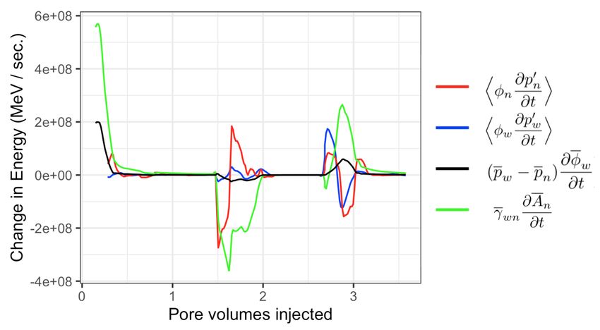
6

where Λ is a region of time with duration λ and Ω is a spa-                 The time derivative for the internal energy includes contribu-
tial averaging region50 . V is the volume associated with ther-             tions from the time derivatives of the averages of the extensive
modynamic measurements which can be estimated from the                      measures as well as fluctuation terms that arise due to the mi-
length scale given in Eq. 2. For example, if the fluid pres-                croscopic deviations in the intensive quantities
sure is measured with a transducer, V can be thought of as
the volume of fluid that is in local equilibrium with the mea-                 ∂U    ∂S       ∂V w        ∂V n         ∂ N ik        ∂ An
                                                                                  =T     − pw        − pn       + µ ik        + γ wn
sured value as a consequence of local mixing due to motion of                  ∂t    ∂t        ∂t          ∂t           ∂t            ∂t
molecules in the immediate vicinity. The total volume of the                                      ∂ As         ∂ hs    D   ∂T   0 E
spatial averaging region Ω is V > V . Dividing Eq. 7 by V                          + γ s − Πs hs        − Πs As      − S
                                                                                                    ∂t           ∂t           ∂t
leads to a representation of the internal energy on a per-unit-                      D ∂ p0 E D ∂ p0 E D ∂ µ 0 E
volume basis. Since a point in space may be within one fluid                       + Vw w + Vn n − Nik ik
or the other, we define the indicator function                                            ∂t             ∂t              ∂t
                                                                                     D ∂ γ0 E D ∂ γ0 E D                 ∂ Π0s E
                                                                                            wn              s

                               1 if x ∈ Ωi                                         − An           − As         + As hs             ,     (15)
                   φi (x) =                                (10)                           ∂t             ∂t               ∂t
                               0 otherwise
                                                                            where a sum is implied for all chemical potential terms. The
where i ∈ {w, n} to denote the region of space occupied by                  multi-scale fluctuation terms account for transient effects and
each fluid, Ωi . Integrating φi over any region will therefore              heterogeneity associated with the thermodynamic behaviour:
return the volume of the associated fluid within that region.
                                                                                      ∂ p0
                                                                                  D         E
   Statistical definitions for thermodynamic quantities rely on                 • Vi ∂t i – fluid pressure fluctuations, e.g. due to the
the ergodic hypothesis such that ensemble averages are the
                                                                                  transient effect of changing capillary forces on the fluid
same as averages in space or time. The basis for this assump-
                                                                                  pressure during flow;
tion is that the energy micro-states are locally well-mixed, i.e.
that the molecules in the system interact and exchange energy                     D
                                                                                       ∂ γ0
                                                                                              E
on a timescale that is sufficiently fast relative to the size of the            • An ∂twn – fluctuations to the fluid-fluid interfacial
system considered. Within this context Eq. 7 holds in the limit                   tension, e.g. due to different surface tension along the
of infinite time and non-equilibrium expressions must be de-                      fluid-fluid interface, which may arise if surfactants are
veloped to study time-dependent processes. In the context of                      present;
ergodic theory, the averaging operator given by Eq. 9 explic-
                                                                                          0
                                                                                  D         E
itly mixes information in space and time to generate averages.                  • As ∂∂tγs – fluctuations to the fluid-solid surface energy,
Non-ergodic effects can be accounted for in the averaged sys-                     e.g. which occur due to movement of the contact line
tem provided that Λ and Ω are chosen appropriately. Averages                      and complex fluid-solid interactions that occur due to
of the extensive quantities are simple averages so that these                     surface heterogeneity;
quantities retain their basic meaning
                                                                                              0
                                                                                  D             E
      S≡ S ,       V i ≡ V φ i = V φi ,            N ik ≡ Nik ,                 • As hs ∂∂tΠs – fluctuations to the disjoining pressure of
                    Ai ≡ Ai ,          hs ≡ hs ,                     (11)         films on the solid surface, e.g. which can occur due to
                                                                                  localized film swelling;
The intensive measures are then defined to maintain scale-
consistency with Eq. 7                                                            D
                                                                                        ∂ µ0
                                                                                              E
                                                                                • Nik ∂tik – fluctuations to chemical potential, which
              TS                    pi φi              µik Nik                    arise due to mass diffusion.
       T≡        ,       pi ≡             ,   µ ik ≡           ,
              S                      φi                 Nik
                                                                               There is a direct link between the pressure fluctuation de-
                                                                            fined in Eq. 15, and rugged energy landscapes depicted in
                       γi A i                 Πs As hs                      Fig. 2. Pressure fluctuation terms contribute to the non-
               γi ≡           ,      Πs ≡              .             (12)
                        Ai                     As hs                        equilibrium description based on pore-scale events that tran-
                                                                            spire within the averaging window defined by Λ and Ω. The
The internal energy in the averaged thermodynamic model                     reversible work associated with an ison is captured based on
will then be given by                                                       the product of the fluid pressure difference and rate of vol-
      U = T S − pwV w − pnV n + γ wn An + γ s As − Πs As hs                 ume change, as in standard non-equilibrium thermodynam-
                                                                            ics. During a strictly quasi-static displacement, the rate of
          +µ ak N ak + µ bk N bk + µ sk N sk .              (13)
                                                                            change for the microscopic pressure pi should closely corre-
   In a non-equilibrium system, deviations of the intensive                 spond with the average fluid pressure pi . On the other hand, if
quantities contribute to the energy dynamics50 . The deviation              we consider a rheon to be a rapid pressure change at constant
terms are defined as the difference between the microscopic                 volume, then pi must deviate significantly from pi over the
value and the averaged value                                                duration of the event. Therefore, if there are rheons occuring
                                                                            within Ω during the time interval Λ then the associated fluctu-
       T0 ≡ T −T ,       p0i ≡ pi − pi ,       µik0 ≡ µik − µ ik ,          ation terms are expected to have a significant effect. This will
                 γi0 ≡ γi − γ i ,     Π0s ≡ Πs − Πs .                (14)   be treated in more detail in sections to follow.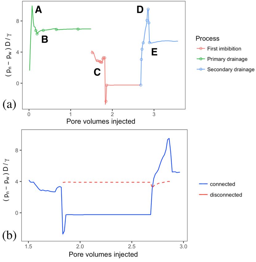
7

C.    Rate of work and entropy inequality                            where L is the distance between the sample inlet and outlet
                                                                     and the time-average for the fluid volume fraction is
  The change to the internal energy of the system is deter-
                                                                                               Vi
mined based on the rate of work done on the system and the                              φi =        for i ∈ {w, n} .             (18)
heat added                                                                                     V
                                                                     In the context of Fig. 2, specific terms appear that correspond
                          ∂U   ∂W ∂ Q
                             =     +    .                    (16)    with the reversible pressure-volume work associated with an
                          ∂t    ∂t   ∂t                              ison and the spontaneous rheons. Note that the average pres-
The instantaneous rate of work is given by the sum of Eqs. 3         sure will behave as a smooth function of time, meaning that
and 5, the latter being already built into the thermodynamics.       the “rugged" parts of the energy landscape can be fully trans-
For the data considered in this work, which correspond to im-        ferred to the fluctuation terms if Λ is large enough. Three
miscible two-fluid flow in strongly water-wet systems, several       fluctuation terms are retained, the first associated with cap-
assumptions can be made to simplify the form of Eq. 15:              illary fluctuations in the fluid pressures. The second is due
                                                                     to wetting fluctuations that are attributed to the movement of
     1. the system temperature is uniform and no heat is added       the contact line during fluid displacement, which appears due
        to the system, which is justified by the large heat capac-   to the time derivative for the deviation of the solid interac-
        ity for the system,                                          tion energy γs0 . Intuitively, the fluid-solid interaction energy
                                                                     changes when the contact line moves. Finally, the effects of
                    D ∂T0 E                  ∂Q                      film swelling contribute based on the fluctuation of the dis-
              T =T → S      =0,                 =0;                  joining pressure, which will change based on changes to the
                       ∂t                    ∂t
                                                                     film thickness. This contribution is important primarily when
     2. the fluid-fluid interfacial tension is constant every-       the wetting fluid is poorly connected, in which case films that
        where:                                                       coat the solid surface provide a primary flow pathway for that
                                                                     fluid. To obtain a more useful form of the entropy inequality,
                              D ∂ γ0 E                               a flux-force form must be obtained9 . In the following sec-
                  γwn = γ wn → An wn = 0 ;                           tions we demonstrate how this can be accomplished for sys-
                                  ∂t
                                                                     tems where the fluctuation terms play a significant role.
     3. the solid does not change shape, meaning that
                                                                     D.   Fluctuations and solid wetting energy
                   ∂ As             ∂V w    ∂V n
                        =0,              =−      ;
                    ∂t               ∂t      ∂t
                                                                        The model considered here is developed for strongly water-
                                                                     wet systems where the solid is coated everywhere by a thin
     4. compositional effects can be ignored
                                                                     water film. This means that the boundary of the non-wetting
                                     D ∂ µ0 E                        fluid touches water everywhere, and the surface energy is pro-
                       ∂ N ik
                µ ik          =0,     Nik ik = 0 .                   portional to the total boundary surface area An . This simplifies
                        ∂t               ∂t                          the geometric analysis presented in the next section. For the
                                                                     situations considered here, where the surface wetting proper-
Subject to these assumptions and using Eq. 16 to replace the         ties are homogeneous and do not change with time, the surface
change to the internal energy with the rate of external work         wetting fluctuation is zero,
done on the system, Eq. 15 can be simplified and rearranged
to obtain an entropy inequality                                                         ∂ γs0      D ∂ γ0 E
                                                                                              = 0 → As s = 0                     (19)
               (                                                                        ∂t            ∂t
      ∂S     1     h                    i
          =      L ∇Φw · Qw + ∇Φn · Qn                               In many situations the surface wetting properties will be het-
      ∂t     T |            {z          }                            erogeneous, with the local wetting energy varying based on
                     work of fluid flow                              chemical properties and roughness of the solid. In these more
                h          ∂φ       D ∂ p0      ∂ p0 E i             general conditions, all of the the solid surface energy contri-
            +V (pw − pn ) w − φw w + φn n                            butions are embedded into a single term. This term can also
                  |     {z ∂t } |       ∂t {z    ∂t }
                                                                     account for situations where the solid is not strongly wetted
                        ison                rheon                    by one fluid. In this case only part of the solid is in contact
                      ∂ An D ∂ γs0 E                                 with water, with associated surface area Aws . The rest of the
             − γ wn        + As
                 | ∂t {z         ∂t }                                solid contacts the non-wetting fluid, with Ans = As + Aws . In
               change in surface energy                              this situation the fluctuation term can be subdivided into dis-
                                          )                          tinct regions of water and non-wetting fluid contact the grain
                     ∂ hs D       ∂ Π0s E                            surface.
             + As Πs      − As hs           ≥0,              (17)
                      ∂t {z        ∂t }                                          D ∂ γ0 E D ∂ γ0 E D            ∂ γ0 E
                                                                                  As s = Ans s + Aws s = 0
               |
                     film swelling                                                                                              (20)
                                                                                      ∂t            ∂t           ∂t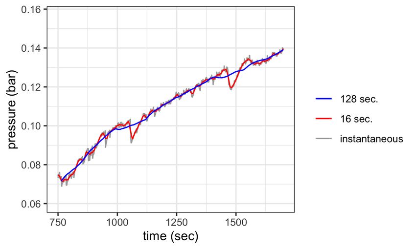
8

If the solid surface energy is constant over each region with       a non-dimensional relationship developed based on invariant
γs = γ ws everywhere on Aws and γs = γ ns everywhere on Ans ,       measures of integral geometry24 . Here we apply this relation-
then                                                                ship to the time-and-space averaged geometric measures
                      γs As       γ ns Ans + γ ws Aws
               γs =           =                       .     (21)                           f (φ n ,W n , X n ) = 0 .               (25)
                       As                  As
In this case fluctuations of the solid surface energy are deter-    The non-dimensional measures are defined as
mined by movement of the contact line, which changes the
                                                                                                 2
surface areas. Since γ ns , γ ws and As are constant with respect                               An              χ n An
to time,                                                                             Wn =           ,    Xn =          2
                                                                                                                           .       (26)
                                                                                               H nV               Hn
              ∂ γs   1  ∂ Ans         ∂ Aws
                   =    γ ns    + γ ws         .            (22)    where An is the time average for the surface area of the non-
               ∂t    As      ∂t          ∂t
                                                                    wetting fluid boundary, H n is the time average of integral
Since the total solid surface area is constant                      mean curvature, and χ n is the time average for the Euler char-
                                                                    acteristic. Even though the instantaneously measured χn is
                       ∂ Ans    ∂ Aws                               a discontinuous function of time, χ n will be continuous due
                             =−       .                     (23)
                        ∂t        ∂t                                to its construction as a time average. While the Gibbs di-
                                                                    viding surface can be considered as introducing non-smooth
Using this result with Eqs. 21 and 22 and doing some basic
                                                                    aspects into the system description based on the discrete rep-
algebra shows that the fluctuation term is
                                                                    resentation of fluid regions according to set theory, the time-
         D ∂ γ 0 E  A + A                   ∂A                  and-space average removes any non-smooth behaviors by in-
                      ns      ws                   ns
          As s =                   γ ws − γ ns                      corporating the past and future state of the system within the
            ∂t           As                      ∂t
                               ∂A                                 instantaneous representation. To link the time derivatives for
                                    ns                              the surface area and volume fraction, we note that a differen-
                  = γ ws − γ ns        .                    (24)
                                  ∂t                                tial form is implied by Eq. 25
This is the conventional expression for change in fluid-solid
surface energy. Note that while Ans and Aws are extensive                          ∂φn   ∂ φ n ∂W n ∂ φ n ∂ X n
quantities, only their sum, As was included in Eq. 6. Since                            =           +            .                  (27)
                                                                                    ∂t   ∂W n ∂t     ∂ X n ∂t
of Ans and Aws are identified explicitly from from heterogene-
ity in an intensive property, γs , all associated energy will be
                                                                    Since W n and X n include An , this can be arranged to remove
embedded into the fluctuation term for that intensive prop-
                                                                    the rate of change in surface area from Eq. 17. The link be-
erty. Note that Eq. 24 is a simplification of the more general
                                                                    tween thermodynamics and the geometric evolution can be
case, where γs may vary in complex ways along the grain sur-
                                                                    understood by expanding the derivatives using the definitions
face, or change with time due transient chemical effects. We
                                                                    in Eq. 26
now consider particular geometric considerations for water-
wet systems.
                                                                                   ∂W n   ∂W n ∂ An ∂W n ∂ H n
                                                                                        =          +
                                                                                    ∂t    ∂ An ∂t    ∂ H n ∂t
E.   Geometric constraints                                                                                       2
                                                                                               2An ∂ An   A ∂ Hn
                                                                                           =            − 2n     .                 (28)
                                                                                               H nV ∂t   H nV ∂t
   As fluid is injected into a porous material, the configuration
of fluids within the microstructure changes, with interface re-
arrangement occurring alongside displacement. Changes to            Topological contributions arise based on the time derivative of
the fluid volume fraction will typically also lead to changes       Xn
in interfacial area. However, since interfacial area can change
without any change to the volume fraction, the chain rule can-               ∂ Xn   ∂ X n ∂ An ∂ X n ∂ H n ∂ X n ∂ χ n
                                                                                  =           +           +
not be applied to simplify Eq. 17,                                            ∂t    ∂ An ∂t     ∂ H n ∂t    ∂ χ n ∂t
                                                                                    χ ∂ An      χ An ∂ H n An ∂ χ n
                      ∂ An
                           6=
                              ∂ An ∂ φ w
                                         .                                        = n2       −2 n 3       + 2          .           (29)
                       ∂t                                                           H    ∂t      H     ∂t   H ∂t
                              ∂ φ w ∂t                                                 n                 n                     n

The rate of change in surface area is neither independent from      Inserting the previous two expressions into Eq. 27 and rear-
the rate of change in the volume fraction, nor entirely depen-      ranging terms leads to an expression that links the time deriva-
dent on it. To obtain a flux-force form of the entropy inequal-     tives
ity, the dependent component must be distinguished from the
independent component. It has been previously showed that                       ∂φn       ∂ An      ∂ Hn     ∂χ
a global geometric relationship can be constructed based on                         = +g1      − g2      + g3 n ,                  (30)
                                                                                 ∂t        ∂t        ∂t       ∂t
9
where three geometric functions have been determined to de- F. Flux-force form of entropy inequality
pend on the geometric state of the system
Classical non-equilibrium theory relies on a flux-force
2An ∂ φ n χ ∂φn form of the entropy inequality to derive phenomenological
g1 = + n , (31)
H nV ∂W n H 2n ∂ X n equations10 . Using the fact that the molecular system is time-
2 reversible, detailed balance is assumed9 . However, in systems
An ∂ φ n χ An ∂ φ n with cooperative effects, such as interface rearrangements, de-
g2 = 2 ∂W
+2 n 3 , (32)
H nV n Hn ∂ X n tailed balance will not hold within sub-regions of the system
An ∂ φ n occupied by individual fluids. The fluctuation terms are of
g3 = 2
. (33) central importance to this effect, since they capture the net
Hn ∂ X n contribution due to cooperative effects over Λ and Ω. As
long as the fluctuations do not undermine the independence of
The average curvatures for the surface can be obtained by di- terms in the flux-force entropy inequality, phenomenological
viding the integral mean curvature and Euler characteristic by equations may be derived. Using the results of the previous
the total surface area, sections, we now obtain such a result. We consider situations
where changes to the film thickness are caused by changes to
Hn χn the fluid volume fraction,
Jn ≡ , Kn ≡ . (34)
An An
∂ hs ∂ hs ∂ φ w
= . (42)
This means that ∂t ∂ φ w ∂t
∂ Hn ∂ An ∂ Jn Making use of Eqs. 41 and 42 the entropy inequality in Eq.
= Jn + An , (35) 17 can be put into a flux-force form
∂t ∂t ∂t (
∂ χn ∂ An ∂ Kn ∂S V L h i
= Kn + An , (36) = ∇Φw · Qw + ∇Φn · Qn
∂t ∂t ∂t ∂t T V | {z }
Work of Darcy flow
where the average mean curvature J n and average Gaussian " #
curvature K n are now cast as intensive properties of the sur- ∂φw ∂W n As Πs ∂ hs
+ pw − pn + γ wn J n +
face. Inserting into Eq. 30 and rearranging terms leads to ∂t ∂φ V ∂φw
| {z n }
capillary pressure dynamics
∂φn ∂ An
= (g1 − g2 J n + g3 K n ) D A ∂ γ0
s ∂ Π0s ∂ p0 ∂ p0 E
s
∂t ∂t + − hs − φw w − φn n
| V ∂t ∂t {z ∂t ∂t }
∂K ∂ Jn
n
+An g3 − g2 , (37)
∂t ∂t fluctuations and wetting dynamics
!)
expanding terms we find that γ wn An ∂ J n γ wn ∂W n Kn ∂ Jn ∂ Kn
− + 2 − .
J nV ∂t Jn ∂ X n J n ∂t ∂t
1 ∂φn χ ∂φn
+ 2 n2
| {z }
g2 J n = (38) surface energy changes due to curvature
J nV ∂W n Hn ∂ X n
(43)
and Provided that Ω and Λ are sufficiently large, the averaged
quantities will be smooth functions of time, since these are
χn ∂ φ n
g3 K n = , (39) time averaged quantities. The fast dynamics will be entirely
2
Hn ∂ X n embedded within the associated fluctuation terms. Eq. 43
is not yet in a flux-force form due to the contribution from
which means that fluctuations and the geometric evolution terms. Physically,
this aligns with transient redistribution of energy within the
1 ∂φn system. For example, there may be reversible energy trans-
g1 − g2 J n + g3 K n = . (40)
J nV ∂W n fer from the pressure fluctuation terms to the surface energy.
Note that a flux-force form can be obtained if
Solving to eliminate the time derivative for the surface area as D A ∂ γ0
it appears in the thermodynamic expressions, s s ∂ Π0s ∂ p0 ∂ p0 E γ An ∂ J n
− hs − φw w − φn n − wn
V ∂t ∂t ∂t ∂t J nV ∂t
!
∂ An ∂W n ∂ φ n An ∂ J n γ ∂W n Kn ∂ Jn ∂ Kn
= V Jn + + wn 2 − =0. (44)
∂t ∂ φ n ∂t J n ∂t Jn ∂ X n J n ∂t ∂t
!
V ∂W n Kn ∂ Jn ∂ Kn This expression defines a condition for the representative el-
− 2 − . (41)
Jn ∂ X n J n ∂t ∂t ementary volume (REV) for two-fluid flow through porous10
media. If terms on the left-hand side of Eq. 44 do not sum tionship for relative permeability, given in Eq. 4. This conven-
to zero, then they constitute is a net contribution from fluctu- tional relationship assumes that the relationship between the
ations to the energy dynamics. If this happens, terms on the flow rate qi and the applied forces is linear, which is known
first two lines of Eq. 43 will not be independent due to cou- to break down as the capillary number increases. This result
plings caused by the internal energy dynamics. Assessment is also based on the assumption that the forces and fluxes are
of terms in Eq. 44 is therefore fundamental to the validity of independent, which has been called into question based on the
macroscopic equations for two fluid flow. results of homogenization theory13,51 . Previous efforts to de-
To evaluate Eq. 44 in experiments, pressure fluctuations rive Eq. 4 from first principles have generally concluded that
need to be evaluated for both wetting and non-wetting fluids. the flow rates qw and qn are not independent due to momen-
The geometric state variables are needed to calculate the time tum exchanges between the two fluids. For example, if an
derivatives for curvature terms and the slope of the geometric external potential gradient is applied only to one fluid, it will
state function. We note that the fluctuations do not necessarily pull some amount of the other fluid along with it, which is
need to be Gaussian to obtain a flux-force entropy inequality. not accounted for based on Eq. 4. Cross-coupling forms have
As long as any asymmetry in the fluctuations is balanced by been proposed to account for this effect51,68 . However, since
changes to the surface energy based on the evolution of inter- cross-coupling forms introduce additional phenomenological
face configuration then Eq. 44 can be satisfied. Fluctuations parameters, it is considerably more complicated to measure
should be considered from two perspectives: (1) steady-state experimentally and therefore difficult to apply in real systems.
flow at constant fluid volume fraction; and (2) unsteady flow From the more practical standpoint, one can consider relative
where the the fluid volume fraction is changing. In a steady- permeability as being a proxy for the actual dissipation rate,
state flow, the curvature must be independent of time, since which depends non-linearly on the fluid geometry, the mobil-
any net change to the geometric configuration of fluids is in- ity ratio capillary number, and other factors54 . Since entropy
consistent with the system being at steady-state. Therefore, is a scalar, we can always embed this rate within a scalar pa-
the associated conditions are rameter. More recent efforts align with this more practical
conceptual picture, and can be considered as characterizing
∂ Kn ∂ Jn
=0, =0, (45) the non-linear dependence of the actual dissipation rate on the
D A ∂ γ0
∂t ∂t applied forces52 . In this context the fluctuation constraint in
s s ∂ Π0s ∂ p0 ∂ p0 E Eq. 46 is a criterion that must be satisfied to accurately mea-
− hs − φw w − φn n = 0 . (46)
V ∂t ∂t ∂t ∂t sure the steady-state dissipation, since this ensures that the
There must be no net rate of energy change from fluctuations energy dynamics are stationary.
at steady-state, since net changes to the system are inconsis- The rate of change for the fluid volume fraction has been
tent with the basic notion of steady state. For unsteady dis- previously used to derive expressions for capillary pressure
placement, capillary fluctuations may be balanced by changes dynamics11,44 . We obtain an alternate form that includes the
to the surface energy. This reflects the fact that the fluid con- effect of both films and capillary fluctuations
!
figuration can change at constant fluid volume fraction based ∂φw 1 ∂W n As Πs ∂ hs
on changes to the boundary curvature. Since the boundary = pw − pn + γ wn J n + , (48)
∂t τw ∂φn V ∂φw
curvature can evolve independently from the volume, a sepa-
rate term must appear to account for these effects. where τw is a phenomenological parameter. Eq. 48 is an ex-
Since the terms in Eq. 44 do not multiply the change in pression for the capillary pressure dynamics, which differs
fluid volume fraction in Eq. 43, it is essential that their aver- from previous forms. First, the effect of film swelling is in-
age value be zero. Otherwise, the flux-force form of the en- cluded, which is important for the snap-off mechanism. The
tropy inequality cannot be exploited to derive phenomenologi- capillary term includes the contribution over the entire fluid
cal equations. Any net contribution from the fluctuation terms boundary, including the part of the boundary where the shape
during steady-state flow invalidates any corresponding mea- is strongly influenced by the local solid microstructure. Due
surement of the the relative permeability. On the other hand, to the effect of films, the force-balance in these regions dif-
if Eq. 44 is satisfied then the effective permeability coeffi- fers from the meniscus. In the averaged form, the equilibrium
cients can be considered to fully account for the dissipation, requirement is that all force contributions must cancel, includ-
including contributions from pore-scale events on the basis ing the effect of the fluid pressures, meniscus curvature, and
that the average rate of events is constant based on the aver- film contributions. Averaging in both time and space ensures
aging domain, Λ and Ω. Results obtained using pore-network smoothness of the pressure signal with respect to time pro-
models for steady-state fractional flow suggest that the associ- vided that the system size and time interval for averaging are
ated fluctuations will be symmetric7 . In this case a flux-force sufficiently large. Second, the capillary fluctuation terms are
form is possible for Eq. 43, with the thermodynamic forces accounted for explicitly based on the REV constraint stated
identified as in Eq. 44. This REV constraint is the main assumption used
∂φw to derive Eq. 48. It is possible that net contribution due to
∇Φw , ∇Φn , . (47) capillary fluctuations will vanish in REV-scale systems due to
∂t the cancellation of terms. From the perspective of pore-scale
The resulting flux-force form of the entropy inequality can events, Ω and Λ must be large enough to capture the distribu-
naturally be applied to derive the standard constitutive rela- tion of events within a particular material. This will depend11
on both the material and the flow rate. However, the fluctu-
ation term is not guaranteed to vanish because the pressure
fluctuation signal may be non-stationary during unsteady dis-
placement. If this is the case, then Eq. 43 does not reduce to a
flux-force form and additional treatment would be required to
derive macroscopic phenomenological equations. It is there-
fore important to treat the fluctuation terms cautiously. In
the following sections, we consider several practical examples
to illustrate the behaviour for capillary fluctuations and their
contribution to the energy dynamics in multiphase systems.
III. RESULTS
Flow through porous media
The flow of immiscible fluids in porous media are strongly
influenced by geometric and topological effects56–64 . Capil-
lary forces typically dominate such flows, which are directly
impacted by changes to fluid connectivity. We consider fluid
displacement within a porous medium as a means to explore
FIG. 4. Coalescence and snap-off events alter the topology of fluids
how geometric changes influence physical behavior. A peri- within porous media: (a)-(c) pore-scale events such as Haines jumps
odic sphere packing was used as the flow domain. Using a col- lead to the formation of non-wetting fluid loops that are associated
lective rearrangement algorithm, eight equally-sized spheres with coalescence events that occur during pore-filling; (d)-(f) imi-
with diameter D = 0.52 mm were packed into a fully-periodic bition destroys fluid loops due to snap-off, eventually trapping non-
domain 1 × 1 × 1 mm in size. The system was discretized wetting fluid within the porespace; (h)-(i) trapped fluids reconnect
to obtain a regular lattice with 2563 voxels. Simulations of during secondary drainage.
fluid displacement were performed by injecting fluid into the
system so that the effect of topological changes could be con-
sidered in detail. Initially the system was saturated with wa- the reverse of the order that the loops form during drainage.
ter, and fluid displacement was then simulated based on a This is because the drainage process is dominated by the size
multi-relaxation time (MRT) implementation of the color lat- of the throats whereas imibition is governed by the size of the
tice Boltzmann model66 . pores. Eventually, the sequence of snap-off events can cause
To simulate primary drainage, non-wetting fluid was in- non-wetting fluid to become fully disconnected from the main
jected into the system at a rate of Q = 50 voxels per timestep, region, leading to trapping as seen at time t = 1.86 pore vol-
corresponding to a capillary number of 4.7 × 10⁻⁴ . A total of umes.
500,000 timesteps were performed to allow fluid to invade the The presence of trapped fluid distinguishes secondary
pores within the system, leading to the sequence of structures drainage from primary drainage. The sequence of fluid config-
shown in Fig. 4(a)–(c). The first pores are invaded at t = 0.19 urations shown in Fig. 4(g)–(i) depicts the sequence of coales-
pore volumes, which is just after the system overcomes the cence events that reconnect trapped fluid. Due to the presence
entry pressure. The fluid does not yet form any loops, since of trapped fluid, the order that loops are formed within the
a pore must be invaded from two different directions before porespace does not match the order observed during primary
a loop will be created. Haines jumps and loop creation can drainage. Primary and secondary drainage each show a rapid
be considered as distinct pore-scale events that may coincide spike in the pressure difference due to the pore entry pres-
in certain situations. At time t = 0.34 pore volumes the first sure. The entry sequence along primary drainage matches the
loop is formed. As primary drainage progresses additional configurations from Fig. 4(a)–(c) and corresponds to events
loops form, causing the Euler characteristic tends to decrease labeled as A and B in Fig. 5(a). The high pore entry pressure
as non-wetting fluid is injected. is consistent with expected behavior that the largest energy
At the end of primary drainage the flow direction was re- barriers in the capillary dominated system are due to to pore
versed to induce imbibition, with water injected at a rate of entry2 . The pore entry sequence along secondary drainage is
Q = 20 voxels per timestep. Sequences from the displace- shown in Fig. 4(g)–(i) and labeled as D and E in Fig. 5(a). On
ment are shown in Fig. 4(d)–(f). As water imbibes into the secondary drainage, the entry pressure is slightly reduced due
smaller pores in the system, there is a well-known tendency to to the presence of trapped fluid. This shows that the first coa-
snap off non-wetting fluid by destroying connections to larger lescence event depicted in Fig. 4(g)–(i) corresponds exactly to
adjacent pores where imbibition has not yet occurred. This the maximum fluid pressure difference observed during pore
is known as the Roof snap-off mechanism39 . Snap-off breaks entry. This is distinct from the initial pore entry observed dur-
loops within the system, causing the Euler characteristic to in- ing primary drainage; upon secondary drainage a fluid coales-
crease. The order that loops snap off during imibition is not cence event occurs instead of a Haines jump. The resulting12
pressure fluctuations differ as a consequence.
FIG. 6. Contribution of energy terms based on typical pore-scale
events for drainage and imbibition in porous media.
that the fluctuation terms contribute a significant amount to the
overall energy dynamics at the scale of an individual pore. We
now extend this analysis to larger scale systems where large
numbers of pore-scale events occur, allowing their frequency
and distribution to be analyzed in detail.
Experimental Results
FIG. 5. Response of the capillary pressure to connectivity events: (a)
the difference between the pressure of the connected water and non-
wetting fluid show that non-smooth disruptions to the capillary pres-
sure landscape align with connectivity events identified by changes
in Euler characteristic (circles); (b) snap-off causes large disruptions
in capillary pressure, with non-wetting fluid trapped at higher capil-
lary pressure than the bulk fluid.
Like coalescence, snap-off events are associated with clear
fluctuations in the bulk fluid pressures. The snap-off sequence
shown in Fig. 4(d)–(f) is labeled as C in Fig. 5(a). As loops
of fluid are destroyed, corresponding fluctuations in the fluid
pressure difference are observed. The largest disruption is as-
sociated with the snap-off event. The capillary pressure for
the connected and disconnected regions of non-wetting fluid
is shown in Fig. 5(b). Consistent with the observation of other
authors, fluid is trapped at a higher capillary pressure than FIG. 7. Experimental pressure signal from primary drainage in a
what is measured in the connected fluid phases at the instant sandstone with time-averaged pressures obtained based on a time in-
of snap-off39 . As soon as snap-off occurs, the time deriva- terval of 16 s. and 128 s. Time-averaging smooths the fluctuations
tive of the pressure difference between the two connected fluid in the pressure signal; the associated contributions to the energy are
phases immediately jumps from strongly negative to strongly linked with the fluctuation terms.
positive. This occurs as each fluid region relaxes toward its
preferred equilibrium state, which is possible because the two Experimental data was collected for a Berea sandstone. The
fluid regions are no longer mixing after the snap-off event. sample porosity was 0.199 and the absolute permeability was
The final pressure for the trapped region is determined based 0.7 µm2 . The sample diameter was 4 mm and the length
on geometry, with the fluid assuming a minimum energy con- 10 mm. Oil was injected into the sample at a rate of 0.35
figuration within the pore structure where it is trapped. µL/minute. Pressure transducer measurements were collected
The energy associated with pressure fluctuations that arise for the oil at an interval of ∆t = 0.32 sec. Several assumptions
due to pore-scale events is shown in Fig. 6. At the pore level, were necessary to support the analysis of the experimental
the energy due to fluctuations is comparable to the rate of data. Since pressure measurements were available for the oil
pressure volume work and the rate of change in surface en- phase only, the water was assumed to be in equilibrium with
ergy. Defining the exchanges between these terms in a non- the external pressure (1 atm) at the outlet of the sample. Since
equilibrium setting is non-trivial, since it is determined in part the transducer measurements for the oil pressure are available
by the geometry of the problem. It is clear from these results only at the inlet boundary, this was assumed to adequatelyYou can also read