Blind deconvolution estimation of fluorescence measurements through quadratic programming
←
→
Page content transcription
If your browser does not render page correctly, please read the page content below
Blind deconvolution estimation of
                 fluorescence measurements through
                 quadratic programming

                 Daniel U. Campos-Delgado
                 Omar Gutierrez-Navarro
                 Edgar R. Arce-Santana
                 Melissa C. Skala
                 Alex J. Walsh
                 Javier A. Jo

Downloaded From: https://www.spiedigitallibrary.org/journals/Journal-of-Biomedical-Optics on 18 Jun 2022
Terms of Use: https://www.spiedigitallibrary.org/terms-of-use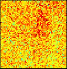
Journal of Biomedical Optics 20(7), 075010 (July 2015)

                Blind deconvolution estimation of fluorescence
                measurements through quadratic programming
                Daniel U. Campos-Delgado,a,* Omar Gutierrez-Navarro,a Edgar R. Arce-Santana,a Melissa C. Skala,b
                Alex J. Walsh,b and Javier A. Joc
                a
                    Universidad Autonoma de San Luis Potosi, Facultad de Ciencias, San Luis Potosi C.P 78290, Mexico
                b
                    Vanderbilt University, Department of Biomedical Engineering, Nashville, Tennessee, United States
                c
                    Texas A&M University, Department of Biomedical Engineering, College Station, Texas, United States

                               Abstract. Time-deconvolution of the instrument response from fluorescence lifetime imaging microscopy (FLIM)
                               data is usually necessary for accurate fluorescence lifetime estimation. In many applications, however, the
                               instrument response is not available. In such cases, a blind deconvolution approach is required. An iterative
                               methodology is proposed to address the blind deconvolution problem departing from a dataset of FLIM mea-
                               surements. A linear combination of a base conformed by Laguerre functions models the fluorescence impulse
                               response of the sample at each spatial point in our formulation. Our blind deconvolution estimation (BDE) algo-
                               rithm is formulated as a quadratic approximation problem, where the decision variables are the samples of the
                               instrument response and the scaling coefficients of the basis functions. In the approximation cost function, there
                               is a bilinear dependence on the decision variables. Hence, due to the nonlinear nature of the estimation process,
                               an alternating least-squares scheme iteratively solves the approximation problem. Our proposal searches for the
                               samples of the instrument response with a global perspective, and the scaling coefficients of the basis functions
                               locally at each spatial point. First, the iterative methodology relies on a least-squares solution for the instrument
                               response, and quadratic programming for the scaling coefficients applied just to a subset of the measured fluo-
                               rescence decays to initially estimate the instrument response to speed up the convergence. After convergence,
                               the final stage computes the fluorescence impulse response at all spatial points. A comprehensive validation
                               stage considers synthetic and experimental FLIM datasets of ex vivo atherosclerotic plaques and human breast
                               cancer cell samples that highlight the advantages of the proposed BDE algorithm under different noise and initial
                               conditions in the iterative scheme and parameters of the proposal. © 2015 Society of Photo-Optical Instrumentation Engineers
                               (SPIE) [DOI: 10.1117/1.JBO.20.7.075010]

                               Keywords: signal processing; fluorescence; deconvolution; digital processing; optimization.
                               Paper 150106R received Feb. 24, 2015; accepted for publication Jun. 29, 2015; published online Jul. 29, 2015.

                1      Introduction                                                                a Laguerre basis.17–19 This process is usually called deconvolu-
                Fluorescence microscopy imaging is a powerful noninvasive                          tion in the FLIM literature.1–4 Once the fluorescence impulse
                technique that allows a biochemical characterization of biologi-                   response has been identified at each spatial point of the sample,
                cal tissue for medical and biophysical applications.1–4 Specifi-                   the lifetime per spectral channel and normalized intensities are
                cally, multispectral fluorescence lifetime imaging microscopy                      used to provide quantitative features for classification purposes
                (m-FLIM) captures the time-resolved response to a laser exci-                      of the m-FLIM dataset.10 Meanwhile, a graphical perspective is
                tation at different spectral channels in order to record the optical               the phasor approach that provides a two-dimensional (2-D) vis-
                emission of synthetic or endogenous fluorophores.5 Different                       ual representation of each spatial point in the dataset by mapping
                studies in the literature have shown the potential of FLIM infor-                  the identified fluorescence impulse response per spectral band.
                mation for providing an early and noninvasive diagnosis tool for                   Classification or linear unmixing can be achieved from this 2-D
                different pathologies, as cardiovascular and dermatology dis-                      representation, as suggested in Ref. 20 and 21.
                eases,6–9 oral precancer conditions,10 colonic dysplasia,11 or                         The main two trends in deconvolution algorithms depend on
                measuring therapeutic responses of anticancer drugs.12,13 In                       the structure of the fluorescence impulse response. The first
                order to provide quantitative evaluations of m-FLIM informa-                       approach assumes a linear combination of exponential functions
                tion, the datasets are first processed to isolate the instrument                   that characterize the response of each fluorophore in the sam-
                signature and extract the intrinsic fluorescence response of                       ple.4,13 Thus, the free parameters in this model are the character-
                the studied sample. Departing from a linear interaction in the                     istic times for the exponential functions and their scaling
                measured fluorescence decay due to the optic excitation, a con-                    coefficients. In this case, the scalings are linear variables in the
                volution model is adopted where the fluorescence impulse                           model, but the characteristic times exhibit a nonlinear depend-
                response denotes the distinctive signature of the sample that is                   ency. Hence, a nonlinear approximation problem is formulated
                usually characterized by a multiexponential model14–16 or by                       to compute the free variables and minimize the prediction error,
                                                                                                   which can be iteratively solved by nonlinear least squares22,23 for

                *Address all correspondence to: Daniel U. Campos-Delgado, E-mail: ducd@
                 fciencias.uaslp.mx                                                                1083-3668/2015/$25.00 © 2015 SPIE

                Journal of Biomedical Optics                                               075010-1                                             July 2015   •   Vol. 20(7)

Downloaded From: https://www.spiedigitallibrary.org/journals/Journal-of-Biomedical-Optics on 18 Jun 2022
Terms of Use: https://www.spiedigitallibrary.org/terms-of-use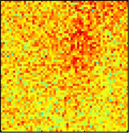
Campos-Delgado et al.: Blind deconvolution estimation of fluorescence measurements through quadratic programming

                each spatial point in the sample. Furthermore, if the character-                   non-negative. Ya∶b ∈ Rðb−aþ1Þ×M represents the block matrix
                istic times are assumed invariant in all the samples, then there                   extracted from Y ∈ RN×M by its rows a to b (1 ≤ a <
                are few parameters involved in the optimization scheme, and                        b ≤ N). For all vectors x ∈ RN and y ∈ RM , T x;y ∈ RN×M
                this concept is called the global approach.14–16 Meanwhile, in                     denotes a toeplitz matrix with x and y⊤ as its first column
                Refs. 24 and 25, by addressing the properties of the optical                       and row, respectively, where the first entry in x and y must
                instrumentation, the exponential profiles can be affected by                       be equal. An N-dimensional vector filled with ones (zeros) is
                uncertainty in the photon counts, which can be modeled as                          represented by 1N (0N ), and IN denotes the identity matrix of
                Poisson noise. Thus, the problem of Poisson–Gaussian param-                        order N. For a random variable x, x ∼ U½a; b represents that
                eter estimation has recently caught the attention of the scientific                x is uniformly distributed in the interval ½a; b (b > a), and x ∼
                community. On the other hand, the second approach for decon-                       N ð0; σ 2 Þ that x is normally distributed with zero mean and vari-
                volution considers that a linear combination of discrete-time
                                                                                                   ance σ 2 .
                Laguerre functions models the fluorescence impulse response;
                this technique is referred to as the model-free scheme. In this
                way, the scaling coefficients of the Laguerre functions are linear                 2       Problem Formulation
                variables in the residual, so a least-squares estimation can be                    First, the deconvolution of FLIM data is expressed in discrete
                followed.17,18 One disadvantage of the Laguerre basis is that                      time by assuming that the measured fluorescence decays and
                for some cases, the resulting fluorescence impulse responses                       instrument response are sampled with a period T over a spatial
                might not have a monotonic decay. Therefore, a constrained                         domain of K points in the dataset.1–3 Therefore, by considering a
                quadratic optimization has to be applied to compute the scaling                    time window of L samples and a causal response,28 the obser-
                coefficients, where the restrictions are imposed to the second-                    vation model for the l’th time sample and k’th spatial point is
                or third-order time derivatives of the resulting fluorescence                      given by
                impulse responses.19
                     One disadvantage of the deconvolution algorithms from the                     yk ½l ¼ u½l⋆hk ½l þ vk ½l                                                (1)
                literature is the requirement of a previous recording of the FLIM
                instrument response. In addition, while computing the deconvo-                                 X
                                                                                                               L−1
                lution methodology, the instrument response has to be carefully                            ¼         u½l − jhk ½j þ vk ½l ∀ l ∈ ½0; L − 1;
                aligned with the fluorescence decay measurements in order to                                   j¼0                                                              (2)
                avoid dead-times, which could be a time-consuming task due
                to noise, and could also bias the lifetime estimations. Hence,                                 k ∈ ½0; K − 1;
                the contribution of this work is to present a blind deconvolution
                estimation (BDE) algorithm that does not require previous                          where yk ½l, u½l, and hk ½l denote the measured fluorescence
                knowledge of the instrument response in the m-FLIM setup.                          decay, instrument response, and fluorescence impulse response
                For this purpose, we consider that the fluorescence impulse                        samples, respectively, ⋆; stands for the convolution operation,
                response is characterized by a linear combination of Laguerre                      and vk ½l represents the random noise related to the instrumen-
                functions. Our BDE algorithm searches for the instrument                           tation or measurement uncertainty. A block diagram of the
                response samples with a global perspective, meanwhile the scal-                    observation model in our formulation is presented in Fig. 1. In
                ing coefficients of the basis functions are computed for each                      our framework, the effect of scattering can be modeled as a
                point in the sample. Since the residual exhibits a bilinear                        scaled factor Ak > 0 of the instrument response in the observa-
                dependency on the decision variables, and alternating least-                       tion model,4,13 i.e., yk ½l ¼ ðhk ½l þ Ak δ½lÞ⋆u½l þ vk ½l, where
                squares (ALS) methodology iteratively estimates the instrument                     δ½l denotes the discrete-time delta function. Therefore, the esti-
                response and scaling variables.26,27 The recurrent steps in the                    mation of the instrument response u½l will not be affected by the
                BDE algorithm rely on constrained quadratic programming                            scattering component, since the structure of the observation
                and least-squares solutions. In this way, our BDE method jointly                   model is not modified with respect to u½l. Although this com-
                provides an estimation of the instrument and fluorescence                          ponent could potentially introduce a distortion of the estimated
                impulse responses in the sample. Our synthetic and experimen-                      impulse response function, that is, ðhk ½l þ Ak δ½lÞ instead of
                tal results with ex vivo atherosclerotic plaques and human breast
                cancer cell samples show that the proposal is robust to uncer-                                                                      y0[l]=h0[l] u[l]+v0[l]
                tainty in the measured fluorescence decays and variations in
                the initial conditions.
                     The notation used in this paper is described next. Scalars are
                                                                                                                                       h0[l]
                denoted by italic letters, and vectors and matrices by lower-case                                                                   y1[l]=h1[l] u[l]+v1[l]
                and upper-case bold letters, respectively. R and Z represent the                       Instrument response

                real and integer numbers, RN N-dimensional real vectors, and
                                                                                                                                       h1[l]
                cardðΩÞ the cardinality of a set Ω. For a real vector x, the trans-
                pose operation                        ⊤
                         pffiffiffiffiffiffiffiffi is denoted by x , the Euclidean norm by                                         u[l]
                              ⊤
                kxk2 ¼ x x, and x ⪰ 0 represents that each component in                                                                             yK-1[l]=hK-1[l] u[l]+vK-1[l]
                the vector is positive or zero. For a square matrix X ∈ RN×N ,
                X i;j represents the element  P in the i’th row and j’th column
                                                                                                                                      hK-1[l]

                (i; j ∈ ½1; N), TrðXÞ ¼ i X i;i denotes the trace operation,
                          pffiffiffiffiffiffiffiffiffiffiffiffiffiffiffiffiffiffi                                                                                       Tissue sample       Measured fluorescence
                kXkF ¼ TrðX⊤ XÞ denotes the Frobenius norm, and kXk∞ ¼
                                                                                                                                                        decay
                       PN
                maxi j¼1 jXi;j j denotes the maximum absolute row sum                              Fig. 1 Fluorescence lifetime imaging microscopy (FLIM) observation
                norm. X ⪰ 0 represents that each component in the matrix is                        model.

                Journal of Biomedical Optics                                               075010-2                                                    July 2015     •   Vol. 20(7)

Downloaded From: https://www.spiedigitallibrary.org/journals/Journal-of-Biomedical-Optics on 18 Jun 2022
Terms of Use: https://www.spiedigitallibrary.org/terms-of-use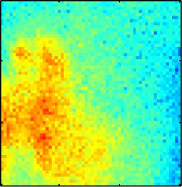
Campos-Delgado et al.: Blind deconvolution estimation of fluorescence measurements through quadratic programming
hk ½l, this a common problem to all deconvolution methods. 2. The fluorescence impulse response hk ½l at each spatial
However, it has been shown that the scattering effect is not sample k and time instant l can be represented by a
significant for endogenous tissue FLIM.29 In general, the decon- linear combination of N discrete-time basis functions
volution formulation is an ill-posed inverse problem that can N−1
fbn ½lgn¼0 also common to all the spatial points.
have multiple solutions.1–3 Therefore, to restrict the search space
and to have a tractable problem, in our formulation, there are Assumption 1 allows to restrict the search among all possible
two key assumptions: instrument responses, and to avoid numerical scaling problems
in the estimation of u½l. Nonetheless, the shape of the resulting
1. The instrument response u½l is common to all K spa- instrument response is not limited as our validation section will
tial points in the dataset, and its samples are non-neg- show. Meanwhile, assumption 2 allows to formulate the estima-
ative and normalized to sum one in time domain, i.e., tion problem as constrained quadratic programming or least-
squares approximations, which can be efficiently solve by
X
L−1
numerical optimization algorithms.23 These two conditions will
u½l ¼ 1 and u½l ≥ 0 ∀ l ∈ ½0; L − 1; be exploited to achieve the blind deconvolution of the dataset as
l¼0
explained next. First, the observation model in Eq. (1) can be
(3) written in a vector notation as
2 3 2 32 3 2 3
yk ½0 u½0 0 ::: 0 hk ½0 vk ½0
6 yk ½1 7 6 u½1 u½0 ::: 0 76 hk ½1 7 6 vk ½1 7
6 7 6 76 7 6 7
6 .. 7¼6 .. .. .. .. 76 .. 7 þ6 .. 7; (4)
4 . 5 4 . . . . 54 . 5 4 . 5
yk ½L − 1 u½L − 1 u½L − 2 : : : u½0 hk ½L − 1 vk ½L − 1
|fflfflfflfflfflfflfflfflffl{zfflfflfflfflfflfflfflfflffl} |fflfflfflfflfflfflfflfflfflfflfflfflfflfflfflfflfflfflfflfflfflfflfflfflfflfflfflfflfflffl{zfflfflfflfflfflfflfflfflfflfflfflfflfflfflfflfflfflfflfflfflfflfflfflfflfflfflfflfflfflffl} |fflfflfflfflfflfflfflfflffl{zfflfflfflfflfflfflfflfflffl} |fflfflfflfflfflfflfflfflffl{zfflfflfflfflfflfflfflfflffl}
yk ∈RL U∈RL×L hk ∈RL vk ∈RL
semidefinite on the third-order derivative (hk0 0 0 ≤ 0).19 The
⇒ yk ¼ Uhk þ vk ∀ k ∈ ½0; K − 1; (5) instantaneous expression in Eq. (7) can be also written in
vector notation to gather all the time samples as
and as a result, the input matrix U has a toeplitz structure30
that does not depend on the spatial location of the sample. hk ¼ Bck ∀ k ∈ ½0; K − 1; (8)
In this matrix formulation, the restrictions in Eq. (3) for
the instrument response can be written as where
2 3
b0 ½0 b1 ½0 ::: bN−1 ½0
kUk∞ ¼ 1 and U⪰0 (6) 6 b0 ½1 b1 ½1 ::: bN−1 ½1 7
6 7
B¼6 .. .. .. .. 7 ∈ RL×N ;
4 . . . . 5
Next, by assumption 2, the fluorescence impulse response
at k’th spatial location is characterized by the scaling coef- b0 ½L − 1 b1 ½L − 1 ::: bN−1 ½L − 1
ficients fck;n gN−1
n¼0 of the basis functions:
(9)
X
N −1
hk ½l ¼ ck;n bn ½l ∀ l ∈ ½0; L − 1; (7) ck ¼ ½ck;0 : : : ck;N−1 ⊤ ∈ RN : (10)
n¼0
In the analysis of FLIM measurements, a well-known basis is
where the coefficients ck;n ∈ R are selected such that the the Laguerre functions:17–19
estimated fluorescence decay matches the measurement,
and the resulting time-response has some smoothness pffiffiffiffiffiffiffiffiffiffiffi X
n
bn ½l ¼ α2ðl−nÞ 1 − α ð−1Þi ðli Þðni Þαn−i ð1 − αÞi
1
property to represent the response of biological sam- i¼0
ples.17–19 The fluorescence impulse responses estimated
∀ n ∈ ½0; N − 1; l ∈ ½0; L − 1; (11)
from FLIM data involve some smoothness properties that
in turn constrain the linear model in Eq. (7).1–3 Hence, the
where α ∈ ð0; 1Þ is a free parameter. Consequently, by consid-
estimated response must be monotonically decreasing to
ering measurement noise, the observation model in Eq. (1) can
have a biological meaning at any spatial point. As a result, be compactly expressed as
the time derivative of the fluorescence impulse response
has to be negative definite (hk0 < 0 ∀ k), but without inflec- yk ¼ UBck þ vk ∀ k ∈ ½0; K − 1: (12)
tion points or curvature changes. Thus, an alternative
restriction is to consider a positive definite condition on By collecting all the spatial measurements in a matrix nota-
the second-order time derivative (hk0 0 > 0), or a negative tion, the following model is obtained
Journal of Biomedical Optics 075010-3 July 2015 • Vol. 20(7)
Downloaded From: https://www.spiedigitallibrary.org/journals/Journal-of-Biomedical-Optics on 18 Jun 2022
Terms of Use: https://www.spiedigitallibrary.org/terms-of-use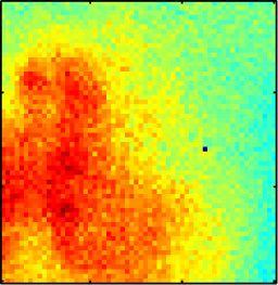
Campos-Delgado et al.: Blind deconvolution estimation of fluorescence measurements through quadratic programming
Y ¼ UBC þ V; (13) yl ¼ ½1 0TL−1 ⊤ ∈ RL : (21)
where To illustrate the toeplitz structure of matrices Uol , the corre-
sponding ones for indices l ¼ 0; 1 and 2 are shown next
Y ¼ ½y0 : : : yK−1 ∈ RL×K ; (14)
Uo0 ¼ IL ;
2 3
N×K
0 0 ::: 0 0
C ¼ ½c0 : : : cN−1 ∈ R ; (15) 6 7
61 0 ::: 0 07
6 7
6 ::: 07
Uo1 ¼ 6 0 1 0 7;
V ¼ ½v0 : : : vK−1 ∈ RL×K : (16) 6. . .. 7
6. . .. .. 7
4. . . . .5
In this way, according to the observation model in Eq. (13), 0 0 ::: 1 0
the blind deconvolution problem is jointly defined as obtaining 2 3
the input and coefficients matrices ðU; CÞ to approximate the 0 0 ::: 0 0 0
6 7
measurements information Y. Hence, our methodology can be 60 0 ::: 0 0 07
formulated as an optimal quadratic approximation problem:23 6 7
61 0 ::: 0 07
6 0 7
Uo2 ¼ 6
60 1
7: (22)
1
6 ::: 0 0 07 7
min kY − UBCk2F ; such that kUk∞ ¼ 1 and U ⪰ 0: 6. .
U;C 2
6 .. .. .. .. .. .. 7
|fflfflfflfflfflfflfflfflfflfflffl{zfflfflfflfflfflfflfflfflfflfflffl}
4 . . . .7 5
J
(17) 0 0 ::: 1 0 0
Therefore, there is a nonlinear interaction in the cost function One advantage of the parametric representation in Eq. (18) is
J between the optimization variables U and C. One important that the normalization condition in Eq. (3) for the instrument
advantage of the previous formulation is that the input matrix U response can be easily incorporated into the optimization formu-
has a toeplitz structure.30 Therefore, to construct this matrix, lation. In this way, the blind deconvolution scheme in Eq. (17)
only L values are needed. Moreover, in FLIM applications, the can be rewritten as
instrument response is a narrow pulse, so there is no need to 2
estimate all the L terms, since many will be zero. Hence, we 1 X
L−1
^
min Y− θl Ul BC
o
consider only the first L^ terms ðL^ < LÞ to represent the instru-
fθl gl¼0 ;C 2
^L−1
l¼0 F
ment response. In this way, the input matrix U in Eq. (4) can be X
parametrized as a linear combination of L^ toeplitz matrices such that θl ¼ 1 and θl ≥ 0 ∀ l ∈ ½0; L^ − 1: (23)
Uol ∈ RL×L l
X
L−1
^
U¼ θl Uol ; (18) 3 Time Restrictions on the Fluorescence
l¼0 Impulse Response
In Ref. 19, to facilitate the computation of the scaling coeffi-
where the parameter θl ¼ u½l represents l’th sample in the cients through numerical optimization, a negative semidefinite
instrument response, and condition (hk0 0 0 ≤ 0) is imposed on the third-order time deriva-
tive (NSC-TOTD). This restriction can be written as a linear
Uol ¼ Txl ;yl ∈ RL×L ; (19) vector inequality for the scaling coefficients ck in Eq. (8) at
k’th spatial location. For this purpose, we employ a numerical
approximation for the TOTD based on the central difference
xl ¼ ½0Tl 1 0TL−l−1 ⊤ ∈ RL ; (20) approach for l’th time instant and k’th spatial point:22
−hk ½l þ 3 þ 8hk ½l þ 2 − 13hk ½l þ 1 þ 13hk ½l − 1 − 8hk ½l − 2 þ hk ½l − 3
hk0 0 0 ½l ¼ ; (24)
8T 3
where to evaluate hk0 0 0 ½l besides the l’th sample, six more 1
A≜ ð−B7∶L þ 8B6∶L−1 − 13B5∶L−2 þ 13B3∶L−4
time samples are needed. Therefore, by using a vector nota- 8T 3
tion, the discrete-time approximation of the TOTD of the − 8B2∶L−5 þ B1∶L−6 Þ ∈ RðL−6Þ×N : (26)
fluorescence impulse response at k’th spatial location is
Following this vector notation, the following linear vector
h 0 0 0 k ¼ Ack ∈ RL−6 ; (25) inequality can represent the time-domain restrictions on the
fluorescence impulse response for the scaling coefficients ck
where at the k’th spatial point:
Journal of Biomedical Optics 075010-4 July 2015 • Vol. 20(7)
Downloaded From: https://www.spiedigitallibrary.org/journals/Journal-of-Biomedical-Optics on 18 Jun 2022
Terms of Use: https://www.spiedigitallibrary.org/terms-of-use
Campos-Delgado et al.: Blind deconvolution estimation of fluorescence measurements through quadratic programming
Ack ≤ 0 ∀ k ∈ ½0; K − 1: (27) where H ¼ B⊤ U⊤ UB, f k ¼ B⊤ U⊤ yk , and A is given by
Eq. (26). Alternatively, the previous optimization problem can
be efficiently solved by its dual formulation23 as a non-negative
4 Quadratic Optimal Approximation least-squares approximation (NNLSA):19
From the previous results in Eqs. (23) and (27), the blind
ξ ¼ arg minkRðA⊤ ξ − f k Þk22 ; (30)
deconvolution problem with time-domain restrictions in the ξ≥0
fluorescence impulse response can be formulated as a quadratic
constrained optimization scheme with linear equality and where R⊤ R ¼ H−1 is obtained by a Cholesky factorization, and
inequality conditions the optimal scaling coefficients are
X
L−1 2 ck ¼ H−1 ð−A⊤ ξ þ f k Þ: (31)
1
^
min Y − θ Uo
BC
l l
fθl gl¼0 ;C 2
^L−1
l¼0 F Since matrices H and A in Eq. (29) are constant for any spatial
X point in the dataset, matrix R can be computed just once for the
such that θl ¼ 1; θl ≥ 0 ∀ l ∈ ½0; L^ − 1;
whole dataset and some terms in Eqs. (30) and (31) can be also
l
precalculated to speed up the numerical implementation. None-
Ack ≤ b ∀ k ∈ ½0; K − 1: (28) theless, the computational time of the estimation process in
Eq. (30) can be raised if the number of spatial locations is large
The proposed optimization scheme in Eq. (28) has a particu- in the FLIM dataset. Nonetheless, this step in the BDE algorithm
lar structure that has not been investigated in the literature so can be further paralleled. In addition, to speed up the convergence
far. For example, in linear unmixing problems or non-negative of the ALS structure, we propose to use a small subset of the
matrix factorization,27,31–33 the measured fluorescence decays whole FLIM dataset in the iterative scheme until convergence is
matrix Y is decomposed as the product of two matrices that reached. At this step, the purpose will be to have a good estimate
have certain properties: positivity and/or normalization condi- of the instrument response. Next, in a final step, provided this
tions. However, in Eq. (28), the parametric structure of the estimated response, the CLSE in Eq. (29) or NNLSA in Eq. (30)
decision variables θl and the presence of the product matrix will be applied to all the spatial points in the FLIM dataset to
Uol B oversee a new formulation. In fact, since the cost function compute the scaling coefficients, and as a result, the fluorescence
in Eq. (28) involves the product of the decision variables impulse responses. We propose an equidistant spatial downsam-
L−1
^
θl l¼0 ; C , and the constraints can be divided into time- pling of size D ∈ Z (D > 1) for the FLIM measurements’ matrix
domain and spatial restrictions, similar to Refs. 26, 27, and 31, Y to obtain its reduced version (column-wise) Y ^ ∈ RL×K^ , with
a solution based on ALS is pursued. Hence, first given an initial K ¼ bK∕Dc, where b c denotes the floor function. As another
^
condition for the unknown parameters alternative, the reduced measurement matrix Y ^ could be computed
by randomly selecting K^ < K columns of the original matrix Y.
h i⊤
θ0 ¼ θ00 ; θ01 ; : : : ; θ0L−1
^ ;
4.2 Instrument Response Estimation
the optimal scaling coefficients ck are calculated for each spatial
location k by an optimal approximation method. The initial In this step, the scaling coefficients’ matrix C is assumed known
instrument response vector θ0 can be chosen from some a priori in the cost function in Eq. (28), and the optimization is com-
information, or as a general square pulse. In this work, we also puted with respect to the parameters fθl gL−1 ^
l¼0 of the instrument
consider a signal that employs the mean spatial measurements of response. In this case, a closed-form solution can be calculated
the FLIM dataset to shape the initial input vector. Next, fixing as will be shown next by using the whole FLIM dataset. First,
the coefficients ck and considering the whole dataset, our pro- the approximation cost function in Eq. P (28) is augmented to
posal calculates the optimal instrument response sequence θ ¼ include the normalization condition l θl ¼ 1 by a Lagrange
½θ0 ; : : : ; θL−1 ⊤ multiplier:23
^ that minimizes the quadratic cost function. This
iterative procedure is repeated until a convergence condition is ⊤
satisfied with respect to the estimation error or when a maximum 1 X
L−1
^
X
L−1
^
J^ ¼ Tr Y− θl Uol BC Y− θi Uoi BC
number of iterations is reached. Next, both optimization steps 2 l¼0 i¼0
are expanded to formulate them as quadratic or least-squares
approximation problems.23 X
L−1
^
þμ θl − 1 (32)
l¼0
4.1 Estimation of Scaling Coefficients
Assuming that the parameters fθl gL−1
^
l¼0 are given, then the input 1 X
L−1 ^
matrix U can be computed from Eq. (4). Since the scaling coef- ¼ TrfY⊤ Yg − θl TrfY⊤ Uol BCg
ficients are estimated for each spatial point k ∈ ½0; K − 1, a 2 l¼0
local constrained least-squares estimation (CLSE) is formulated
X
L−1
^ X
L−1
^
from Eq. (28) as 1 ⊤ ⊤
þ Tr θl C B ðUol Þ⊤ θi Uoi BC
2 l¼0 i¼0
1 1
min kyk − UBck k22 ¼ min c⊤k Hck − f ⊤k ck X
L−1
^
ck 2 ck 2 (29)
þμ θl − 1 (33)
such that Ack ≤ 0; l¼0
Journal of Biomedical Optics 075010-5 July 2015 • Vol. 20(7)
Downloaded From: https://www.spiedigitallibrary.org/journals/Journal-of-Biomedical-Optics on 18 Jun 2022
Terms of Use: https://www.spiedigitallibrary.org/terms-of-use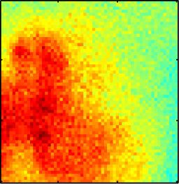
Campos-Delgado et al.: Blind deconvolution estimation of fluorescence measurements through quadratic programming

                where μ ≥ 0 is the Lagrange multiplier related to the equality
                condition. Therefore, the stationary optimality conditions are

                  ∂J^                                                 ∂J^
                      ¼ 0 ∀ m ∈ ½0; L^ − 1                 and           ¼ 0;                  (34)
                 ∂θm                                                  ∂μ

                which result in the following set of equations
                 X
                 L−1
                 ^
                       θl TrfC⊤ B⊤ ðUom Þ⊤ Uol BCg þ μ ¼ TrfY⊤ Uom BCg
                 l¼0
                          |fflfflfflfflfflfflfflfflfflfflfflfflfflfflfflfflfflfflffl{zfflfflfflfflfflfflfflfflfflfflfflfflfflfflfflfflfflfflffl} |fflfflfflfflfflfflfflfflfflffl{zfflfflfflfflfflfflfflfflfflffl}
                                         δm ;l                                  bm
                                                                                                (35)

                    ∀ m ∈ ½0; L^ − 1

                 X
                 L−1
                 ^
                       θl ¼ 1:                                                                  (36)
                 l¼0

                    Consequently, a system with L^ þ 1 linear equations and
                ^L þ 1 unknown variables is obtained
                2                                         32      3 2      3
                   δ0;0        :::       δ1;L−1
                                             ^         1      θ0       b0
                6 .            ..           ..         .. 76 .. 7 6 .. 7
                6 ..                                    .7 6      7 6      7
                6                 .          .            76 . 7 ¼ 6 . 7;                       (37)
                4δ             :::      δL−1;          1  54 θL−1
                                                              ^
                                                                  5 4 bL−1
                                                                       ^
                                                                           5
                   L−1;0
                   ^                     ^   L−1
                                              ^
                     1         :::         1           0      μ        1
                                                                                                              Fig. 2 Block diagram of blind deconvolution estimation.
                                                                    ^
                whose solution provides the optimal parameters θl L−1   l¼0 . If a
                resulting parameter θ^l violates the non-negativity condition,                                IV. Convergence Test: Calculate the estimation error at
                a practical solution inside the iterative process of BDE is to                                    t stage as J t ¼ kY − Ut BCt kF , and evaluate the error
                set it to zero (θ^l ¼ 0) and rescales the parameters to keep the                                  improvement ΔJ t ¼ jJt − J t−1 j with respect to the
                                           P
                normalization condition ( l θl ¼ 1).                                                              previous iteration t − 1. If ΔJ t > κ and t ≤ tmax go to
                                                                                                                  II, otherwise continue.
                                                                                                               V. Estimation of Scaling Coefficients of Laguerre
                4.3      Blind Deconvolution Estimation                                                           Functions on the Whole Dataset: For the complete set
                Finally, by considering the NNLSA in Eq. (30) for the scaling                                     of locations k ∈ ½0; K − 1 with Ut , compute the
                coefficients due to its faster implementation compared to CLSE                                    NNLSA for ctk in Eqs. (30) and (31).
                in Eq. (29), and the closed-form solution for the instrument                                  VI. Compute Final Estimations of Fluorescence Impulse
                response in Eq. (37), the overall BDE algorithm is outlined                                       Responses and Measured Fluorescence Decays: If we
                next (see Fig. 2).
                                                                                                                  assume that the algorithm stops at ^t’th iteration with
                         I. Initialization and Selection of Reduced Dataset:                                      outputs ðθ^t ; C^t Þ, the final estimations are given by
                            Provide the FLIM measurements matrix Y and based
                                                                                                                             θ^tl ; 0 ≤ l ≤ L^ − 1
                            on the selected spatial downsampling D, the reduced                                   u½l
                                                                                                                  ^ ¼                                     ;
                            dataset Y ^ is constructed. Define the number of samples                                         0;    L^ ≤ l ≤ L − 1
                            to be estimated from the instrument response L^ and its                                                            X
                                                                                                                                               N −1
                            initial condition θ0 , a maximum number of iterations                                   h^ k ¼ BC^t ⇒ h^ k ½l ¼          c^tk;n bn ½l
                            tmax , a convergence thresholdfor the                                                                             n¼0
                                                                    estimation error
                            κ, and the basis functions bn ½l N−1   n¼0 to construct
                                                                                                                   ∀ l ∈ ½0; L − 1;      k ∈ ½0; K − 1;
                            B. Set t ¼ 0 and J0 ¼ 106 . From θ0 , compute the                                                                      X
                                                                                                                                                   N −1
                            input matrix U0 from Eq. (4).                                                           y^ k ¼ U^t BC^t ⇒ y^ k ½l ¼          c^tk;n u½l⋆b
                                                                                                                                                                 ^      n ½l;     (38)
                                                                                                                                                   n¼0
                        II. Estimation of Scaling Coefficients of Laguerre
                            Functions: Set t ¼ t þ 1, and for the reduced set of                                  where the input matrix U^t is constructed from θ^t
                            spatial locations k ∈ ½0; K^ − 1 with Ut−1 , compute the                             according to Eq. (4).
                            NNLSA for ctk in Eqs. (30) and (31). Construct the
                            resulting scaling coefficients matrix Ct in Eq. (15).
                       III. Estimation of Instrument Response: Fixing Ct , evalu-                        5    Synthetic and Experimental Validation
                            ate the optimal input parameters θt from Eq. (37). The                       This section presents the validation of the BDE algorithm
                            resulting input matrix Ut is obtained from Eq. (18).                         by considering two cases: synthetic and experimental FLIM

                Journal of Biomedical Optics                                                       075010-6                                                   July 2015    •   Vol. 20(7)

Downloaded From: https://www.spiedigitallibrary.org/journals/Journal-of-Biomedical-Optics on 18 Jun 2022
Terms of Use: https://www.spiedigitallibrary.org/terms-of-use
Campos-Delgado et al.: Blind deconvolution estimation of fluorescence measurements through quadratic programming
PL−1
l¼0 ðu½l − u½lÞ
^ 2
datasets. For both cases, the estimation errors on the instrument
response and measured fluorescence decays will be evaluated, Eu ¼ PL−1
l¼0 ðu½lÞ
2
and in the synthetic experiments, we also quantify the error on PK−1 PL−1
the resulting fluorescence impulse responses. In addition, the ðh ½l − h^ k ½lÞ2
Eh ¼ k¼0
PK−1l¼0 PL−1k
l¼0 ðhk ½lÞ
error on four different initial conditions in the instrument 2
k¼0
response will be analyzed, as well as different scenarios for shot PK−1 PL−1
ðy ½l − y^ k ½lÞ2
noise in the synthetic fluorescence decays.34 Meanwhile, in the Ey ¼ k¼0
PK−1l¼0 PL−1k : (42)
l¼0 ðyk ½lÞ
2
experimental evaluation, we consider a comparison for different k¼0
values of the spatial downsampling factor in step II of BDE, and
a quantification of the lifetime in the fluorescence impulse These three indices ðEu ; Eh ; Ey Þ will give an indication of the
responses. We point out that in the FLIM literature there is no weight of the error energy with respect to the estimated instru-
other algorithm able to perform blind deconvolution that could ment response, fluorescence impulse responses, and measured
provide a comparison benchmark. fluorescence decays in a percentage fashion. Since the construc-
tion of the synthetic datasets involved random samples, we carry
out a Monte Carlo evaluation by implementing the BDE algo-
5.1 Synthetic Evaluation rithm according to the parameters listed in Table 1, whose selec-
tion is explained next. For the Laguerre functions,17,18 the order
The synthetic dataset was generated by considering the mea-
of the approximation was set to 8th for the fluorescence impulse
sured instrument response in Ref. 7 with a sampling interval
responses (N ¼ 8), and their shape parameter was selected as
T ¼ 250 ps and a length of 256 samples (L ¼ 256). This signal
α ¼ 0.85 by a trial and error method. Nonetheless, the two
u½l has a sharp rising time and a subsequent exponential decay
parameters N ¼ 8 and α ¼ 0.85 were pretty robust throughout
(see top plots in Fig. 4), and its normalized to sum 1, i.e.,
P our whole validation stage, since we did not have to modify
l u½l ¼ 1 (assumption 1 in Sec. 2). The fluorescence impulse them for the synthetic and experimental scenarios, although they
response at each spatial point k is modeled as a sum of three
represent different types of FLIM datasets. In the synthetic
exponential functions:
evaluation, 3600 spatial samples were generated by Eqs. (39)
and (40) at different PSNRs (15, 20, 25, and 30 dB), and the
resulting datasets were analyzed by the BDE algorithm,
X
3
−lτ T
hk ½l ¼ ak;i e k;i ∀ k ∈ ½0; K − 1; l ∈ ½0; L − 1; i.e., K ¼ 3600. The spatial downsampling inside the iterative
i¼1
process at step II of the BDE was set to D ¼ 8, i.e., only K^ ¼
K∕D ¼ 450 spatial samples were employed to estimate the
(39)
instrument response. In our evaluation, this reduced number
of measurements K^ was low enough to minimize the complexity
in the estimation of the instrument response, but still provided
where the magnitudes and characteristic times of these functions
enough information to precisely reconstruct it. Meanwhile, the
are randomly chosen for any spatial point, i.e., ak;i ∼ U½0; 50
whole time evolution of the instrument response is captured in
and τk;i ∼ U½0.01; 6 ns ∀ k; i. Next, the synthetic uncorrupted
less than 13.75 ns, so we selected its estimated number of sam-
fluorescence decays yok ½l are computed by applying the convo- ples as L^ ¼ 55, which corresponds to this time by the assigned
lution operator in Eq. (1), i.e., yok ½l ¼ u½l⋆hk ½l. In our evalu- sampling interval T. Finally, to evaluate convergence in the
ation, we included shot noise in the measurements to take into iterative process of the BDE (see Fig. 2), we set the maximum
account uncertainty in the equipment according to the following
model:34
Table 1 Parameters of synthetic dataset and blind deconvolution
qffiffiffiffiffiffiffiffiffi estimation (BDE) implementation during the synthetic evaluation.
yk ½l ¼ yok ½l þ yok ½l · ωk ½l ∀ l ∈ ½0; L − 1; (40)
Parameter Value
where ωk ½l ∼ N ð0; σ 2k Þ represents a normal random variable, Ts 0.250 ns
and its variance σ 2k is selected with respect to a desired peak
K 3600
signal-to-noise ratio (PSNR),
L 256
maxl∈½0;L−1 yok ½l L^ 55
PSNR ¼ 10 log10 ∀ k ∈ ½0; K − 1:
σ 2k D 8
(41)
N 8
α 0.85
By assuming that u½l,
^ h^ k ½l and y^ k ½l denote the estimations
by the BDE algorithm in Eq. (38), we compute three perfor- t max 20
mance metrics to evaluate the accuracy of the methodology κ 0.01
over the whole dataset:
Journal of Biomedical Optics 075010-7 July 2015 • Vol. 20(7)
Downloaded From: https://www.spiedigitallibrary.org/journals/Journal-of-Biomedical-Optics on 18 Jun 2022
Terms of Use: https://www.spiedigitallibrary.org/terms-of-useCampos-Delgado et al.: Blind deconvolution estimation of fluorescence measurements through quadratic programming
PL−1 m 2
number of iterations as tmax ¼ 20 and the convergence preci- and its energy Γ ¼ l¼0 ðy ½lÞ . The initial instrument
sion as κ ¼ 0.01, as a good balance between precision and responses ðu0;1 ; u0;2 ; u0;3 ; u0;4 Þ are analytically described by
complexity in our evaluations. All the data processing was
carried out in MATLAB®. In order to study the performance 1; l ∈ I1
under different initialization signals, four prototypes were u0;1 ½l ¼ ; (44)
0; elsewhere
chosen according to the mean spatial measurement in the
dataset:
8
X
K −1 < 1; l ∈ I1
m 1 u0;2 ½l ¼ 0.1; l ∈ I2 ;
y ½l ¼ yk ½l ∀ l ∈ ½0; L − 1; (43) :
(45)
K k¼0 0; elsewhere
8
< ym;1 ½l; l ∈ ½0; I max
u ½l ¼ ym;2 ½ðl − I max − 1Þ · η; l ∈ ½I max þ 1; I max þ 1 þ ðL − 1 − I max − 1Þ∕η ;
0;3 (46)
:
0; elsewhere
8
< ym;1 ½l; l ∈ ½0; I max • u0;3 stands for an asymmetric pulse generated by the mean
u0;4 ½l ¼ ym;1 ½2I max − l; l ∈ ½I max þ 1; 2I max ; (47) fluorescence decay until its peak value, and its down-
:
0; elsewhere sampled version28 by η factor above the peak; and
• u0;4 depicts a symmetric pulse generated by the mean
where fluorescence decay until its peak value, and its reflection
from this position.
I 1 ¼ fl ∈ ½0; L − 1j0 < ðym ½lÞ2 ∕Γ ≤ Ω1 g; (48)
Therefore, the construction of ðu0;1 ; u0;2 Þ mainly depends on
the time energy distribution of the mean fluorescence decay, and
ðu0;3 ; u0;4 Þ on its increasing and decreasing patterns with respect
I 2 ¼ fl ∈ ½0; L − 1jΩ1 < ðym ½lÞ2 ∕Γ ≤ Ω2 g; (49) to its peak value. In our evaluation, the free parameters were set
to the values Ω1 ¼ 0.35, Ω2 ¼ 0.7, and η ¼ 5 by a trial and error
procedure. These four initial instrument responses ðu0;1 ; u0;2 ;
u0;3 ; u0;4 Þ were later normalized by the condition in Eq. (3).
I max ¼ arg max ym ½l; (50) In addition, our evaluation also considers the deconvolution
l∈½0;L−1 estimation with measured instrument response (DEMIR) u½l
by applying the NNLSA in Eq. (30) (see Fig. 3). Hence,
two new performance indices E0h and E0y can examine the esti-
mation accuracy in the fluorescence impulse response and mea-
ym;1 ½l ¼ ym ½l ∀ l ∈ ½0; I max ; (51) sured fluorescence decays by a direct deconvolution process.
Therefore, E0h and E0y are the two lower bounds in the perfor-
mance of the BDE algorithm for the four initial conditions
ðu0;1 ; u0;2 ; u0;3 ; u0;4 Þ.
ym;2 ½l ¼ ym ½l þ I max þ 1 ∀ l ∈ ½0; L − 1 − I max − 1; Table 2 presents the results of our synthetic evaluation and
(52) shows that the choice of the initial condition has a small effect
Ω1 ; Ω2 ∈ ð0; 1Þ, (Ω1 < Ω2 ), and η ∈ Z (η > 1). In this
way, I 1 and I 2 are the sets of time indices such that
the energy of the mean spatial fluorescence decay meas-
urement ym ½l is below Ω1 %, and between Ω1 % and Ω2 %
of its maximum value, respectively; I max is the time index
for the peak value in the mean measurement; and ym;1 ½l
and ym;2 ½l are the extracted signals below and above the
peak mean measurement, respectively. In this way, the ini-
tial instrument responses take the following shapes:
• u0;1 represents a square pulse with time duration of Ω1 %
the energy of the mean fluorescence decay;
• u0;2 describes a two-step staircase signal with first-step
duration of Ω1 % the energy of the mean fluorescence
decay, and second-step time length between Ω1 % Fig. 3 Block diagram of deconvolution with measured instrument
and Ω2 %; response and deconvolution with approximated instrument response.
Journal of Biomedical Optics 075010-8 July 2015 • Vol. 20(7)
Downloaded From: https://www.spiedigitallibrary.org/journals/Journal-of-Biomedical-Optics on 18 Jun 2022
Terms of Use: https://www.spiedigitallibrary.org/terms-of-useCampos-Delgado et al.: Blind deconvolution estimation of fluorescence measurements through quadratic programming
Table 2 Performance quantification of synthetic datasets for BDE and deconvolution estimation with measured instrument response (DEMIR) with
different initial instrument responses and peak signal-to-noise ratios (PSNRs).
BDE DEMIR
Eu
PSNR (dB) u 0;1 u 0;2 u 0;3 u 0;4 —
15 0.1684 0.1627 0.2559 0.2186
20 0.1470 0.1241 0.2149 0.1782
25 0.1416 0.1286 0.2033 0.1754
30 0.1165 0.1062 0.1636 0.1419
PSNR (dB) Eh E 0h
u 0;1 u 0;2 u 0;3 u 0;4
15 0.0849 0.0848 0.2605 0.2057 0.0663
20 0.0985 0.0856 0.2209 0.1730 0.0515
25 0.1029 0.0954 0.2050 0.1696 0.0482
30 0.0897 0.0836 0.1574 0.1315 0.0443
PSNR (dB) Ey E 0y
u 0;1 u 0;2 u 0;3 u 0;4
15 0.0470 0.0470 0.0470 0.0470 0.0466
20 0.0264 0.0263 0.0264 0.0263 0.0261
25 0.0151 0.0148 0.0202 0.0190 0.0146
30 0.0121 0.0120 0.0153 0.0146 0.0105
on the resulting estimation performance ðEu ; Eh ; Ey Þ for BDE. resulting input estimations by the BDE algorithm for a PSNR
In the experiments, u0;1 and u0;2 consistently achieved the = 15 dB and sample 720, where as expected, all the initial points
best estimations for the instrument and fluorescence impulse qualitatively provided good results. Also, this figure presents
responses ðEu ; Eh Þ at all PSNR values. On the other hand, there a sample of the estimated fluorescence decays and impulse
were no significant performance differences in the estimation in responses for the three initial instrument responses ðu0;1 ; u0;2 ;
the output intensity Ey for all initial responses. Overall, for all u0;3 ; u0;4 Þ. These plots illustrate a good fit to the synthetic data.
initial conditions ðu0;1 ; u0;2 ; u0;3 ; u0;4 Þ, the performance is com-
parable among the metrics in Eq. (42), since the best-case and 5.2 Experimental Evaluation
worst-case errors for the instrument and fluorescence impulse
response estimations ðEu ; Eh Þ were 11%–26%, and 8.5%– 5.2.1 Ex vivo atherosclerotic plaques datasets
26%, respectively. Meanwhile, the estimation error for the fluo-
The first experimental evaluation considers the analysis of mul-
rescence decay Ey varied in a smaller range of 1–5% for all ini-
tispectral FLIM (m-FLIM) datasets of ex vivo atherosclerotic
tial conditions. Consequently, the approximations were more
plaques.7 The temporal resolution of the measurements is
precise with respect to the measured fluorescence decays, which
250 ps. All the measurements include three wavelength bands:
provided smaller estimation errors Ey compared to ðEu ; Eh Þ.
390 20, 452 22.5, and 550 20 nm. Each effective time
The lower bounds ðE0h ; E0y Þ based on DEMIR for the fluores-
trace has a total of L ¼ 167 samples per wavelength. Sixty indi-
cence impulse response and measured fluorescence decay had vidual datasets with 60 × 60 spatial samples were analyzed by
also little variations as 4–7% and 1–5%, respectively. In fact, the BDE algorithm to estimate the instrument and fluorescence
the performance results ðEh ; Ey Þ for BDE with the initial instru- impulse responses and measured fluorescence decays. The same
ment responses u0;1 and u0;2 were comparable to DEMIR in parameters employed in the synthetic evaluation of BDE were
ðE0h ; E0y Þ, which is its lower bound. Another important property considered for the experimental datasets (see Table 1). Since
is that the performance metrics were lightly influenced by the each m-FLIM measurement considers three wavelengths, we
PSNR, where the instrument response and fluorescence impulse only analyze the third wavelength, which has distinct informa-
response estimations ðEu ; Eh Þ were the mostly sensible metrics. tion for classification purposes, i.e., a total of K ¼ 3600 spatial
Nonetheless, the general trend was that as the PSNR increased, points for deconvolution. For all datasets, the instrument
the resulting errors ðEu ; Eh ; Ey Þ had a small decrease for all response has the same time-domain characteristics and it was
initial conditions ðu0;1 ; u0;2 ; u0;3 ; u0;4 Þ. Figure 4 illustrates the recorded for comparison purposes in order to apply DEMIR.
Journal of Biomedical Optics 075010-9 July 2015 • Vol. 20(7)
Downloaded From: https://www.spiedigitallibrary.org/journals/Journal-of-Biomedical-Optics on 18 Jun 2022
Terms of Use: https://www.spiedigitallibrary.org/terms-of-useCampos-Delgado et al.: Blind deconvolution estimation of fluorescence measurements through quadratic programming
Initial input signal u 0,1 Initial input signal u 0,2 Initial input signal u 0,3 Initial input signal u 0,4
Instrument response
Instrument response
Instrument response
Instrument response
0.1 0.1 0.1 0.1 Blind estimation
Measured response
0.05 0.05 0.05 0.05 Initial response
0 0 0 0
0 1 2 0 1 2 0 1 2 0 1 2
Time (sec) −8 Time (sec) −8 Time (sec) −8 Time (sec) −8
x 10 x 10 x 10 x 10
(a) (b) (c) (d)
Sample No. 720 Sample No. 720 Sample No. 720 Sample No. 720
Fluorescence decay
Fluorescence decay
Fluorescence decay
Fluorescence decay
40 40 40 40
Measurement
BDE
20 20 20 20
DEMIR
0 0 0 0
0 5 0 5 0 5 0 5
Time (sec) −8 Time (sec) −8 Time (sec) −8 Time (sec) −8
x 10 x 10 x 10 x 10
(e) (f) (g) (h)
Sample No. 720 Sample No. 720 Sample No. 720 Sample No. 720
Impulse response
Impulse response
Impulse response
Impulse response
60 60 60 60
True response
40 40 40 40 BDE
DEMIR
20 20 20 20
0 0 0 0
0 5 0 5 0 5 0 5
Time (sec) −8 Time (sec) −8 Time (sec) −8 Time (sec) −8
x 10 x 10 x 10 x 10
(i) (j) (k) (l)
Fig. 4 Synthetic evaluation at peak signal-to-noise ratio ðPSNRÞ ¼ 15 dB, where each column corre-
sponds to the initial instrument response ðu 0;1 ; u 0;2 ; u 0;3 ; u 0;4 Þ: (a)-(d) comparison for the instrument
response estimation, (e)-(h) comparison for the fluorescence decay estimation at sample 720, (i)-(l) com-
parison for the fluorescence impulse response estimation at sample 720.
Meanwhile, the instrument response is often approximated as a reconstruction of the instrument response will require a large
pulse created from the rising part of the measured fluorescence PSNR. Nonetheless, these magnitude errors did not affect the
decay by mirroring it around the peak of the fluorescence decay fluorescence impulse response estimations, as the next statistical
pulse, similar to the initial input response u0;4 in Eq. (47). This analysis will show. Next, the shape of the instrument response
approximated instrument response (AIR) pulse is also used for can be quantified by the full width at half maximum (FWHM)
deconvolution in the experimental evaluation. The deconvolu- parameter, and in our experimental setup, the measured value
tion by using the AIR pulse is defined as deconvolution estima- was 1.53 ns. From the results in Fig. 5, the estimations by BDE
tion with approximated instrument response (DEAIR), and it produced a mean FWHM of 1.35 ns for D ¼ 8 and D ¼ 36, but
involves the solution of NNLSA in Eq. (30) for all 60 datasets the AIR pulse produced a large mean value of 2.08 ns. Thus, by
(see Fig. 3). These comparison strategies, DEMIR and DEAIR, comparing to the FWHM of the measured instrument response,
are both based on a Laguerre-base deconvolution, so they the BDE estimation has a percentage error of 11.6%, and the
employ the same expansion order N and shape parameter α AIR pulse of 36.2%. In this way, an advantage is visualized
as in BDE (see Table 1). by BDE estimation compared to the AIR pulse.
In this experimental evaluation, we will study the effect of Figure 6 (top panels) illustrates the boxplots for the metrics
modifying the spatial downsampling that is used to obtain Eu and Ey with the BDE algorithm, and considering DEAIR.
the reduced set of measurements Y. ^ We will consider two As expected, the instrument response estimation by DEAIR
cases, D ¼ 8 and D ¼ 36, i.e., K^ ¼ 3600∕8 ¼ 450 and K^ ¼ presents a larger error compared to BDE. For the 60 datasets,
3600∕36 ¼ 100 spatial samples are used to reconstruct the the mean value of Eu was 11–12% for BDE with both spatial
instrument response at step II of BDE. Figure 5 qualitatively downsamplings, and 49% for DEAIR. Figure 6 (second row)
compares the estimated instrument responses for the 60 datasets illustrates the estimation error for the measured fluorescence
by considering u0;1 as the initial condition, and both spatial decay Ey by using DEMIR. These results show no significant
downsampling factors (D ¼ 8 and D ¼ 36). As a result, a good differences in the DEMIR and BDE output estimation perfor-
estimation is visualized for all datasets and values of D, mances with D ¼ 8 and D ¼ 36, although there is a strong
although some minor discrepancies were observed. These small difference with DEAIR (see second panel in Fig. 6). The mean
magnitude and pulse duration differences in the estimations of value of Ey was 1% for DEMIR and 0.4% for BDE with
Fig. 5 are mainly due to noise in the FLIM dataset, since by the both spatial downsamplings, and 4.5% for DEAIR. Hence,
synthetic results in the previous section (see Table 2), a perfect the BDE method achieved more accurate estimations of the
Journal of Biomedical Optics 075010-10 July 2015 • Vol. 20(7)
Downloaded From: https://www.spiedigitallibrary.org/journals/Journal-of-Biomedical-Optics on 18 Jun 2022
Terms of Use: https://www.spiedigitallibrary.org/terms-of-useCampos-Delgado et al.: Blind deconvolution estimation of fluorescence measurements through quadratic programming
Datasets 1−20 Datasets 1−20
0.2 0.2
Instrument response
Instrument response
Measured response Measured response
0.15 BDE 0.15 BDE
0.1 0.1
0.05 0.05
0 0
0 0.5 1 1.5 2 0 0.5 1 1.5 2
Time (sec) x 10
−8 Time (sec) −8
x 10
(a) (b)
Datasets 21−40 Datasets 21−40
0.2 0.2
Instrument response
Instrument response
Measured response Measured response
0.15 BDE 0.15 BDE
0.1 0.1
0.05 0.05
0 0
0 0.5 1 1.5 2 0 0.5 1 1.5 2
Time (sec) x 10
−8 Time (sec) −8
x 10
(c) (d)
Datasets 41−60 Datasets 41−60
0.2 0.2
Instrument response
Instrument response
Measured response Measured response
0.15 BDE 0.15 BDE
0.1 0.1
0.05 0.05
0 0
0 0.5 1 1.5 2 0 0.5 1 1.5 2
Time (sec) x 10
−8 Time (sec) −8
x 10
(e) (f)
Fig. 5 Experimental evaluation for blind deconvolution estimation (BDE) with datasets of atherosclerotic
plaques: comparison for the instrument response estimation for two spatial downsamplings (left column)
D ¼ 8 and (right column) D ¼ 36, with (a, b) datasets 1–20, (c, d) datasets 21–40, (e, f) datasets 41–60.
Estimation error in instrument response
0.6
0.4
0.2
Eu with DEAIR Eu with BDE (D=8) Eu with BDE (D=36)
Estimation error in measured fluorescence decay
0.06
0.04
0.02
0
Ey with DEMIR Ey with DEAIR Ey with BDE (D=8) Ey with BDE (D=36)
Estimation error in impulse response with DEMIR as ground−truth
0.1
0.05
0
Eh with DEAIR Eh with BDE (D=8) Eh with BDE (D=36)
Estimation error in lifetime with DEMIR as ground−truth
0.15
0.1
0.05
0
El with DEAIR El with BDE (D=8) El with BDE (D=36)
Fig. 6 Experimental evaluation with datasets of atherosclerotic plaques: boxplot results for the metrics
E u and E y by deconvolution estimation with approximated instrument response (DEAIR) and BDE with
spatial downsampling of 8 and 36, E y by deconvolution estimation with measured instrument response
(DEMIR), and E h and E l by DEAIR and BDE taking the results by DEMIR as ground truth.
Journal of Biomedical Optics 075010-11 July 2015 • Vol. 20(7)
Downloaded From: https://www.spiedigitallibrary.org/journals/Journal-of-Biomedical-Optics on 18 Jun 2022
Terms of Use: https://www.spiedigitallibrary.org/terms-of-useCampos-Delgado et al.: Blind deconvolution estimation of fluorescence measurements through quadratic programming
FLIM measurements than with the measured instrument mean lifetime estimation error over the 60 datasets was 6.4% by
response. These statistical results corroborate the qualitative per- DEAIR, and this value was reduced to 3.4% and 4% for BDE
formance of Fig. 5, which illustrates a good estimation for the with D ¼ 8 and D ¼ 36, respectively. Figure 7 presents the
instrument response, since as previously remarked, the pulse resulting lifetime images for datasets 10 and 16 with DEMIR,
shape of the input excitation is correctly estimated. In addition, DEAIR, and BDE (D ¼ 8 and D ¼ 36). The resulting lifetime
the third panel of Fig. 6 shows the estimation error in the fluo- images highlight a good agreement between DEMIR and BDE,
rescence impulse response Eh in Eq. (42) by taking as a ground independently of the spatial downsampling. Consequently, once
truth the DEMIR approximation. Hence, the BDE provides more, the large reduction in the FLIM measurements used to
closer estimations to DEMIR, since the mean error for all data- estimate the instrument response did not produce a significant
sets was 1.3% (D ¼ 8 and D ¼ 36), but for DEAIR the mean loss of accuracy in the BDE algorithm. However, DEAIR shows
error rose to 5.4%. Finally, if h^ lk ∈ RL represents the approxi- some important differences for both datasets, which confirms
mated fluorescence impulse response vector at k’th spatial sam- the advantage of BDE in the deconvolution and lifetime estima-
ple by l strategy ðl ∈ fDEMIR; DEAIR; BDEgÞ, and tk ∈ RL tion processes.
the vector of time samples, the lifetime of the time response λk On the other hand, Table 3 presents the average computa-
can be computed as34 tional time per FLIM dataset in the MATLAB implementation
for the lifetime estimation by using a Pentium Intel Core i7-4770
t⊤k h^ lk 3.5 GHz quad-core processor and 32 GB RAM computer. This
λlk ¼ ∀ k ∈ ½0; K − 1: (53)
1⊤ h^ lk
L
table also shows the average computational time of just the blind
approximation of the instrument response for each dataset, so
Thus, by assuming that the lifetime by DEMIR is the ground the effect of the spatial downsampling can be clearly observed
truth, the percentage error in the estimation by DEAIR and in BDE. Hence, the spatial downsampling provided some reduc-
BDE over the whole dataset is defined as tion in the computational time without compromising the accu-
racy of the estimations, as shown in Fig. 6. Thus, to obtain the
1XK −1 DEMIR
jλk − λDEAIR
k j lifetime image of each dataset, the BDE required in average
EDEAIR
l ¼ ; (54)
K k¼0 λk
DEMIR
11.22 s for a spatial downsample of 36 (D ¼ 36), and just 6.53 s
to estimate the instrument response. Meanwhile, as expected,
the fastest lifetime estimation is achieved by DEMIR since its
1XK −1 DEMIR
jλk − λBDE
k j implementation requires just a direct computation of NNLSA in
EBDE
l ¼ : (55)
K k¼0 λk
DEMIR Eq. (30). The next fastest estimation is DEAIR due to the initial
basic approximation of the instrument response based on the
Thus, the last panel in Fig. 6 presents the results for EDEAIR
l and mean FLIM measurements. Nevertheless, the extra computation
EBDE
l , where once more BDE provided the best estimation. The time by BDE compared to DEAIR is justified to achieve more
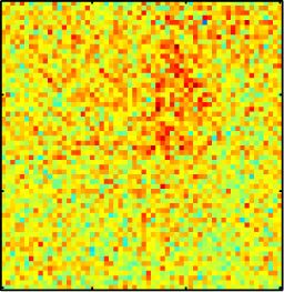
DEMIR DEAIR BDE (D=8) BDE (D=36)
20 20 20 20
Pixel
Pixel
Pixel
Pixel
40 40 40 40
60 60 60 60
20 40 60 20 40 60 20 40 60 20 40 60
Pixel Pixel Pixel Pixel
5 6 5 6 5 6 5 6
−9 −9 −9 −9
x 10 sec x 10 x 10 sec
x 10
sec sec
Dataset 10
DEMIR DEAIR BDE (D=8) BDE (D=36)
20 20 20 20
Pixel
Pixel
Pixel
Pixel
40 40 40 40
60 60 60 60
20 40 60 20 40 60 20 40 60 20 40 60
Pixel Pixel Pixel Pixel
4 6 4 6 4 6 4 6
−9 −9 −9 −9
x 10 x 10 x 10 x 10
sec sec sec sec
Dataset 16
Fig. 7 Experimental evaluation for datasets 10 and 16 of atherosclerotic plaques: lifetimes images that
employ the estimations by DEMIR, DEAIR, and BDE with spatial downsamplings of 8 and 36.
Journal of Biomedical Optics 075010-12 July 2015 • Vol. 20(7)
Downloaded From: https://www.spiedigitallibrary.org/journals/Journal-of-Biomedical-Optics on 18 Jun 2022
Terms of Use: https://www.spiedigitallibrary.org/terms-of-useYou can also read