Back to the Real Economy: The Effects of Risk Mispricing on the Term Premium and Bank Lending
←
→
Page content transcription
If your browser does not render page correctly, please read the page content below
WORKING PAPER SERIES

   Back to the Real Economy: The Effects of Risk
 Mispricing on the Term Premium and Bank Lending

                                                  Kristina Bluwstein
                                                   Bank of England

                                                  Julieta Yung
                                      Federal Deposit Insurance Corporation

                                                    February 2022

                                              FDIC CFR WP 2022-03

                                                      fdic.gov/cfr

The Center for Financial Research (CFR) Working Paper Series allows CFR staff and their coauthors to circulate
preliminary research findings to stimulate discussion and critical comment. Views and opinions expressed in CFR Working
Papers reflect those of the authors and do not necessarily reflect those of the FDIC or the United States. Comments and
suggestions are welcome and should be directed to the authors. References should cite this research as a “FDIC CFR
Working Paper” and should note that findings and conclusions in working papers may be preliminary and subject to
revision.
Back to the Real Economy: The Eects of Risk Mispricing on the
Term Premium and Bank Lending*
Kristina Bluwstein Julieta Yung
This version: January 2022
Abstract
Bond markets can plummet or rally on the back of sentiment-driven reactions which are unrelated
to fundamentals. Therefore, changes in bond prices can not only be interpreted as re
ecting risk but
also mispricing of long-term assets. These perceived risks can often feed back into the economy by
aecting the supply of credit. We construct a DSGE model with heterogeneous banks, asset pricing
rules that generate a time-varying term premium, and introduce bond risk mispricing shocks to study
their eects on the real economy. A risk mispricing shock, in which agents overprice perceived risk,
increases term premia and lowers output by reducing the availability of credit, as banks rebalance
portfolios in favor of longer-term bonds. However, when investors underprice risk, a compressed
term premium leads to a `bad' credit boom that results in a more severe recession once the snapback
occurs.
JEL Codes: E43; E44; E58; G12
Keywords: Stochastic discount factor; risk mispricing; term premium; bank lending
*
We would like to thank Rosalind Bennett, Roberto Billi, Ricardo Caballero, Fabio Canova, Martin Ellison, Mike Joyce,
Christian King, Luisa Lambertini, Chris Martin, Ian Martin, Fred Malherbe, Jordan Pandolfo, Evi Pappa, Ricardo Reis,
Glenn Rudebusch, and Mathias Trabandt, for their insightful comments and feedback, and Chi Hyun Kim and Gabriel
Madeira for their helpful discussions. We also bene
ted from comments made by participants of the 2021 Center for
Financial Research at the FDIC Seminar; 2021 University St. Andrews seminar, 2021 University of Hamburg Quantitative
Economics seminar, 2020 Macro Dynamics Workshop at Colby College; the ASSA 2020 CeMENT Workshop; the Financial
Fragility Session at the 2019 Midwest Macroeconomic Meetings in Michigan State University; the 2019 Women in Macro,
Finance and Economic History Workshop at DIW Berlin; the 2nd Annual NuCamp Conference at Nu
eld College, Oxford;
the XIII Annual Conference on Financial Stability and Banking in Brazil; the 50th Money, Macro, and Finance Conference
in Edinburgh; the 2018 European Economic Association Congress in Cologne; and the Bank of England Seminar series.
The opinions expressed in this article are the sole responsibility of the authors and should not be interpreted as re
ecting
the views of the Federal Deposit Insurance Corporation, the United States, the Bank of England or its Committees.
Bank of England, London EC2R 6DA, UK. Email: kristina.bluwstein@bankofengland.co.uk.
Center for Financial Research, Federal Deposit Insurance Corporation, Washington, DC, 20429, USA. Email:
jyung@fdic.gov.
11 Introduction
Bond markets are generally thought to be driven by fundamentals, with prices re
ecting the expected
future path of short-term assets adjusted for risk. However, markets often plummet or rally on the back
of changes to risk perceptions that do not necessarily stem from underlying actual risks in the economy,
suggesting an occasional mispricing of risks in asset markets (e.g. P
ueger et al., 2020; Lewis et al.,
2021). If market participants overprice or underprice long-term risk, can these `mispricing shocks' aect
credit markets and feed back to the real economy, potentially threatening
nancial stability?
In this paper, we develop a Dynamic Stochastic General Equilibrium (DSGE) model with a rich
nancial sector and bank lending that allows us to investigate the transmission mechanisms through
which bond mispricing leads banks to reassess their lending behavior and ultimately impact economic
activity. To this end, we introduce risk mispricing shocks, which in
uence the compensation for bearing
long-term risk (the term premium) but are unrelated to economic fundamentals. An overpricing of risk
prompts banks to rebalance their portfolios away from private sector loans and towards government
bonds. We
nd that in addition to loans becoming more expensive, a risk mispricing shock also alters
the conditions for bank credit approval, increasing the de-facto required collateral necessary to take out
a loan, making access to credit yet more di
cult. Even without any initial change in underlying eco-
nomic fundamentals, bond mispricing can lead to a pronounced contraction in investment and economic
activity, linking risk mispricing shocks to the real economy via the term premium, through changes in
bank lending decisions.
Our contribution to the literature is three-fold: (1) We combine a banking sector that is subject
to macroprudential regulation with asset pricing rules for long-term bonds in order to investigate how
changes in
nancial markets aect credit allocation to the real economy. (2) The rich structure of our
general equilibrium model and non-linear solution technique enable us to match both macroeconomic
and term premium moments to the data. (3) By introducing a wedge to the stochastic discount factor
of
nancial agents, we model a shock that mimics how
nancial markets and the real economy respond
to the mispricing of long-term risk.
Our framework allows us to investigate lending conditions by dierentiating between a `good' credit
boom driven by economic fundamentals versus a `bad' credit boom driven by agents underpricing risk
in the economy. We
nd that a bad credit boom that leads to a compressed term premium despite
2unchanged fundamentals, is less supportive of economic growth than a good credit boom. Moreover,
once agents correct their mistake and price risk accordingly, the term premium snaps back and output
falls more sharply. A bad credit boom has stronger eects on
nancial markets than a good credit boom.
Nonetheless, while a bad credit boom still drives investment, it is less supportive of consumption with
wages remaining constant, as fundamentals and therefore productivity, remain unchanged. We conclude
by highlighting the implications of dierent macroprudential policies targeted at reducing risk-taking
behavior and promoting
nancial stability.
The paper is structured as follows. Section 2 describes the main assumptions and equations of
the DSGE model that links the real economy and the
nancial sector via the term premium. Section
3 provides more information on the solution method and calibration exercise, the main transmission
mechanism, and the model-implied responses of risk mispricing in the bond markets. It also includes a
detailed robustness section to assess the role of the banking sector and other classic macroeconomic and
nancial shocks in explaining our results. Section 4 explores the richness of our model by simulating
dierent credit boom scenarios to analyze the eectiveness of macroprudential policies in mitigating
nancial instability. Section 5 concludes.
2 A DSGE model with bank lending and risk mispricing
Our main setup is based on Gambacorta and Signoretti (2014)'s model to study augmented monetary
policy rules with bank lending and
rms' balance sheet channels, which combines Iacoviello (2005)'s
type of
nancial frictions with Gerali et al. (2010)'s heterogeneous banking sector. We extend their
framework in several important dimensions in order to structurally analyze the eects of long-term risk
mispricing shocks on the macroeconomy.
First, our model features households that choose consumption, labor, and savings to maximize their
recursive utility with Epstein-Zin preferences as in Rudebusch and Swanson (2012) and Van Binsber-
gen et al. (2012). Intuitively, Epstein-Zin preferences imply that households are not just concerned
with smoothing their consumption once sudden shocks are realized in the short term, but are also con-
cerned with medium- and longer-term changes, allowing long-term risk to play a role in their decision-
making process. As in Gambacorta and Signoretti (2014), competitive entrepreneurs (that are credit
constrained) need to borrow from the banks by providing capital as collateral and therefore produce
3intermediate goods that are sold to retailers. This feature introduces a collateral channel, generating
the Bernanke and Gertler (1995)
nancial-accelerator eect that is subject to an LTV (loan-to-value)
target ratio set by the monetary policy authority. Retailers dierentiate the intermediate goods and
sell them with a mark-up to households, who also own the retailers and keep their pro
ts. In addition,
there are capital producers who buy un-depreciated capital from entrepreneurs and re-sell it for a new
price back to entrepreneurs taking into account a quadratic adjustment cost, necessary to derive the
price for capital. As in Kiyotaki and Moore (1997), capital has many functions in this model and thus
establishes an important feedback mechanism between the economy and the
nancial sector. Capital is
used (i) in the production of intermediate goods, (ii) as a collateral for entrepreneurs' loans, and (iii) as
a source of funds for investment. Therefore capital, along with the LTV ratio and the bank's borrowing
rates, have a crucial impact on consumption and investment decisions made by entrepreneurs, which we
subject to risk mispricing shocks.
Second, following Gambacorta and Signoretti (2014), banks have two branches: a wholesale and
a retail branch, and all debt contracts are indexed in nominal terms in order to focus on the role of
nancial frictions, rather than in
ation. While wholesale banks take deposits from households and
operate under perfect competition, retail banks are monopolistic and give out loans to entrepreneurs
charging a mark-up fee. We modify the banking problem to allow banks to choose between (a) keeping
deposits at the short-term risk-free rate; (b) giving out loans to entrepreneurs and receive pro
ts from
the mark-up they charge over a long-term rate set by asset pricing rules; or (c) investing in long-term
government bonds in the spirit of Gertler and Karadi (2013). Our extension exposes bank loan rates to
risk mispricing shocks that make access to credit more di
cult, a feedback mechanism that we identify
as the loan price channel.
Third, the monetary policy authority determines the capital/asset ratio for banks, sets the LTV
target ratio for entrepreneurs, and follows a more conventional monetary policy rule that minimizes
output and in
ation deviations from their targets, similar to Rudebusch and Swanson (2012). Moreover,
the
scal authority that issues long-term bonds to
nance government spending is modeled exogenously
as a stochastic process.
As in Gertler and Karadi (2011; 2013), Carlstrom et al. (2017), Sims and Wu (2021), and Sims
et al. (2021) we incorporate long-term bonds rather than equity, in a general equilibrium framework
with segmented markets. However, instead of exploring the role of unconventional monetary policies
4on interest rates and ultimately the economy, we focus on mispricing of maturity risk. The fourth and
nal extension of the modeland our key contribution to understanding macro-
nancial linkagesis
therefore the introduction of asset pricing rules where the nominal stochastic discount factor of investors
(which prices long-term assets) is subject to risk mispricing shocks that endogenously elevate or compress
the term premium, above and beyond economic fundamentals. We hence allow investors to misprice
risk by introducing a wedge between the actual price of long-term bonds based on the level of risk in
the economy versus the eective price that is driven by the perception of risk.
2.1 Households
Households maximize their recursive utility function
1
1−ξ 1−ξ
Vt = U (ct , `t ) + βh Et Vt+1 , (1)
where ct is consumption, `t is labor supply, βh is the household's patience discount factor, and ξ is the
Epstein-Zin parameter that captures risk aversion. The intra-period utility function is given by
ct1−ψ `1+φ
U (ct , `t ) = − t , (2)
1−ψ 1+φ
with 1/φ representing the Frisch elasticity of labor and 1/ψ , the intertemporal elasticity of substitution.
Households choose consumption, labor, and deposit their savings (dt ) at wholesale banks, for which they
receive a risk-free gross return 1 + it . They also own retail
rms, which are monopolistic and generate
a pro
t, Jh,t , such that they are subject to the following budget constraint
ct + dt ≤ wt `t + (1 + it−1 )dt−1 + Jh,t , (3)
where wt is the real wage and the short-term nominal interest rate it is set by the monetary policy
authority. The central bank therefore has the potential to directly impact the household decision-
making process, since an increase in the policy rate in Eq. (3) incentivizes households to increase their
savings. The
rst-order condition yields the consumption Euler equation
" ξ #
Vt0
1 βh (1 + it )
= Et , (4)
cψ
t cψ
t+1
Vt+1
5 1
1−ξ 1−ξ
where Vt0 constitutes the certainty equivalent, such that Vt0 = Et Vt+1 . Households also provide
labor to the entrepreneurs for the production of intermediate goods, which follows a standard labor
supply schedule `φt = wt
.
cψ
t
2.2 Entrepreneurs
Entrepreneurs produce goods, employ households, and consume, but also need to borrow from banks
by providing capital as collateral. They form the link between the real economy and the banking sector
and are thus important for generating a feedback loop between the
nancial and macroeconomic sides
of the model. For simplicity, we assume that entrepreneurs have constant relative risk aversion, as
they, unlike households, do not invest or price
nancial assets. The entrepreneurs therefore choose their
consumption (ce,t ), labor demand (`d,t ), and bank loans (be,t ) in order to maximize utility subject to a
budget constraint,
∞
X
max E0 βe log(ce,t ) (5)
{ce,t ,`d,t ,be,t } t=0
ye,t
s.t. ce,t + (1 + ib,t−1 )be,t−1 + wt `d,t + qk,t ke,t ≤ + be,t + qk,t (1 − δk )ke,t−1 ,
xt
where ib,t is the interest rate on bank loans, ke,t is the entrepreneurs' stock of capital that depreciates
1 Pw,t
at rate δk with price qk,t , ye,t is the intermediate output produced by entrepreneurs,
xt = Pt is the
relative competitive price of the intermediate good, and βe represents their patience discount factor.
For small enough shocks, βh >βe makes entrepreneurs more impatient than households, ensuring that
the borrowing constraint is binding and credit is constrained in the economy. The entrepreneurs are
also subject to a borrowing constraint that determines how much they can borrow from banks (i.e. the
collateral channel),
ΩEt [qk,t+1 ke,t (1 − δk )]
be,t ≤ , (6)
1 + ib,t
where Ω is the steady state of the stochastic LTV ratio Ωt , which is an AR(1) process with i.i.d. shock
εΩ,t and variance σΩ . A high LTV ratio implies that banks can lend more for the same amount of
collateral and vice versa.
Entrepreneurs operate under perfect competition and their production function for intermediate
6goods follows a standard Cobb-Douglas form
α
ye,t = At ke,t−1 `1−α
d,t , (7)
where α denotes the capital share and At is the stochastic AR(1) technology process with i.i.d. tech-
nology shock εa,t and variance σa . Their optimal consumption Euler equation,
1 βe (1 + ib,t )
− λe,t = Et , (8)
ce,t ce,t+1
is similar to the households' Euler equation but diers by the Lagrange multiplier on the borrowing
constraint, λe,t , which represents the marginal value of one unit of additional borrowing. Another
important dierence with respect to households is that entrepreneurs face the higher bank loan rate,
ib,t , rather than the short-term risk-free rate, it .
(1−α)ye,t
The labor demand schedule is
`d,t xt = wt and the investment Euler equation equalizes the
marginal bene
t to the marginal cost of saving capital. Since capital serves as collateral, the equa-
tion also depends on the Lagrange multiplier of the borrowing constraint and the LTV ratio,
λe,t Ωt qk,t+1 (1 − δk ) βe qk,t
Et + [qk,t+1 (1 − δk ) + rk,t+1 ] = , (9)
1 + ib,t ce,t+1 ce,t
α−1 1−α
At ke,t−1 `d,t
where rk,t is the return to capital, de
ned as rk,t ≡ α xt .
2.3 Banks
The banking sector is divided into a perfectly competitive wholesale branch and a monopolistic retail
branch. The wholesale sector maximizes bank pro
ts by optimizing the net interest margin between
the wholesale loan rate (iw,t ) and the short-term rate (it ), subject to the quadratic adjustment costs of
deviating from a target capital/asset ratio, ν. The wholesale bank's maximization problem is
2
θ Kb,t
max iw,t Bt − it dt − −ν Kb,t , (10)
{Bt ,dt } 2 Bt
where Bt represents the total assets of the bank and Kb,t is the banks' capital with adjustment cost
θ. As the deposit rate is the same as the risk-free rate, banks' demand for deposits is elastic, with
7the amount of deposits being determined by the households. Wholesale banks are subject to a balance
sheet constraint that can also be interpreted as a capital adequacy/leverage constraint, ensuring all
loans are backed by su
cient bank capital and deposits at the beginning of the period. Combining Eq.
(10) and the banks' balance sheet identity, the
rst-order condition of the wholesale bank collapses to
2
Kb,t Kb,t
iw,t = it − θ Bt −ν Bt .
The retail bank buys the loans from the wholesale bank at price iw,t and uses them either to (i)
lend to the government by purchasing long-term bonds (bl,t ) at rate il,t , or (ii) lend short-term to
entrepreneurs at rate ib,t set by the retail bank. It therefore maximizes pro
ts for Bt = be,t + bl,t ,
max ib,t be,t + il,t bl,t − iw,t Bt , (11)
{ib,t ,bl,t }
with respect to loan demand, be,t = i− b
b,t , where b is the demand elasticity. The
rst order condition of
the retail bank becomes
b
ib,t = il,t , (12)
−1
| b {z }
µb
where µb represents the markup over the long-term rate.
The retail banks have market power, which helps them adjust their lending in response to shocks or
cycles. Notice that, everything else held constant, a shock that increases the long-term rate would also
increase the loan rate charged by retail banks, making access to credit more di
cult for entrepreneurs.
This is eectively the loan price channel through which increases in long-term rates make borrowing
less attractive. Another crucial determinant for the feedback loop between the banking sector and the
real economy is bank capital. Bank capital depreciates at rate δb and accrues from past capital and
retained earnings, Jb,t , Kb,t = Kb,t−1 (1 − δb ) + Jb,t−1 . Since it is pro-cyclical, bank capital worsens
when output declines due to decreasing banks' pro
ts, de
ned as the sum of both the retail bank and
wholesale bank sector pro
ts on loans, long-term bond holdings, and deposits, respectively:
2
θ Kb,t
Jb,t = ib,t be,t + il,t bl,t − it dt − −ν Kb,t . (13)
2 Bt
82.4 Retailers and capital good producers
The monopolistic retailers dierentiate the intermediate goods produced by entrepreneurs at no cost
and sell them with a mark-up. However, retailers face quadratic price adjustment cost, which causes
prices to be sticky (Rotemberg, 1982). The
rst order condition of the retailers generates the classic
New Keynesian Philip's curve
µy,t µy,t 1 ct Yt+1
0=1− + − κπ (πt − 1) πt + βh Et κπ (πt+1 − 1) πt+1 , (14)
µy,t − 1 µy,t − 1 xt ct+1 Yt
1
where the marginal cost is
xt , in
ation is πt = log (Pt /Pt−1 ), κπ represents the degree of price stickiness,
and Yt is total output. The
rm's mark-up, µy,t , is stochastic and follows an AR(1) process with an
autocorrelation coe
cient ρµy and an i.i.d. mark-up shock, εµy,t , with variance σµy .
Capital good producers are perfectly competitive and their main task is to transform the old, un-
depreciated capital from entrepreneurs to new capital without any additional costs. They then resell
the new capital to the entrepreneurs in the next period at price Pk,t , so that the relative price of capital
Pk,t
is qk,t ≡ Pt . In addition, capital producers `invest' in the
nal goods bought from retailers, which are
not consumed by households, and also transform these into new capital.
The
nal goods to capital transformation is subject to quadratic adjustment costs that are parametrized
by κ, the investment (It ) adjustment cost parameter. The
rst-order condition of capital good producers
is
" 2 # " #
It+1 2
κ It It It ce,t It+1
1 = qk,t 1− −1 −κ −1 + βe Et qk,t+1 κ −1 , (15)
2 It−1 It−1 It−1 ce,t+1 It It
with capital, Kt , evolving according to
" 2 #
κ It
Kt = (1 − δk )Kt−1 + 1 − −1 It . (16)
2 It−1
92.5 Monetary policy
Monetary policy follows a standard Taylor rule, in which the central bank sets the one-period nominal
policy rate according to
it = ρi it−1 + (1 − ρi ) i + φπ (πt − π) + φy (yt − y) + εi,t , (17)
where ρi is the interest-rate smoothing coe
cient, i, π, y are the interest rate, in
ation and output
steady states, respectively, and φπ and φy are the in
ation and output monetary policy parameters.
1
εi,t is an i.i.d. monetary policy shock with variance σi .
The monetary policy authority is also responsible for setting a target capital/asset ratio for banks
to avoid an over-leveraging of the economy similar to the Basel Tier 1 leverage ratios. Moreover, the
central bank also sets the LTV target ratio for entrepreneurs.
2.6 Asset pricing equations and risk mispricing
Long-term bonds are default-free securities issued by the
scal authority that pay a geometrically
declining coupon every period in perpetuity.
2 In the traditional
nance literature, the price of a nominal
long-term bond at time t maturing at t + l, pl,t , can be decomposed into the risk-neutral present value
of the bond, pbl,t (i.e. discounted at the risk-free rate), and the covariance between future pay-os and
the bond-pricing stochastic discount factor, m∗t+1 :
pl,t = Et [pl−1,t+1 ] (1 + it )−1 + covt m∗t+1 , pl−1,t+1 .
(18)
| {z } | {z }
risk neutral price=b
pl,t risk discount
1
Fuerst and Mau (2019) pointed out that the exact monetary policy rule speci
cation is important to generate variability
in the term premium in response to macroeconomic shocks. In order to achieve greater variability in the term premium,
the monetary authority should respond to the level of output relative to the steady state rather than the output gap (see
Rudebusch and Swanson, 2012). As an output level rule means the central bank is committing to a contractionary policy
for longer, thus reducing in
ation by more, the term premium is more aected than in the case of an output gap rule.
Hördahl et al. (2008) showed that the degree of interest rate smoothing in the monetary policy rule is also important for
matching bond and macroeconomic moments in their microfounded DSGE framework. Refer to Palomino (2012) for an
analysis of the role of monetary policy regimes and central bank credibility in in
uencing bond risk premia in long-term
bonds.
2
This is equivalent to assuming that long-term bonds are in
nitely-lived consol-style bonds as in Chin et al. (2015). The
purpose of this assumption is to reduce the pricing relationship to just one recursive equation in the model, rather than
having to solve for each maturity level. As shown in Rudebusch and Swanson (2012), this simpli
cation still generates
equivalent results to using ten-year zero-coupon bonds, while signi
cantly reducing the computational burden.
10The
rst term in Eq. (18) corresponds to the asset price in a risk-neutral world with constant con-
covt m∗t+1 , pl−1,t+1 = 0
sumption and linear utility. Notice that if then the price of the long-term
bond is exactly the risk-neutral price.
3 The second term is a risk adjustment, such that a large negative
covariance lowers the price of the bond. Therefore, investors must be compensated to hold assets that
pay poorly during bad times, and vice-versa.
Following the fundamental asset pricing equation, the price of a long-term bond is determined by
the risk-adjusted expected valuation of future pay-os,
pl,t = 1 + δc Et [m∗t+1 pl−1,t+1 ], (19)
where δc is the coupon decay rate that controls the duration of the bond. The continuously compounded
yield for the bond, il,t , and its risk-neutral counterpart, îl,t , are therefore given by
δc pl,t δc p̂l,t
il,t ≡ log and îl,t ≡ log . (20)
pl,t − 1 p̂l,t − 1
As guaranteed by the absence of arbitrage in the bond markets, we compute the nominal term
premium, tpl,t , as the dierence between the yield on the long-term bond and the yield on the equivalent
risk-neutral bond de
ned in Eq. (20):
tpl,t = il,t − îl,t , (21)
hence the term premium re
ects the compensation that risk-averse investors require in order to be
exposed to maturity risk.
A novel feature of our setup is that the valuation of long-term bonds depends on the nominal
stochastic discount factor of the households, subject to risk mispricing, m,t , such that
ψ 0
!ξ
βh ct Vt
m∗t+1 = + m,t , (22)
πt+1 ct+1 Vt+1
where m,t = ρm m,t−1 − εm,t , for εm,t ∼ N (0, σm ) .
The risk mispricing shock enters the stochastic discount factor that prices long-term assets negatively,
3
An important assumption for a positive, time-varying term premium is that the expectations hypothesis therefore
does not hold and households are allowed to be risk averse.
11so that a positive shock lowers the marginal utility growth rate, as prospects for the future valuation
of bonds worsen. Since the demand (and hence price) of long-term bonds goes down, long-term yields
increase via the term premium Eq. (21), as the risk-neutral yield remains unaected by the shock. Notice
that our risk mispricing shock is not a preference shock, as it only enters the nominal stochastic discount
factor that prices bonds, m∗t+1 , i.e. `investors' stochastic discount factor', and not the household's Euler
Eq. (4), acting more like a wedge when it comes to asset prices rather than a fundamental change in
agents' beliefs. This setup is intuitive in that one can imagine how an event or news that trigger a
higher perception of risk might cause investors to change their portfolio allocations immediately but
still not alter their consumption patterns on impact. The idea that there is a wedge between the actual
household stochastic discount factor and the discount factor used to price risk premia has been micro-
founded for example by Barillas and Nimark (2017), who priced bonds subject to speculative behavior
of individual traders, and Ellison and Tischbirek (2021), who decomposed the real term premium at
any maturity into covariances of realized stochastic discount factors and covariances of expectations
of stochastic discount factors which dier due to informational assumptions. Furthermore, we model
risk mispricing as an AR(1) process following the empirical evidence supporting the idea that investors'
perceived changes in the term premium are persistent (see Adrian et al., 2013).
4 This assumption is
also consistent with the literature on uncertainty or credit risk shocks being persistent, as in Christiano
et al. (2014).
2.7 Government sector
For simplicity, we assume that all government spending, Gt , is
nanced exclusively via long-term bonds.
The budget constraint of the
scal authority is thus expressed as current government spending plus the
repayment of interest on the previous debt which cannot exceed the value of current long-term bonds,
bl,t ,
Gt + il,t bl,t−1 = bl,t . (23)
4
Li et al. (2017b) empirically estimated the eect of changes in U.S. term premia, concurrent with changes in implied
U.S. equity volatility and the broad dollar exchange rate index, and found that the eect of a U.S. term premium shock
is persistent with a signi
cant estimate of the autocorrelation coe
cient of 0.78. Using a term structure model of interest
rates, Osterrieder and Schotman (2017) found that when allowing for stronger persistence of interest rate shocks, e.g.
with fractional integration I(0.89), the correlation between risk prices and the spot rate becomes negative, matching the
volatility observed in the data.
12Government spending in Eq. (23) follows a stationary AR(1) process
Gt = (1 − ρg )G + ρg Gt−1 + εg,t , (24)
where G is the steady state value of government consumption, ρg captures the degree of autocorrelation
in
scal policy, and εg,t is a government spending i.i.d. shock with variance σg .5
2.8 Market clearing and aggregation
Goods and labor markets clear with condition γe `d,t = γh `t ; the aggregate banks' balance sheet identity
is Bt = Dt + Kb,t ; and the resource constraint of the economy is
δb Kb,t−1
Yt = Ct + qk,t (Kt − (1 − δk ) Kt−1 ) + + Gt , (25)
πt
as it is a closed economy with Rotemberg adjustment costs, with the following variable de
nitions for
aggregate output (Yt ), consumption (Ct ), capital (Kt ), and deposits (Dt ) in Eq. (25):
Yt = γe ye,t ,
Ct = γh ct + γe ce,t ,
Kt = γe ke,t ,
Dt = γh dt .
3 Results
We describe the solution methods and the baseline calibration for our model in Section 3.1 and compare
the
t of the simulated model moments to the data in Section 3.2. Section 3.3 showcases the impact of
our risk mispricing shock on the economy, focusing on the role of the banking sector in propagating the
shock in Section 3.4. We describe the impact of other classic macroeconomic shocks in Section 3.5 and
evaluate the robustness of our results to dierent parametrization and shock speci
cations in Section
3.6.
5
Note that in this case, government debt is non-explosive, as the transversality (no Ponzi) condition for public debt
applies, i.e., the growth of public debt is smaller than the real interest rate charged on this debt in the in
nite horizon.
133.1 Solution and calibration
Since the dimension of the model is relatively high with 14 state variables, the most feasible option
to solve the model is through perturbation methods.
6 We use third-order solutions and apply pruning
to cut out unstable higher-order explosive terms. The advantage of using third-order solutions is that
the macroeconomic responses remain mostly unchanged, and thus correspond to results in the previous
literature, while the responses for the bond markets can be rendered more realistically. This feature oc-
curs because
rst-order solutions imply that the expectation hypothesis holds and the term premium is
zero, with second-order solutions generating a positive, yet constant term premium, both results incon-
sistent with empirical evidence on risk pricing dynamics (e.g. Shiller, 1979; Campbell, 1987; Longsta,
1990; Cuthbertson, 1996; Piazzesi and Schneider, 2007). The term premium is the compensation that
investors require in order to hold a long-term bond instead of a series of short-term bonds during the
same horizon. A high term premium therefore re
ects a perceived increase in
nancial risk over the
life of a bond. Although unobservable, and therefore di
cult to measure, it has been established in
the literature that this compensation for risk varies throughout time as investors update their beliefs
about the future path of the economy (e.g. Campbell and Shiller, 1991).
7 Only by using third-order
solutions, we manage to capture a time-varying term premium and match empirical bond moments. A
potential disadvantage of this methodology is that the solution method is inherently local and is only
valid around the steady state, so that larger shock variances might lead to more inaccurate results. As
estimation of larger-scale, non-linear models is still di
cult, we follow Rudebusch and Swanson (2012)
and calibrate our model based on standard parameters in the literature and to
t speci
c moments for
both macroeconomic and
nancial variables.
Table 1 reports the values of the calibrated parameters for the baseline model based on previous
estimates for U.S. data, as typically established in the literature. For households and entrepreneurs,
the discount factors are set such that βh implies an annual interest rate of 2% and βh > βe ensures
that entrepreneurs are more impatient as in Gerali et al. (2010) and Gambacorta and Signoretti (2014).
6
Caldara et al. (2012) showed that perturbation methods provide equally accurate solutions to models with recursive
preferences than Chebychev polynomials and value function iterations, but are considerably faster.
7
The term premium is typically estimated or inferred from the term structure of interest rates, forecasts, or surveys of
market participants. Swanson (2007), Rudebusch et al. (2007), and Li et al. (2017a) compared dierent estimates of the
term premium and provide excellent overviews of the challenges faced when measuring the long-term expectation of short
rates. Importantly, despite the disagreement on what the level of the term premium is (e.g. Rudebusch and Swanson,
2012 report a mean of 106 b.p., whereas Adrian et al., 2013 report a mean of 169 b.p. for the 1961/22007/8 period), all
measures broadly agree on the general movements of the term premium and are hence highly correlated.
14For preferences, φ is based on the inverse of the Frisch elasticity being 1/2 and ψ is based on the
intertemporal elasticity of substitution being 0.25, in line with previous micro-founded studies which
have found ψ −1 to be smaller than one (e.g. Vissing-Jørgensen, 2002) so that the utility function is
everywhere positive and the certainty equivalence is well de
ned. We set the Epstein-Zin parameter
|ξ| = 2 to match two term premium moments (mean and standard deviation). Using the constant
relative risk aversion (CRRA) formula in Swanson (2010), this number implies an overall CRRA of
4. This is a remarkable low result in the macro-
nance literature and more consistent with the low
estimates found in the macro literature (see Havranek et al., 2015 for a meta-study).
Table 1: Calibrated parameters
parameters value parameters value parameters value
households
nance shocks
βh 0.995 θ 11 ρa 0.9
βe 0.96 ν 0.09 ρµy 0.9
φ 2 µb 0.0050 ρg 0.9
ψ 4 δc 0.9848 ρΩ 0.9
|ξ| 2 ρi 0.6
ρm 0.9
production monetary policy
µy 1.2 φπ 2 σa 0.007
α 0.3 φy 0.5 σµy 0.005
κπ 28.65 σg 0.005
κ 0.5 steady-state ratios σΩ 0.005
K 10
δk 0.050
Y 3 σi 0.003
G
π 1
Y
0.19 σm 0.005
The production parameters are also standard. The price elasticity of demand is assumed to be 6,
which implies a steady-state markup in the goods market µy = 1.2. The adjustment cost for prices
κπ , modeled via Rotemberg pricing, follows the estimated values by Gambacorta and Signoretti (2014),
as do the adjustment cost for investment κ in Eq. (15), and the adjustment cost for banks θ. The
capital share α is assumed to be 0.3, and δk = 0.05 implies an annual depreciation rate of 20% in Eq.
(16). The banking parameter ν is set to match the Basel capital target ratio of 0.09 and the decay
rate for consol bonds, δc in bond pricing Eq. (19), is set to match the 10-year bond adjusted formula
of Macaulay duration. The monetary policy rule parameters in Eq. (17) re
ect that the central bank
targets both in
ation and output with a stronger weight on in
ation, in line with the literature. The
15shock parameters are also set to standard values, with the persistence of the autoregressive processes
ρ being 0.60.9. The standard deviations of the shocks σ are calibrated between 0.30.7 percentage
points, depending on the volatility of the respective variable when we do the moment matching exercise.
K G
Finally, the steady state capital/output and government spending/output ratios are set to
Y Y
re
ect the long-run macroeconomic relationships between those variables.
3.2 Model
t
To evaluate the
t of the model, we compare both macroeconomic as well as term premium moments
implied by the DSGE model to the data. We use the Hodrick-Prescott
lter to compute the business
cycle component of log quarterly U.S. data for chained GDP, consumption, investment, and labor. We
also include the standard deviations of private and public loan growth for all commercial banks. The
interest rate is the Wu and Xia (2016) annualized shadow Federal Funds rate and in
ation is calculated
using the GDP de
ator. The term premium is the Adrian et al. (2013) nominal ten-year Treasury term
premium from the Federal Reserve Bank of New York. Details and sources can be found in the Data
appendix A.
Table 2 shows the results for the moments observed in the U.S. data during the 19612016 period
in column (a) and the simulated moments using the baseline calibration in column (b). The model
performs very well in matching all the key macroeconomic moments: the standard deviation of output
is under 0.5% of the data variation, and consumption, investment, labor, and in
ation deviate within
20% from their data moments. The variance of the interest rate is slightly further away from its data
standard deviation, as we use the shadow rate and
nd more volatility in the interest rate than is
re
ected empirically, which explains the small discrepancy when matching the variance generated by
the model.
Our calibration also manages to match the term premium within 4% of the data mean and under
0.5% of the data variation.
8 There are two key features that help us match the term premium moments:
Epstein-Zin preferences and third-order solution methods. Firstly, Epstein and Zin (1989) preferences
have the advantage that risk aversion can be modeled independently from the intertemporal elasticity
of substitution. Since Epstein-Zin preferences yield the same results using
rst-order approximations
8
Note that Rudebusch and Swanson (2012) used fourth-order solutions to compute the variances of
nance moments
and achieved a standard deviation of 0.47. One of the reasons we can match bond premium moments without a particularly
large CRRA coe
cient is by having a larger model with more shocks including our new risk mispricing shock.
16as standard utility functions, the model is still able to match macroeconomic moments. However, by
introducing an additional parameter, ξ, the risk aversion of households can now be ampli
ed to also
match the empirical features of bond moments. Fuerst and Mau (2019) explored business cycle moments
for dierent model speci
cations with and without segmented markets and Epstein-Zin preferences, and
found these features to also help deliver a counter-cyclical term premium. We
nd, consistent with their
results and empirical evidence (e.g. Campbell and Cochrane, 1999; Wachter, 2006; Bauer et al., 2012;
Lustig et al., 2014), that the model-implied correlation between output and term premia is 0.61. This
counter-cyclicality suggests that we expect the term premium to rise along with unemployment during
economic downturns and fall during economic upswings, as compensation for risk increases during bad
times and vice versa.
Table 2: Comparing data with simulated model moments
model
(a) (b) (c) (d) (e) (f ) (g) (h)
no risk no bank no TFP no gov. no macro no
nan.
data baseline
mispricing feedback shock shock shocks shock
SD[Yt ] 1.46 1.46 1.18 1.33 0.87 0.88 0.29 1.20
SD[Ct ] 0.85 0.99 0.80 0.81 0.67 0.84 0.25 0.74
SD[It ] 4.08 4.53 2.74 2.86 3.94 2.95 1.87 3.39
SD[`t ] 2.10 1.66 1.53 1.27 1.24 1.32 0.47 1.44
SD[πt ] 2.45 2.36 1.98 2.14 1.31 1.95 0.36 1.93
SD[it ] 3.20 1.76 1.63 0.97 1.50 2.05 0.80 1.56
M [tpl,t ] 1.62 1.69 1.92 1.22 1.41 1.39 1.13 1.50
SD[tpl,t ] 1.19 1.20 0.35 1.09 0.94 0.87 0.70 1.00
Notes: Moments for aggregate output (Yt ), consumption (Ct ), investment (It ), and labor (`t ) are reported in quarterly
percentage points; whereas in
ation (πt ), short-term interest rate (it ), and term premium (tpl,t ) are reported in annual
frequency. The model moments are computed by simulating the data 224 times to be consistent with the duration of
the time series. Refer to the Data appendix A for details on the moments reported in column (a). Column (b) moments
correspond to the model with the baseline calibration from Table 1. Model moments when there is no risk mispricing
shock (εm,t = 0) are reported in column (c), no TFP shock (εa,t = 0) in column (e), no government spending shock
(εg,t = 0) in column (f), no macroeconomic shocks (εa,t = εg,t = εµy,t = 0) in column (g), and no
nancial or LTV ratio
shock (εΩ,t =0) in column (h). Column (d) corresponds to the moments of a model without banking feedback, de
ned
as ib,t = iw,t b−1
b
.
173.3 The impact of a risk mispricing shock: When investors panic
We begin by analyzing how a risk mispricing shock aects the macroeconomy as a temporary, exogenous
change in the nominal stochastic discount factor of investors pricing long-term bonds. Figure 1 reports
the results for a shock that underprices long-term bonds by generating a 90 bps increase in the term
premium (a), a magnitude comparable to the increase experienced from September to October 2008,
during the initial stages of the Global Financial Crisis.
9 This shock lowers the price of long-term bonds
by 8 percent on impact (b) and increases the long-term interest rate by 0.2 percentage points (c), as
participants demand higher compensation due to the perceived elevated risk.
With the long-term rate increasing, purchasing government bonds becomes more pro
table and bank
holdings increase by 0.2 percent (e). Moreover, with the price of bonds decreasing, banks pass on the
elevated rates in form of higher borrowing rates to the private sector, which leads to a decline in loans
to entrepreneurs (d), as borrowers are less willing to take out a loan at a higher rate. This constitutes
a loan price channel, indicating a potential
ight to safety, as risk perceptions in the economy increase.
While the higher return on government debt implies an increase in the demand from banks to purchase
these higher yielding assets (demand eect: price and quantity increase), the increase in the rate for
private loans can be understood as an upwards shift of the bank's supply curve for private loans (supply
eect: price increases and quantity decreases). With higher repayment rates, borrowers are less willing
to borrow and thus reduce the quantity of private loans.
10 Another channel in our model that ampli
es
this eect and reduces borrowing, is the collateral channel. As borrowers are subject to a binding
credit constraint, an increase in the cost of borrowing further reduces the amount that entrepreneurs
can borrow in Eq. (6). We therefore see loans to entrepreneurs decline by more than 0.6 percent over
subsequent quarters, with eects on the private credit market being much more persistent than on the
public sector.
9
We use linear scaling since higher-order solutions allow for dierent shock sizes to result in asymmetric responses.
However, larger variances are also likely to cause oscillating behavior. We indeed
nd a slightly more oscillating response
in bond prices and the short-term interest rate when using a shock variance of 90 bps, indicating that the model solution
might be more unstable for larger variances, although most other responses are both quantitatively and qualitatively very
similar.
10
Notice that modeling commercial and industrial loans as short-term debt aligns closely with the maturity composition
of portfolio allocations by borrowers in the data: More than 90% of commercial loans have a maturity of less than a year
and 70-80% of less than a month (source: E.2 Survey of Terms of Business Lending, Board of Governors of the Federal
Reserve System). In contrast, more than 70% of privately-held public debt has a maturity greater than a year, with
the average maturity of all government debt held by private investors being 5-6 years (source: Table FD-5, US Treasury
Bulletin, Department of the Treasury).
18Figure 1: Impulse responses to risk mispricing shock
Notes: The blue solid line represents the impulse responses to a shock that misprices long-term bonds by rising the
term premium 90 bps, using the baseline calibration from Table 1.
Bond mispricing also has a negative eect on the macroeconomy with output declining by 0.6 percent
on impact (g), returning to the steady state after 4 years. The response in output is mostly driven by
a large fall in investment (i), which drops by more than 2%, rather than consumption (h), which only
falls modestly. We therefore
nd that a risk mispricing shock, unlike a preference shock, does not cause
consumption to respond signi
cantly on impact and only generates a small decline with a trough around
3 years after the shock. These results are consistent with the idea that an increase in the long-term rate
that is orthogonal to the expected path of average future short-term rates, can re
ect mispriced risk in
nancial markets, inducing prices to go down and output and investment to contract. The central bank
reacts to this decline in output by lowering the short-term interest rate on impact (f ), and since prices
19go down, we
nd that the risk mispricing shock behaves similar to a demand shock.
There is recent anecdotal evidence to support the importance of both the loan price and collateral
channels in restricting credit availability during the early 2020 outbreak of the COVID-19 pandemic.
Between March 9th and March 19th, the 10-year U.S. Treasury yield rose by 60 bps, re
ecting a pro-
nounced increase in the Kim and Wright (2005) daily 10-year term premium of almost 40 bps, as
estimated by the Board of Governors.
11 During the following weeks, consumer lending by all commer-
cial banks declined while holdings of Treasuries increased, part of the portfolio-rebalancing strategies
towards safer assets that traditionally follow heightened risk perceptions. At the same time, a higher
percentage of banks tightened their standards for issuing all types of loans (e.g. commercial, consumer,
credit card, mortgage) as well as increased the spread of loan rates over the cost of funds, further re-
stricting the availability of credit between 2020-Q1 and 2020-Q2.
12 While the COVID-19 shock is not
necessarily a bond mispricing shockand was followed by lock-down policies that we do not model in
our frameworkit is a clear recent example of a disruption to the economy whose origins were unrelated
to fundamentals, yet generated sudden portfolio rebalancing changes that at least partially impacted
the availability of credit via the loan price and collateral channels, as described by our model.
Table 2 (c) reports the simulated model moments when we turn o the risk mispricing shock
(εm,t = 0) in Eq. (22). In terms of macroeconomic variables, the model does a worse job at matching
investment
uctuations when this shock is missing, in line with the fact that risk mispricing aects
bank lending and therefore entrepreneurs' ability to get funding and invest. This is more pronounced
than if we were to turn o the other
nancial shock in the model in Table 2 (h), the LTV ratio shock
εΩ,t in Eq. (9), with a more muted decline in the model's ability to match investment volatility. We
also
nd our shock to be important for matching term premia volatility, particularly given our baseline
calibration featuring such a small value for the Epstein-Zin parameter. Otherwise, the ability of our
model to match the remaining moments without risk mispricing shocks is still within 20% of our baseline
speci
cation. In terms of variance decompositions, we compute the empirical moments as we are using
third-order solutions and there is no unique way to decompose the overall variance into the contribution
of individual shocks, because of the interaction eects due to non-linearities. We
nd that the risk
mispricing shock only explains a small fraction of output
uctuations and loans to the government, but
11
See https://www.federalreserve.gov/pubs/feds/2005/200533/200533abs.html.
12
Board of Governors of the Federal Reserve System's April 2020 Senior Loan O
cer Opinion Survey on Bank Lending
Practices release, May 4, 2020, available online at http://www.federalreserve.gov/boarddocs/SnLoanSurvey/.
20is the most important source of
uctuation for loans to entrepreneurs. Although it is only modestly
important for the real economy as a whole (with around 6% of output
uctuations being explained by
it), it represents a quarter of investment movements, and the vast majority of
uctuations in
nancial
markets within the model.
We
nd that, overall, the results of our theoretical model are in line with the previous empirical
literature identifying sizable eects on economic activity resulting from uncertainty shocks (e.g., 1.2%
decline in output in Baker et al., 2016; 1% change in output during expansions and 2% during contrac-
tions in Caggiano et al., 2017; a persistent eect on industrial production Carriero et al., 2018) and in
that our risk mispricing shock seems to correspond with a demand shock (e.g. Leduc and Liu, 2016).
13
Our shock also supports the reduced-form evidence found in the literature that identi
es persistent
eects in macroeconomic variables in response to term premia shocks (e.g. Gil-Alana and Moreno, 2012;
Jardet et al., 2013). Joslin et al. (2014), for example, identi
ed that both economic activity and in
ation
signi
cantly decline when a canonical term structure model of interest rates incorporates macroeconomic
fundamentals beyond the information spanned by the yield curve. Although not a general equilibrium
framework, their model allows future bond prices to be in
uenced by yield curve factors as well as
macroeconomic risks, which in turn account for variation in the term premium.
3.4 The role of banking feedback eects
We further explore the importance of the banking sector in allowing risk mispricing shocks to feed back
to the real economy, by considering a model in which its role is instead more muted. To this end,
we change the banking problem in Eq. (11) such that risk mispricing shocks do not aect the bank's
borrowing rate, eectively removing the feedback mechanism. This implied change in the banking
optimization problem leads to a new retail bank's
rst order condition in which Eq. (12) is now given
by
b
ib,t = iw,t , (26)
−1
| b {z }
µb
13
The term premium is highly correlated with measures of volatility and uncertainty, such as the Merrill Lynch MOVE
Index, which summarizes options-implied expected volatility of Treasury yields and hence represents interest rate risk,
as well as policy and in
ation uncertainty measures as estimated by Baker et al. (2016). We therefore expect the term
premium to be high when investors are more risk averse; output is low; or there is more uncertainty about the future
economic outlook (i.e. the path of interest rates, in
ation,
scal policy).
21such that the long-term rateand therefore risk mispricing shocks impacting term premiano longer
in
uence borrowing rates via the loan price channel. Table 2 (d) displays the simulated model moments
when turning o the banking feedback eect. Although most macro moments remain close to the baseline
results, investment volatility becomes particularly di
cult to match without the feedback mechanism
that arises from the loan price channel, with term premia exhibiting lower mean and volatility than the
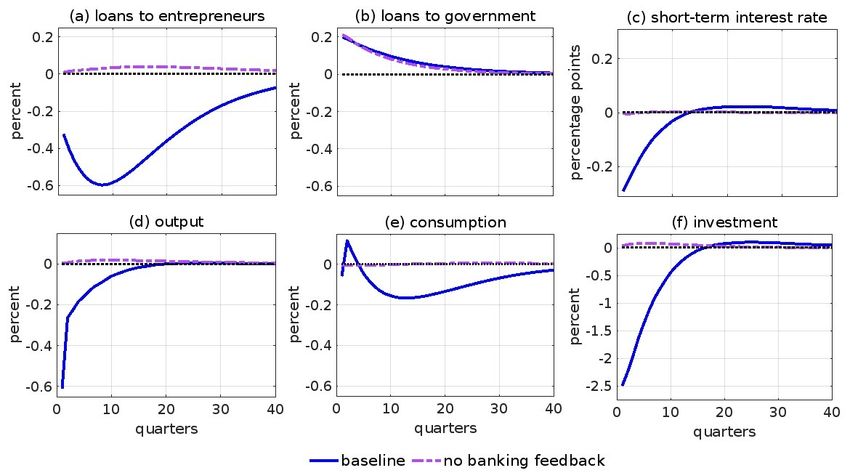
data. Figure 2 highlights the importance of the mechanism through which risk mispricing shocks can
feed back to the real economy. While loans to the government increase at a similar magnitude than
in the baseline model as a result of a risk mispricing shock (b), loans to entrepreneurs are no longer
aected (a), with risk mispricing shocks having no longer any impact on investment (f ) and therefore
output (d), and hence no need for the monetary policy authority to lower the policy rate (c).
Figure 2: Impulse responses to risk mispricing shock with and without banking feedback
Notes: The blue solid line represents the impulse responses to a shock that misprices long-term bonds by rising the
term premium 90 bps, using the baseline calibration from Table 1. The purple dashed line shows the responses to
the same baseline shock after the banking feedback channel is deactivated by not allowing risk mispricing shocks to
enter the banking problem and therefore set the borrowing rates as in Eq. (26).
This mechanism is consistent with anecdotal evidence on bank behavior. The euro area bank lending
survey providing qualitative information on bank loan demand and supply across euro area enterprises
and households, for example, identi
es 'risk perceptions' as one of the most important factors in periods
22of net tightening of credit standards on housing loans and loans to enterprises (Köhler Ulbrich et al.,
2016).
3.5 Other classic macroeconomic shocks
We analyze the impulse responses of traditional macroeconomic shocks, including their eect on the
term premium, to cross-check that their responses are consistent with economic theory and our model
reproduces standard results that are well studied in the literature. The responses to a positive, one stan-
dard deviation technology (a), government spending (b), and monetary policy (c) shocks are reported
in Figure 3.
As is standard in the literature, a technology shockinterpreted as a supply-side shockpersistently
increases output and lowers in
ation, see Figure 3 (a). Consistent with the
ndings outlined in Rude-
busch et al. (2007), a technology shock reveals a negative relationship between output and the term
premium, which declines 15 bps as a result of stronger economic activity associated with higher pro-
ductivity.
14 When we turn o the TFP shock that enters the production function Eq. (7) in Table 2
(e), we
nd TFP shocks to be particularly important for matching output volatility, and to a certain
extent,
uctuations in consumption.
In Figure 3 (b), a one standard deviation, positive government spending shock that represents a
shock on the demand side, raises both output and in
ation on impact as expected, while the term
premium declines by less than a basis point. The small decline in term premium is mechanical, as
the average expected future short-term rate due to the monetary policy response to higher output and
in
ation is higher than the increase in the long-term rate. We therefore
nd almost no impact on the
term premium from such a shock. We can see from Table 2 (f ) that the government spending shock
in Eq. (24) helps account for both
uctuations in output and investment. If we consider our model
without any macroeconomic shocks (i.e., no TFP εa,t , no government spending εg,t , no
rm's mark-up
εµy,t in Eq. (14) shocks), then we are not able to match the volatility of any macroeconomic variable
in the model, see Table 2 (g).
Finally, Figure 3 (c) shows the responses to a one standard deviation contractionary monetary
policy shock. A contractionary monetary policy shock induces less persistent responses and implies, as
14
Huh and Kim (2020) showed that
nancial frictions can play a role in amplifying the eects of TFP shocks on the
term premium and the economy.
23You can also read