Artificial neural network as an effective tool to calculate parameters of positron annihilation lifetime spectra
←
→
Page content transcription
If your browser does not render page correctly, please read the page content below
Artificial neural network as an effective tool to calculate parameters
of positron annihilation lifetime spectra
M. Pietrow∗1 and A. Miaskowski2
1
Institute of Physics, M. Curie-Skłodowska University, Pl. M. Curie-Skłodowskiej 1, 20-031
Lublin, Poland
2
Faculty of Production Engineering, University of Life Sciences, Akademicka 13, 20-950
arXiv:2301.01521v1 [physics.atom-ph] 4 Jan 2023
Lublin, Poland
January 5, 2023
Abstract
The paper presents the application of the multi-layer perceptron regressor model for predicting the
parameters of positron annihilation lifetime spectra using the example of alkanes in the solid phase. A
good agreement of calculation results was found when comparing with the commonly used methods. The
presented method can be used as an alternative quick and accurate tool for decomposition of PALS spectra
in general. The advantages and disadvantages of the new method are discussed.
1 Introduction
Positron Annihilation Lifetime Spectroscopy (PALS) is one of the useful experimental methods using positrons
for studying structural details in a wide spectrum of materials, in particular in the solid state [1]. This method is
based on the annihilation of positrons where their lifetime and annihilation intensity in the sample is dependent
on some properties of the material in the nano scale, including local electron density, bound electron energy,
and the density and size of free volumes in the sample.
Depending on the material, besides the process of direct annihilation, a positron can form a meta-stable atomic
state with an electron, called a positronium (Ps), which can exist in two spin states referred to as para- and
ortho-Ps differing in properties (especially, their lifetimes differ in vacuum by three orders of magnitude) [2]. A
number of conditions must be met for the Ps to be formed in matter. One of them is that free volumes of a
sufficiently large size must be present. For these materials, a Ps is extremely useful in material science since its
lifetime can be related to the size of free volumes [3]. Depending on the structure of the sample, there is possibly
a variety of Ps components which annihilate with characteristic lifetimes. All these populations give their own
account to the positron annihilation spectrum measured experimentally. PALS spectra require decomposition
in the post-measuring procedure of decomposition resulting in both the calculation of lifetimes for particular
species of positrons and the relative amplitudes for these processes (so-called spectrum inversion problem) [4].
Many algorithms used for data processing require assuming an exponential character of positron decay. They
also require fixing the number of components used during the decomposition. For example, the method used by
one of the adequate software, the LT programme [5] or PALSfit [6], consists in fitting the PALS experimental
spectrum to a sum of a given number of exponential functions usually convoluted with the (multi) gaussian
apparatus resolution curve.
The PALS spectra used here were measured for normal alkanes (n-alkanes), i.e. the simplest organic molecules
where carbon atoms form a straight chain of the molecule and are saturated by hydrogen atoms. The n-alkanes
with a different number n of carbon atoms in the molecule form a homologous series described by the general
chemical formula Cn H2n+2 (Cn is used as an abbreviation). Alkanes in the solid phase form molecular crystals
where the trains of elongated molecules are separated by gaps called the inter-lamellar gaps. Ps can be formed
∗ Corresponding Author: marek.pietrow@umcs.pl
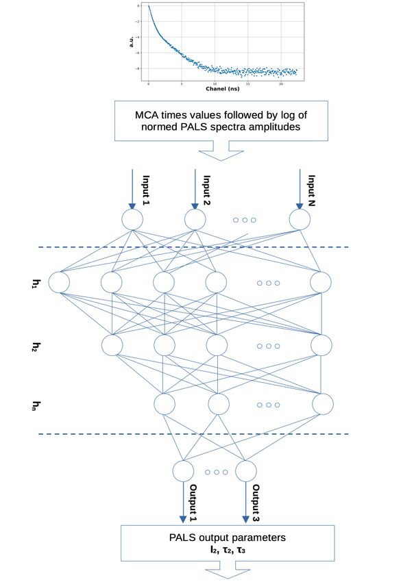
1Figure 1: Schematic view of the MLP applied. The PALS data from consecutive channels of the MCA are
transferred as the amplitudes of the consecutive input neurons Ini . hi denote neurons in the i-th hidden layer
whereas Outi denote output neurons returning chosen PALS decomposition parameters.
in the free volumes made by both the gaps and the spaces generated by changes in the conformation with
temperature [3]. Using the PALS technique, the size of these free volumes can be determined from the lifetime
and the relation between both being given by the Tao-Eldrup formula or its modification [7]. According to our
previous analysis of alkanes carried out with the use of the PALS technique, the best results of the spectrum
decomposition are achieved assuming only one population of ortho- and para-Ps, whereas the ratio of the ortho
to para intensity is fixed at 3/1.
Tools of machine learning like genetic algorithms or artificial neural networks have been used to perform nu-
merical calculations in a variety of aspects in positron science [8, 9, 8, 10, 11, 12]. They have also been used for
unfolding the lifetimes and intensities from PALS spectra [13, 14, 15, 16]. Possibly due to the low computing
power of the hardware and the low time resolution of PALS spectrometers at the time when the neural network
algorithms for decomposition of PALS spectra were proposed, most of the spectra used in these calculations are
simulated by the software but not measured directly. For the same reason, the neural network architecture used
there does not allow changing parameters as much as is allowed by algorithms developed today. Furthermore,
no procedure allowing application for the same calculations of spectra registered for different time constants per
channel has been presented since then. Thus, the preferred software used for spectrum decomposition is still
based on non-linear fitting algorithms which do not include a possibility of establishing the result based on a
multi-spectra set at the same time.
Here, we present an approach to analysis of PALS spectra based on the multi-layer perceptron (MLP) model,
which is one of the tools of machine learning [17]. The model assumes a network of inter-connected neurons
grouped in the input layer (Ini ), the hidden neurons layers (hki ) and the output neurons layer (Outi ), where i
goes over the neurons in a given layer and k numbers the hidden layers. A graphical diagram of the network
used is shown in fig. 1. The numbers of In and Out neurons are determined by the amount of the independent
input data introduced to the network and the data defined to be the results of calculation in a given problem,
respectively. The number of hidden layers and the number of neurons within these layers are set experimentally
to optimise the network to give required results. To each layer (excluding the output layer), one bias neuron is
attached for technical reasons [18]. The tool assumes the learning process first, where the In neurons are fed
with the data for which the result of the Out neurons is known in advance. During this process, the weight
coefficients for pairs of inter-connected neurons are adjusted by an algorithm, so that the output of the MLP
can give results most similar to the expected ones. The MLP becomes to be trained after a number of iterations
of training. Once the MLP results of learning are satisfied, the MLP can be used to calculate the output for
the input data never used in the training process.
2The MLP type of network can be applied to solve the problem of both classification and regression. For the
first group of problems, it is required from the MLP to ascribe the values of the output parameters in the form
of well separated categories. These so-called labels can always be parametrised by a discrete set of numbers.
The problem described in this paper is classified as rather a regression problem (MLPR) where the values of
the output at each Out neuron are characterised by a continuous set of values. Consequently, the output may
contain values approaching these appearing during the learning process but may not necessarily be exactly of
the same value. The internal algorithms of the MLPR allows regarding the learning process as a way of finding
the quasi-continuous output function of input parameters. In our case, based on the data from the PALS spectra
applied as the input values of the perceptron, the MLPR is used for solving the regression problem of finding
the values of key PALS parameters on the output.
2 Method
The scikit-learn library was used to estimate the PALS parameters for alkanes [19]. In our case, the MLP
regressor class (called MLPRegressor ), which belongs to one of the supervised neural network models, was
implemented. In this class, the output is a set of continuous values. It uses the square error as the loss function.
This model optimises the squared error using the Broyden–Fletcher–Goldfarb–Shanno algorithm (LBFGS) [20],
which belongs to quasi-Newton methods. Some MLPRegressor parameters playing a key role are mentioned
below. Their values require to be tuned, especially the alpha hyper-parameter, which helps in avoiding over-
fitting by penalising weights with large magnitudes. A full list of parameters of MLPRegressor is defined in [21].
In the learning process here, we used spectra collected for years from an analog spectrometer for several alkanes
(in the range of C6 – C40 ) measured at several temperatures (-142◦ C – 100◦ C). Irrespective of both the goal of
the particular experiment and the length of the alkane chain used as a sample, the initial assumptions made for
starting the analysis of the spectra made by the LT programme [5] were the same. Each measurement resulting
in the spectra used was performed with a sample prepared in a similar way, i.e. the sample was degassed, and the
rate of cooling or heating was the same. In each case, the measurement at constant temperature took place for
at least one hour which gave some hundreds of thousands of annihilations (the strength of the radioactive source
was similar in each case). During some experiments the temperature was changed stepswise but each spectrum
was collected at constant temperature. The most important issue here is that the post-experimental analysis of
the spectra was conducted under the same general assumptions every time. Especially, for the decomposition of
these spectra, we used LT supposing that the time resolution curve can be approximated by one-gaussian curve.
Every time it was assumed that the annihilation process in the Kapton envelope accounted for 10% (so-called
source correction). Additionally, only one component was always assumed for para- and ortho-Ps, whereas their
intensity ratio was fixed at the value 3/1 (see [22] for details of the experimental procedure).
Taking into account these assumptions, each spectrum was decomposed into three exponential curves for which
the intensities (I) and lifetimes (τ ) were calculated for the following sub-populations of positrons: the free
positron annihilation (I2 , τ2 ), para (I1 , τ1 ), and ortho-Ps (I3 , τ3 )1 . The database collected in this way contained
7973 PALS spectra, wherein about 75% were used in the neural network training process and the rest were used
as a testing set for checking the accuracy of the results given by the learned network.
The number of input neurons is determined by the number of channels of the Multi-channel Analyser (MCA)
module of the PALS spectrometer recording PALS spectra. Furthermore, the number of the output neurons
is related in this model to the number of PALS parameters, which are supposed to be predicted for further
studies of physical processes in the sample. The decomposition of the PALS spectrum made by commonly used
programs, like LT, allows determining (I,τ ) pairs for all assumed components of a given spectrum. However,
often, not all these parameters are needed for further analysis. Furthermore, some of these parameters are
inter-dependent. For example, in the case of PALS spectra for the alkanes discussed here, one assumes that
the spectrum is built up by events from the three populations of positrons mentioned above (τ1 – τ3 , I1 –
I3 parameters). However, from the practical view point, only τ2 , I2 , τ3 , and I3 are then used for studying
physical processes and the structure of the sample. Furthermore, in this case, Ii are inter-dependent and fulfil
the following relations I1 +I2 +I3 =100%2 and I3 /I1 =3. Thus, effectively, the parameters considered as the Out
1 Numbering of the indices is related to the length of τ . The increasing values of the indices correspond to the rising length of
lifetime.
2 Annihilation in Kapton was subtracted in advance.
3Figure 2: Number of spectra (horizontal axis) with a given value of the time constant per channel ∆ (vertical
axis) used as a data set in the presented calculations.
parameters of MLPR are only I2 , τ2 , and τ3 . According to this, we declared in our modelling only three output
neurons for receiving values for these three parameters.
3 Preparation of input and output data
During the PALS measurements, the time constant per channel (∆) varied, depending on the internal properties
and settings of the spectrometer. Most of the data used here were collected with ∆=11.9 ps; however, some
spectra were measured with ∆=11.2 ps, 13.2 ps, 11.6 ps, and 19.5 ps (fig. 2). Therefore, it is important for the
In neurons to code the PALS amplitude samples not in the relation to the channel numbers but in the scale of
time. Hence, in addition to the spectrum amplitudes, the regressor has to learn the times associated with these
amplitudes. Thus, one half of the In neurons is fed with time values for consecutive channels of a spectrum,
whereas the second half is fed with the values of their amplitude. The advantage of the regression approach
applied here is the ability to test spectra measured even for a time sequence that has never appeared in an
extreme case in the training process.
This method requires setting correctly a common zero-time for each spectrum. To achieve this, the original
data from the left slope of the spectrum peak (and only a few points to its right) were used to interpolate the
resolution curve, which is assumed to be in the gaussian form. The position of this peak defines a zero-time
for a spectrum. One-gaussian interpolation is compatible with previous LT analysis assumptions. Based on
the common starting position for all spectra established in this way, the values of time for each channel on the
right to the peak were re-calibrated for each spectrum depending on ∆ for which the spectrum was measured.
Finally, for further analysis, we took the same N number of consecutive channels for each spectrum on the right
to its peak (points pi in fig. 3). The δ parameter shown in fig. 3 denotes the distance (in time units) between
the first point on the right to the peak and the calculated time position of the peak. The number N taken
for further analysis was established experimentally. Finally, the spectrum data for the MLPR input are the N
points pi with their two values: the re-calibrated number of counts in a given channel (see below) and their
re-calibrated times of annihilation.
Then, to minimise errors, the original input data were transformed before application. Each original spectrum
was stored in 8192 channels of MCA. Firstly, starting from the first channel on the right to the spectrum
maximum (p1 in fig. 3), 2k channels were taken from the original spectrum. This means that the spectra
were truncated at about 25 ns of the registration time (varying to some extent, depending on the ∆ for a
given spectrum). Secondly, to smooth random fluctuations, the data were smoothed in most cases. One of the
examples of smoothing is averaging over five consecutive channels. In this case, the number of samples in each
spectrum shrank from the original 2k channels to the amount of 400. Since the In neurons transfer information
about the pair of values – times (t-part) and amplitudes (A-part), 800 input neurons that fed the MLPR with
the data in this case were declared. Thirdly, to standardise the range of the input data values, the set of the
PALS amplitudes was normalised to the maximum value of the amplitude and then logarithmised. According
to these transformations, the A-part data covered the numerical range [-9,0] – fig. 4. Furthermore, to adjust
the range of the values in the t-sector, the values of time were divided by -2.5. As a result, all data transferred
4Figure 3: Schematic view of a peak region of the PALS spectrum. The bullets indicate (t, log(A)) pairs saved
in the MCA channels, whereas the star indicates a position of a peak calculated assuming a gaussian shape
of an apparatus distribution function. Only the points to the right of the star (p1 , p2 , ...) are taken as data
introduced to MLPR. The δ parameter denotes a time distance between the calculated peak and the first point,
whereas ∆ is the time distance between two points.
Figure 4: Input data directed to In neurons can be divided into two sub-sets: t-part which is a set of time
values for points p1 , p2 , ... (see fig. 3) and A-part coding the log function of their normalised amplitudes. In
special cases, these data are smoothed or compressed before use in MLPR.
to the In neurons were in the range of [-10,0].
Additionally, we applied some transformation of the original values for the Out neurons in order to have their
values at each neuron scaled to the same range. Initially, the first output neuron is related to I2 , whereas its
original value range is typically tenths (in % units). The second neuron transfers the information related to
τ2 whose original values are of the order of 0.1 (of ns), whereas the order of τ3 related to the third neuron is
originally 1 (of ns). In order to have the uniform order of numerical values on all Out neurons, the data that
finally feed with them are [I2 /10, τ2 ·10, τ3 ].
The criterion of acceptance of training the network was the best value of the score validation function defined
for this regressor as
(Otrue − Opred )2
P
S =1− N P 2 , (1)
N Otrue
where Otrue , Opred – expected (known) and calculated (predicted) values of the result, respectively [19, 21]. S
is calculated for both the learning and testing sets separately. N here denotes the number of spectra in the
trained or tested set. The optimum value of S is ≈1.
54 Results
The MLPRegressor used in these calculations requires establishing some key parameters [21] influencing the
ability to learn and a speed of the learning process. We performed some tests trying to optimise these param-
eters. The best results we obtained by the settings shown in tab. 1. Both the names and the meaning of the
Table 1: Values of the MLPRegressor parameters applied for producing the final MPLR results.
Parameter value
hidden_layer_sizes = 7×150
activation = relu
solver = lbfgs
alpha = 0.01
learning_rate = invscaling
power_t = 0.5
max_iter = 5e+9
random_state = None
tol = 0.0001
warm_start = True
max_fun = 15000
technical parameters shown in the table are identical to these defined in the routine description [21]. Once
the key parameters of the MLPR were established (especially the solver), we performed tests of credibility
of the network changing the number of hidden layers, the number of neurons within (hidden_layer_sizes
parameter), and the alpha parameter. The results in tab. 2 show examples of the results. For these networks,
we specified the mean validation score parameter for both the training hStr i and testing hSte i sets separately
with their variation δS. Averaging was made over the results of ten runs of the training process for identical
networks differing by initially random weights. We did not notice any rule giving a ratio of the numbers of
neurons that should be declared in the consecutive hidden layers (especially as the number of neurons should
decrease proportionally in the consecutive layers). A few initial examples shown here suggest that the accuracy
of results increases when both the number of hidden layers and the number of neurons inside increase. However,
the last two rows of the table show that a further increase in these parameters does not give better results.
Finally, the network that gave a nearly best result was chosen (marked in bold hStr i in the table). It was checked
for this network that an increase in the iterations of training (max_iter parameter) beyond about 5·109 did
not improve hSi.
Table 2: Valuation score for chosen values of some MLPR parameters. S values are averages over 10 runs with
random initial neuron weights. A nearly optimum case of parameters is placed in a row with S marked in bold.
hidden_layer_sizes max_iter alpha hStr i δStr hSte i δSte
30 × 25 × 15 106 0.7 0.950 0.003 0.942 0.004
3 × 100 108 0.7 0.969 0.005 0.965 0.008
3 × 100 108 0.1 0.974 0.005 0.968 0.008
3 × 100 5· 108 0.1 0.975 0.003 0.976 0.003
4 × 100 108 0.1 0.978 0.004 0.975 0.006
500 × 400 × 300 × 200 5·109 0.01 0.977 0.003 0.974 0.007
7 × 150 5·108 0.01 0.985 0.002 0.975 0.013
500 × 500 × 400 × 400×
5·109 0.01 0.978 0.005 0.977 0.008
×300 × 300 × 200 × 200
9
8 × 500 5·10 0.01 0.982 0.004 0.980 0.005
For several finally tested networks, the spectrum of the magnitude of inter-neurons weights was checked. It
is expected that weights that differ significantly from the average range of values may affect the stability of
the results. In this case, the range of weight values seems to be quite narrow. As shown in fig. 5, the weight
magnitude order (exponent of weights) for the chosen network ranges from 10−5 to 100 , while the relative
number of cases in these subsets changes exponentially. The lack of values outside the narrow set of values
6suggests that self-cleaning of the resultant weights is performed by the MLPRegressor algorithm itself.
Figure 5: Number of cases (log scale) of exponents of weights for a network with 7×100 hidden layers. For this
network, the key parameters are: solver=lbfgs, max_iter=5·1011 , alpha=0.005, learning_rate=invscaling,
and activation=relu.
The number of all PALS spectra used as a database for the network was 7973, and 6500 were used to learn
the output values (training set) by the network, while the rest were used for checking the results of learning
(testing set). Tab. 3 shows a few examples of randomly taken results given by one of the networks finally used.
The results given by the trained network were compared to the expected values known from the LT analysis.
Table 3: Examples of a few randomly taken results of calculations (prediction) of the I2 , τ2 , and τ3 parameters
compared to the expected values calculated by LT. Here, hidden_layer_size=7×150, S=0.985 for both
training and testing sets.
I2 [%] τ2 [ns] τ3 [ns]
Example
expected predicted expected predicted expected predicted
1 68.0 68.8 0.27 0.28 1.21 1.20
2 47.2 47.6 0.38 0.39 3.23 3.18
3 65.4 65.5 0.30 0.29 1.35 1.38
4 78.3 78.3 0.23 0.24 1.11 1.12
5 52.4 52.4 0.35 0.34 2.93 2.93
6 60.5 60.4 0.31 0.30 1.25 1.20
7 59.3 58.8 0.29 0.29 1.19 1.22
8 61.0 62.3 0.30 0.31 1.91 1.91
9 70.2 69.5 0.21 0.21 1.06 1.10
10 39.9 38.8 0.23 0.22 1.15 1.13
Although S for both the trained and tested sets in this case is not the highest one obtained in our tests, the
result of the use of this network is satisfactory in a practical sense because the deviation of the predicted and
expected result is in the range of deviation given by LT itself.
The problem of pre-preparation of spectra for calculations by MLPR is worth mentioning. The main problems
are where the spectrum should be cut and to what extent it is acceptable to smooth the spectra by averaging
their consecutive values. As for the first problem, it was determined by series of runs for which the spectra were
cut at other that mentioned limit of 2k channels that this number of channels was almost the best choice. hSi
was found to worsen in the case of a shorter cut (say, 1.5k channels), and did not improve significantly in the
case of the longer ones (e.g. 3k channels) (but it took longer to compute the result because of an increase in
the number of In neurons).
7The accuracy of the prediction increases when the learning and testing processes are limited to one only ∆ with
all parameters of the network kept constant. In this case, the set of values in the t-part for every spectrum
varies in a much narrower range (only δ changes). In this case, the training process is more effective even if
the size of the training set is reduced. To show this, we separated the set of spectra measured for only one
∆=11.9 ps. Consequently, the whole set of samples under consideration shrank to 4116 members, and 3000 of
them were used for training after the transformations described above. The score S obtained in this case was
much greater than S for an identical network applied to spectra with all possible ∆. The comparison of these
two cases is shown in tab. 4 (the last row of the table). Here, to have the result reliable for networks with
different (random) initial weights, the score was averaged over 30 runs.
Table 4: Comparison of MLPR validation score S for different formats of the input data. Comparison of the
results for ’raw’ data (log of normalised and adjusted data according to the procedure described in section 3)
and data on which the moving average and compressing average (by each 3 and 5 separate spectrum points)
are applied. The result for the network fed with the data collected for one chosen ∆ is added in the last row of
the table.
MLPR and spectra parameters hStr i hSte i
solver=lbfgs unsmoothed data 0.984±0.005 0.963±0.006
Several ∆s
activation=relu moving average 0.984±0.005 0.977±0.007
Ntr =6500 (∼ 80%)
learning_rate=invscaling k=3 0.981±0.005 0.976±0.007
Nte =1473
alpha=0.01, In=800 k=5 0.981±0.006 0.974±0.010
hidden_layer_sizes=7×150 Fixed ∆=11.9 ps
max_iter=5×10⁹ Ntr =3000 (∼73%) k=5 0.993±0.002 0.989±0.003
averaged over 30 trials Nte =1116
The validation score S is sensitive to smoothing the spectrum which reduces to some extent the information
given by the PALS spectrum. In tab. 4, two cases are compared where each 3- and 5-tuples of points of the
spectrum (forming non-overlapping windows) were taken to calculate their average amplitude. For example,
N =3500 points of the initial spectrum are reduced to 700 points when averaging over k=5 points; when the
remainder of the division of N by k is not zero, an integer quotient is taken. hSi calculated for these two cases
shows that both of them give the same results statistically. However, further shrinking the spectrum by setting
k=6 or more produces worse S.
Tab. 4 also shows the S parameter when the moving average is applied during preparation of spectra. The
sampling window applied here is 10. The comparison of this result to the result of calculation with unsmoothed
data shows that the application of the moving average does improve predictions for the testing data set.
5 Conclusions
We have shown in this paper that the easy-to-reach machine learning MLPRegressor tool enhanced with some
programming in Python making some preparation of data, can be used as an alternative method of solving
the problem of inversion of PALS spectra. The main disadvantage of the presented method is the need of
decomposition of training spectra by other software to have Out values for training. Once the training set is
collected and the network is trained, the algorithm works very quickly, giving the result for the tested spectrum.
The training process used here is based on results given by LT, i.e. a method producing results with some
uncertainty itself. The uncertainty produced by the LT is caused by the use of numerical methods to compute
the fit in particular cases. On the other hand, since the MLPR prediction bases on information from a large
set of spectra, this approach seems to be less sensitive to the specific shape of a given spectrum and may
be more accurate in predicting parameters. Furthermore, the presented method seems to be faster than the
referenced ones, since calculations made by a trained network are reduced to simple transformations of matrices
and vectors, which is not demanding computationally and less sensitive to numerical problems.
Although the model presented here is similar to that described in [14] (and repeated in [15]), there are significant
differences indicated in tab. 5. Our experimental data are collected by spectrometers differing in functional
properties, especially differing in time resolution. Even for one spectrometer, this parameter should be re-
calibrated periodically due to changes in experimental conditions, especially temperature. In the algorithm
8Table 5: Comparison of key parameters and results of the MLPR modelling applied in this study (skLearn) and
a three-component spectrum analysis published previously (presented in [14] and [15]).
Pázsit [14] An [15] skLearn
Type of training spectra simulated simulated real (alkanes)
No. of training spectra 575 920 7973
Type of spectra tested simulated simulated, silicon alkanes
No. of test spectra 50 100 (30) 1473
Type of network one-layer perc. one-layer perc. multi-layer perc.
Channel width [ps] 23.2 24.5 some (11.2-19.5)
No. of MCA/taken channels 1500/1500 1024/1024 8192/3500
Approx. no. of counts in spec. 10M 10M ∼400k
Solver backward error prop. backward error prop. some
No. of hidden layers 1 1 some
I2 , τ3 average error [%] 7.3, 1.0 1.07-3.52, 0.55-1.21 -, -
on tested simulated spectra
I2 , τ3 average error [%] -, - -, - 1.03, 1.70
on tested real spectra
presented in [14], the same resolution curve for all spectra is assumed. In our data preparation procedure, the
parameters of the resolution curve are interpolated for each case. Based on this, the δ parameter is calculated
and the value of the shift in time is established for consecutive channels. Although one-gaussian resolution
curve was assumed here, it is possible to extend this algorithm for much more complicated cases where the
distribution curve consisted in a sum of gaussians, for example. As already mentioned in [14], in that case,
a possibility of recognising a distribution function would give compatibility to MELT [23]. Such an extension
requires extending the calculations by applying another neural network, working in advance, which returns the
parameters of the resolution curve in a given case. This problem has been solved by application of a Hopfield
neural network [16]. Taking into account our collection of spectra, it was checked with the use of LT and
(occasionally) with MELT that the apparatus resolution curve is one-gaussian for our spectra. Hence, they do
not allow testing such an extended model.
Furthermore, the MCA module of spectrometers may differ in the time constant per channel ∆. Thus, spectra
used as a training data set may be collected for different channel widths. Taking into account the method
presented in [14] for fixed ∆, the training result is of little use for spectra collected with another ∆. Oppositely,
we have shown the possibility of application of an improved algorithm to data collected for different ∆s. The
data collected from many spectrometers may contribute to a large training data set, which allows solving the
inversion problem for any PALS spectrum and, thus, may be a universal tool that can be used in different
laboratories. Although the set of ∆ used here is small, the accuracy of the results is quite good. To use this
tool to determine the real-world spectrum parameters, the training process should be extended by adding the
spectra measured for a wider range of ∆.
For greater generalisation, it is possible in principle to attach spectra collected for other compounds to the
training data set. For consistency, it suffices for a training database to keep the same number of components
(three here) in spectrum decomposition. However, in practice, some incompatibilities of the spectra for different
compounds may arise because decomposition into a few exponential processes is probably always a simplification
of a real case where some distribution of the size and shape of free volumes should be taken into account as well
as other Ps formation details.
Although the approach presented here is reduced to the analysis of alkanes solely, the algorithm can be applied
in calculation of PALS parameters of other types of samples as well.
References
[1] D. Manara, A. Seibert, et al. Positron annihilation spectroscopy. In M.H.A. Piro, editor, Advances in
Nuclear Fuel Chemistry, chapter 2.3.5, pages 126–131. Elsevier Ltd., Woodhead Publishing, 2020.
[2] W. Greiner and J. Reinhardt. Field Quantization. Springer, 2013.
9[3] T. Goworek. Positronium as a probe of small free volumes in crystals, polymers and porous media. Ann.
Univ. Mariae Curie Sklodowska, sectio AA – Chemia, LXIX:1–110, 2014.
[4] Y.C. Jean, J.D. Van Horn, W-S Hung, and K-R Lee. Perspective of positron annihilation spectroscopy in
polymers. Macromolecules, 46:7133–7145, 2013.
[5] J. Kansy. Microcomputer program for analysis of positron annihilation lifetime spectra. Nucl. Instr. Meth.
A, 374:235–244, 1996.
[6] Jens V. Olsen, Peter Kirkegaard, Niels Jørgen Pedersen, and Morten Mostgaard Eldrup. Palsfit: A new
program for the evaluation of positron lifetime spectra. Physica Status Solidi (C) Current Topics in Solid
State Physics, 4(10):4004–4006, 2007.
[7] K. Wada and T. Hyodo. A simple shape-free model for pore-size estimation with positron annihilation
lifetime spectroscopy. J. Phys. Conf. Ser., 443:012003, 2013.
[8] J. Jegal, D. Jeong, E.S. Seo, et al. Convolutional neural network-based reconstruction for positronium
annihilation localization. Sci Rep, 12:8531, 2022.
[9] J.L. Herraiz, A. Bembibre, and A. López-Montes. Deep-learning based positron range correction of pet
images. Applied Sciences, 11(1), 2021.
[10] M. Wędrowski. Artificial neural network based position estimation in positron emission tomography. PhD
thesis, Interuniversity Institute for High Energies, Vrije Universiteit Brussel, Belgium, 2010.
[11] W.J. Whiteley. Deep Learning in Positron Emission Tomography ImageDeep Learning in Positron Emission
Tomography Image ReconstructionReconstruction. PhD thesis, University of Tennessee, Knoxville, U.S.A.,
2020.
[12] D. Petschke and T.E.M. Staab. A supervised machine learning approach using naive gaussian bayes clas-
sification for shape-sensitive detector pulse discrimination in positron annihilation lifetime spectroscopy
(pals). Nucl. Instrum. Methods. Phys. Res. B, 947:162742, 2019.
[13] N.H.T. Lemes, J.P. Braga, and J.C. Belchior. Applications of genetic algorithms for inverting positron
lifetime spectrum. Chem. Phys. Lett., 412(4):353–358, 2005.
[14] I. Pázsit, R. Chakarova, P Lindén, and F. Maurer. Unfolding positron lifetime spectra with neural networks.
Appl. Surf. Sci., 149:97–102, 08 1999.
[15] R. An, J. Zhang, W. Kong, and B-J. Ye. The application of artificial neural networks to the inversion of
the positron lifetime spectrum. Chinese Physics B, 21(11):117803, nov 2012.
[16] V.C. Viterbo, J.P. Braga, A.P. Braga, and M.B. de Almeida. Inversion of simulated positron annihilation
lifetime spectrum using a neural network. J. Chem. Inf. Comput. Sci., 41:309–313, 2001.
[17] G. Rebala, A. Ravi, and S. Churiwala. An Introduction to Machine Learning. Springer Nature, 2019.
[18] J. Heaton. Introduction to the Math of Neuroal Networks. Heaton Res., 2012.
[19] F. Pedregosa, G. Varoquaux, A. Gramfort, V. Michel, B. Thirion, O. Grisel, M. Blondel, P. Prettenhofer,
R. Weiss, V. Dubourg, et al. Scikit-learn: Machine learning in python. J. Mach. Learn. Res., 12:2825–2830,
2011.
[20] Broyden–fletcher–goldfarb–shanno algorithm. https://en.wikipedia.org/wiki/
Broyden-Fletcher-Goldfarb-Shanno_algorithm. Accessed: 2022-11-20.
[21] sklearn.neural_network.mlpregressor. https://scikit-learn.org/stable/modules/generated/
sklearn.neural_network.MLPRegressor.html.
[22] T. Goworek, M. Pietrow, R. Zaleski, and B. Zgardzińska. Positronium in high temperature phases of
long-chain even n-alkanes. Chem. Phys., 355:123–129, 2009.
[23] A. Shukla, M. Peter, and L. Hoffmann. Analysis of positron lifetime spectra using quantified maximum
entropy and a general linear filter. Nuclear Instruments and Methods in Physics Research Section A:
Accelerators, Spectrometers, Detectors and Associated Equipment, 335(1):310–317, 1993.
10You can also read


