Wind plants can impact long term local atmospheric conditions
←
→
Page content transcription
If your browser does not render page correctly, please read the page content below

www.nature.com/scientificreports
OPEN Wind plants can impact long‑term
local atmospheric conditions
Nicola Bodini1*, Julie K. Lundquist1,2,3 & Patrick Moriarty1
Long-term weather and climate observatories can be affected by the changing environments in their
vicinity, such as the growth of urban areas or changing vegetation. Wind plants can also impact local
atmospheric conditions through their wakes, characterized by reduced wind speed and increased
turbulence. We explore the extent to which the wind plants near an atmospheric measurement site in
the central United States have affected their long-term measurements. Both direct observations and
mesoscale numerical weather prediction simulations demonstrate how the wind plants induce a wind
deficit aloft, especially in stable conditions, and a wind speed acceleration near the surface, which
extend ∼ 30 km downwind of the wind plant. Turbulence kinetic energy is significantly enhanced
within the wind plant wake in stable conditions, with near-surface observations seeing an increase of
more than 30% a few kilometers downwind of the plants.
As wind flows past the rotating blades of a wind turbine, some of its momentum is devoted to moving the
blades and generating electricity. As a result, the downwind flow is slower and more t urbulent1,2. Assessing the
characteristics of this wake has been identified as one of the grand challenges that wind energy science needs to
face to drive innovation in the sector and meet future energy demand3. Wakes are particularly complex: their
characteristics depend on the incoming wind speed, wind direction, and turbulence, as well as turbine operation
and associated parameters. In convective conditions, wakes tend to be eroded rapidly by ambient turbulence4–6.
In stably stratified conditions with weak turbulence, wakes tend to exhibit a large wind speed deficit and persist
for long distances d ownwind7,8. For example, aggregated wakes from multiple turbines, i.e., wind plant wakes,
can extend more than 50 km downwind of a wind plant, offshore in stable c onditions9. In addition to the wind
speed deficit and the enhancement of turbulence at the heights above the surface corresponding to the wind
turbine rotor, wakes can affect local surface conditions. For example, nocturnal surface temperatures can rise
because of turbine-induced mixing of the nocturnal i nversion10–12.
Long-term meteorological measurements in the vicinity of wind plants can also be affected by wind
plant wakes. Just as the “urban heat island” effect affects meteorological measurements in and near cities and
towns13,14, the “wind plant wake” effect can affect measurements of winds, turbulence, and temperature near
wind plants9,11,15. But the effects of the wakes on local meteorological measurements are generally difficult to
discern because the magnitude and orientation of the wind plant wake change with wind speed, wind direction,
and atmospheric stability as well as the height of the boundary layer8,16; therefore, an accurate assessment of the
effects of wind plants on local atmospheric conditions, both aloft and at the surface, is of primary importance for
wind plant d esign17, operational m
anagement18 and for assessing applicability of and uncertainty in the use of
meteorological observations near a wind plant. In addition, the importance of such an accurate characterization
will continue to increase because wind energy deployment is expected to keep increasing worldwide. In fact,
the global installed wind capacity experienced an unprecedented increase by 91% from 2012 to 2017. Future
estimates predict an additional growth by a factor of 5 by 203519 and a factor of 10 by 205020, which will lead the
wind energy industry reaching the trillion-dollar scale.
The US Department of Energy’s Atmospheric Radiation Measurement (ARM) program’s Southern Great
Plains (SGP) site, near Lamont, Oklahoma, is an optimal candidate location for such an assessment. In fact, the
site offers a unique array of long-term atmospheric instrumentation. Further, it has been gradually surrounded
by wind plants over the last 15 years. Several studies have analyzed the wind flow at the SGP, for example, by
looking at the frequent low-level jets21,22 or by proposing improved wind speed extrapolation t echniques23,24.
The Lower Atmospheric Boundary Layer Experiment (LABLE) short-term intensive field c ampaign25 has led
to better characterization of the boundary layer processes at the site26,27. Baidya Roy et al.10 simulated the effect
of a hypothetical wind plant in the region using short-term coarse-resolution Regional Atmospheric Modeling
System (RAMS) mesoscale s imulations28. However, recent s tudies29 stressed the importance of using mesoscale
1
National Renewable Energy Laboratory, Golden 80401, CO, USA. 2Department of Atmospheric and Oceanic
Sciences, University of Colorado Boulder, Boulder, CO 80309, USA. 3Renewable and Sustainable Energy Institute,
Boulder, CO, USA. *email: nicola.bodini@nrel.gov
Scientific Reports | (2021) 11:22939 | https://doi.org/10.1038/s41598-021-02089-2 1
Vol.:(0123456789)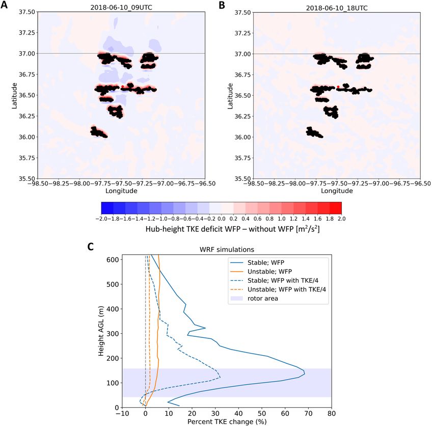
www.nature.com/scientificreports/
Figure 1. Map of the region and the three measurement sites whose observations are considered in the analysis.
The clusters of differently colored dots show wind plants in the region. The named wind plants are those listed in
Table 1 and relevant to this analysis. Map created by the authors using the QGIS v3.10.14 open-source software
(qgis.org). Digital elevation model data courtesy of the US Geological Survey.
models at finer horizontal and vertical resolutions for accurately assessing wind plant impacts. In addition, the
vast array of long-term instrumentation at SGP offers a unique opportunity to compare simulated wind plant
effects with what is seen in real world observations. Therefore, in our analysis, to identify the effects of wakes on
longer-term meteorological conditions at the SGP, we first consult a nine-day simulation of wind plant wakes
using the state-of-the-art Weather Research and Forecasting (WRF) mesoscale model’s30 wind farm parameteri-
zation (WFP)31 to identify the meteorological characteristics of the wake that might be expected from the wind
plants near the ARM facility. Next, we examine observations from ARM instrumentation from 2010 to 2020 to
check for such wake signatures.
Results
Quantifying wind plant impacts on atmospheric conditions. For the observational component of
our analysis, we focus on measurements collected at three sites (see map in Fig. 1): Lamont (C1), Newkirk (E33),
and Omega (E38). At the SGP, southerly winds are the most dominant wind regime, followed by winds flowing
from the north. On the other hand, easterly and westerly winds are extremely rare, as shown in the wind rose in
Fig. 2A, obtained using 8 years of hub-height wind speed observations at the C1 site. Given this wind regime and
the relative distances between measurement sites and nearby wind plants (details are included in Table 1), for
the observational analysis we focus only on assessing the impacts of the southern portion of the Thunder Ranch
wind plant at the C1 site and of Kay Wind at the E33 site. In fact, given the dominant wind regimes, the C1 and
E33 measurement sites are often downwind of these two wind plants, and their relatively short distances from
the closest turbines allows for significant wake effects to be expected at the sites.
To quantify the wind plant impacts using atmospheric observations, we consider 8 years of data collected by
both remote sensing and in situ instruments. At C1, we use 30-min average wind speed measurements from a
Halo Streamline l idar32 from 2012 to 2020. We use three-dimensional sonic anemometers on flux measurement
systems deployed at each of the three considered measurement sites from 2011 to 2019 to measure near-surface
(4 m AGL) wind speed and turbulence kinetic energy (TKE). Also, we use the observed surface-layer fluxes to
quantify atmospheric stability at each site in terms of the Obukhov length, L. The distribution of the considered
stability classes at C1 as a function of hour of day for the full 8-year period is shown in Fig. 2B.
To more generally explore the expected impact of nearby wind plants we use numerical simulations, com-
paring 7 days of WRF simulations at the SGP site with and without a WFP31,33–35. The parameterization has two
impacts. First, it extracts kinetic energy from the mean flow via a drag or momentum sink term in the momentum
equations of WRF, based on the hub-height wind speed. Second, it explicitly adds TKE (to that parameterized
in the MYNN scheme for subgrid fluxes) at the model levels intersecting the wind turbine rotor disk. In our
present analysis, we conduct three sets of simulations, including one with no turbines (without WFP). The two
sets of simulations with turbines include either the original TKE source (WFP) or 25% of the original TKE source
(WFP25), following indications within the scientific debate on the presence and magnitude of the TKE source in
wind plant p arameterizations35–39. We consider the variability of the results between the two parameterization
setups (WFP and WFP25) as a proxy for the uncertainty (especially in TKE changes) resulting from the specifics
Scientific Reports | (2021) 11:22939 | https://doi.org/10.1038/s41598-021-02089-2 2
Vol:.(1234567890)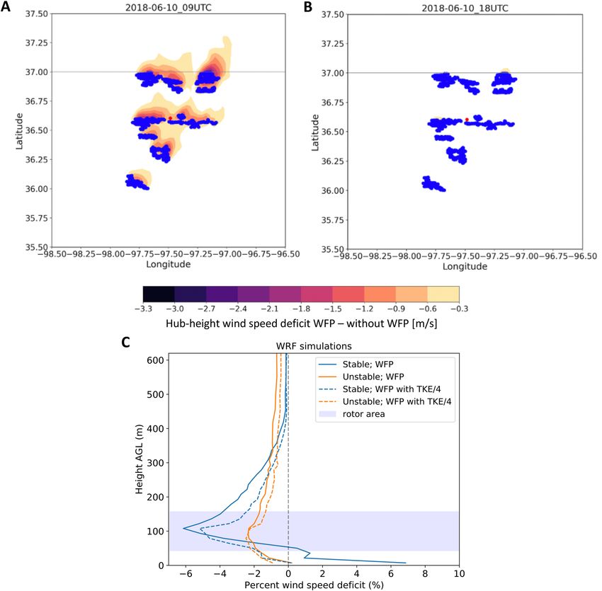
www.nature.com/scientificreports/
Figure 2. (A) 91-m wind rose from the C1 lidar using observations from September 2012 to October 2020.
(B) Histogram of the atmospheric stability conditions (classified in terms of the surface Obukhov length) as a
function of the hour of the day at the C1 site. Data from September 2011 to October 2019.
Distance from
Impacting wind closest turbine Waked wind
Site plant Year built Hub height (m) Rotor diameter (m) (km) direction sector
Thunder Ranch 2017 90 116 3.5 112 ◦–196 ◦
C1—Lamont 6.7 67 ◦–93 ◦
Chisholm View 2012 80 82.5 4.6 243 ◦–270 ◦
Kay Wind 2015 80 108 1.3 252 ◦–23 ◦
E33—Newkirk
Frontier I 2016 87 126 7.1 195 ◦–235 ◦
Canadian Hills 2012 80 102 18.5 –
E38—Omega
Kingfisher Wind 2015 80 100 25.5 –
Table 1. Main characteristics of the wind plants in the vicinity of the sites considered in the analysis.
of the WFP. To this regard, we note how the parameterization proposed by Volker et al.37 is not publicly available,
and therefore a direct comparison of the results between different WFPs was not possible.
Wind plant effects on wind speed. As shown in other simulation studies29,40, the presence of the wind
plant induces a wake that varies with wind speed, wind direction, and ambient turbulence. In the “Supple-
mentary Materials”, we include an animation of how the WRF-modeled wind plant wakes vary throughout the
considered period. Contours of the wake wind speed deficit at two sample times are shown in Fig. 3A,B. The
magnitude of the wake increases as wind speed increases toward the rated wind speed of the turbines; the wake
erodes quickly in daytime convective conditions (Fig. 3B) but persists for long distances downwind in stable
conditions (Fig. 3A). To further validate this qualitative variability, we compute an average vertical profile of the
wind speed deficit at the C1 site in different stability conditions. We calculate the percentage wake wind speed
deficit at the C1 site by first subtracting the results from the simulation with no wind plants from the simulations
with wind plants (either WFP or WFP25), which is then normalized by the results without the WFP. Also, we
select only wind speeds when turbines are expected to be operational (wind speed at ∼ 90 m above ground level
(AGL) between 3 and 25 m s−1) and when wind directions are expected to impose wake impacts from Thunder
Ranch on the C1 site (simulated wind directions between 112◦ and 196◦). To check the effects of atmospheric
stability, we separate data using the sign of the surface heat flux as simulated by WRF at the location of the C1
lidar; we consider stable conditions for negative surface heat flux and unstable conditions for positive surface
heat flux. The median profile of the simulated wake wind speed percentage deficits at the C1 lidar location is
shown in Fig. 3C (the median profile of the actual wind speed deficit is included in the “Supplementary Materi-
als” in Fig. S3). The median profile confirms that at most altitudes, the strongest wakes occur in stable conditions
for both the WFP and WFP25 cases. Near the surface, accelerations occur in stably stratified conditions but only
for the simulations with 100% TKE included. The weaker TKE source (WFP25) shows no accelerations near the
surface. Both simulations show a maximum wind speed deficit in the top half of the wind turbine rotor disk but
with some detectable deficit persisting up to nearly 400 m above the surface. In these simulations, estimates of
stable boundary layer height (not shown) range from 100 to 500 m above the surface. In unstable conditions,
both the WFP and WFP25 simulations exhibit a weaker wind speed deficit than in stable conditions, with the
maximum wind speed deficit near hub height. Although the unstable wind speed deficit is weaker than that of
Scientific Reports | (2021) 11:22939 | https://doi.org/10.1038/s41598-021-02089-2 3
Vol.:(0123456789)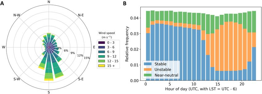
www.nature.com/scientificreports/

                                            Figure 3.  (A, B) Contours of hub-height wind speed deficit calculated by subtracting the simulation without
                                            the WFP from the WFP simulation at two sample times on June 10: (A) 0900 UTC (0300 LT); (B) 1800 UTC
                                            (1200 LT); blue dots represent wind turbines. (c) Median profile of WRF-simulated percentage wind speed
                                            deficit (calculated as either (WFP − without WFP)/(without WFP) or (WFP25 − without WFP)/(without WFP))
                                            at the C1 location for stable (negative surface heat flux) and unstable (positive surface heat flux) conditions for
                                            wind directions between 112◦ and 196◦.

                                            the stable conditions, it is also detectable at higher altitudes, likely caused by convective mixing throughout the
                                            deeper convective boundary layer.
                                               Similar effects emerge from the long-term atmospheric observations. First, we consider measurements aloft
                                            using the lidar measurements at C1 to quantify the impact that the southern portion of the Thunder Ranch
                                            wind plant has on the long-term lidar data. Although the use of numerical simulations allows for the concur-
                                            rent availability of data with and without wind plants, this is obviously not the case when looking at real-world
                                            observations; therefore, to quantify the wind speed deficit, we calculate at each lidar measurement height, z, a
                                            normalized median difference in wind speed between the post- and pre-wind plant periods (pre-wind plant data
                                            include 2012–2016, post-wind plant data include 2018–2020):

          Scientific Reports |   (2021) 11:22939 |               https://doi.org/10.1038/s41598-021-02089-2                                                  4

Vol:.(1234567890)
www.nature.com/scientificreports/
Figure 4. (A) Median wind speed percentage deficit between post- and pre-wind plant periods calculated from
the lidar observations at C1 for stable and unstable conditions. The blue shaded area shows the vertical limits
of the turbine rotor disks (which have been corrected for the < 10-m terrain elevation difference between the
lidar location and the Thunder Ranch wind plant). (B, C) Median percentage change in 4-m wind speed when
comparing post- and pre-wind plant observations as a function of wind direction. Data at C1 are normalized
according to Eq. (2) using observations at E33 (B) and E38 (C). In each panel, the background blue shading
indicates the wind direction distribution.
median(WSpost,z ) − median(WSpre,z )
diffWS,z = (1)
median(WSpre,z )
We consider only cases with observed 90-m wind speeds between 3 and 25 m s−1 and wind directions between
112◦ and 196◦, as explained for the WRF case. Figure 4A shows how the median observed wind speed percentage
deficit varies with height for stable and unstable conditions (actual wind speed deficit shown in Fig. S4a). The
shape of the wake’s vertical profile from the long-term lidar observations generally agrees well with the short-
term WRF simulation results (as shown in Fig. 3C), although with some interesting differences in the profile.
Both observations and WRF simulations confirm that the wake deficit is stronger in stable conditions, and the
magnitude of the observed deficit better agrees with the simulated WFP case than the WFP25 case; however, the
peak of the observed wind speed deficit occurs at higher altitudes than the peak in either of the WRF simula-
tions. In fact, although both the WFP and WFP25 simulations showed a maximum wind speed deficit at hub
height, the lidar observations display a significant lifting of the location of these peaks. In stable conditions,
the altitude of the maximum deficit is near the top of the turbine rotor disk, 75 m above the maximum deficit
in the simulations; in convective conditions, the maximum deficit is lofted ∼ 150 m above the altitude of the
maximum in the simulations. This lofting of the wake in convective conditions is consistent with o bservations41
in complex terrain and should therefore be explored further at the SGP site to assess if terrain effects, perhaps
unresolved by the model simulations, induce this effect. In addition, the long-term observations reveal a strong
acceleration (up to +10%) in both stable and unstable conditions. The near-surface acceleration emerges only in
Scientific Reports | (2021) 11:22939 | https://doi.org/10.1038/s41598-021-02089-2 5
Vol.:(0123456789)www.nature.com/scientificreports/
stable conditions for the WRF simulations with the WFP and not at all in the WFP25 simulations. Further, the
observed accelerations occur at higher altitudes than the WRF results. Accelerations near the surface in wake
regions also occur in large-eddy simulations of wind p lants38. To further explore the near-surface acceleration
caused by the wind plant wake, we compare post- and pre-wind plant wind speeds observed from the 4-m sonic
anemometers deployed at the three measurement sites considered. The existence of concurrent observations at
three locations allows for a further normalization of the wind speed difference to reduce the impact of the wind
resource interannual variability; therefore, for the near-surface observations, we modify Eq. (1) and take the
difference of the observations at the C1 site with data from either E33 or E38, so the normalized wind speed
difference metric becomes (when using E33 for the normalization):
median(WSpost,C1,4m − WSpost,E33,4m ) − median(WSpre,C1,4m − WSpre,E33,4m )
diffWS,4m = (2)
median(WSpre,C1,4m )
In this calculation, pre-wind plant data are from 2011 to 2014 (because the Kay Wind wind plant, near E33,
was built in 2015), and post-wind plant data include 2018 and 2019 (i.e., after both Kay Wind and Thunder Ranch
were built). Figure 4B,C show how diffWS,4m varies as a function of wind direction using both E33 (Fig. 4B) and
E38 (Fig. 4C) for the normalization of the metric. Corresponding plots for the actual (vs percent) changes in
wind speed are shown in the “Supplementary Materials”. In both cases, for the wind direction sector in which
the Thunder Ranch wind plant is upwind at C1 (rose shaded area in both Fig. 4B,C), we see how after the wind
plant was built, the surface wind speed is nearly 10% larger in stable conditions (blue dots), whereas little change
is observed in unstable conditions (orange dots) when strong turbulence quickly erodes wakes. Similarly, when
the E33 site is in the wake of the Kay Wind wind plant (yellow shaded area in Fig. 4B), post-wind plant surface
wind speed increases by more than 10–20% (which appears as negative values in the figure because of how the
normalization was defined in Eq. (2)), whereas no significant changes are observed in unstable conditions. On the
other hand, for wind direction sectors not affected by wind plants (white areas in both panels Fig. 4B,C), no sig-
nificant change in surface wind speed occurs in either stable or unstable conditions in the post-wind plant period.
Wind plant effects on turbulence kinetic energy. TKE is generated by wind turbines as they extract
momentum from the wind flow, so it represents another major impact of wind plants on the local atmospheric
flow. As shown in the WRF-simulated results in Fig. 5A,B, the immediate vicinity of the wind turbines always
exhibits a large positive increase in TKE, but that increase erodes rapidly downwind. In stable conditions
(Fig. 5A), the simulation with wakes shows reduced TKE in far downwind regions, likely because of reduced
wind shear in the WFP simulation, as discussed i n42. To generalize this qualitative impact from the WRF simula-
tions, we follow the same approach used to assess the wind speed deficit, and we calculate the percentage TKE
change at the C1 site by comparing the simulations without wind plants to those with wind plants (WFP and
WFP25). As done for wind speed, we consider only cases where hub-height simulated wind speed is between 3
and 25 m s−1 and when the C1 location is directly downwind of the Thunder Ranch wind plant. Figure 5C shows
the median profile of the WRF-simulated percentage TKE change at C1 (actual TKE change shown in Fig. S5,
along with median TKE profiles in Fig. S6). Maximum TKE enhancements occur at the C1 lidar during stable
conditions. In both WRF WFP setups, the peak TKE change emerges in the upper half of the turbine rotor area.
On the other hand, TKE is only slightly enhanced during unstable conditions, which are already very turbulent
because of surface convective heating. Also, this slight TKE enhancement is more uniform throughout the con-
sidered height range, which is consistent with the increased turbulent mixing in convective conditions. At the
surface, a significant increase in TKE emerges only in stable conditions for the WFP WRF setup.
No long-term observations of TKE at hub height are available at the SGP site. Still, we can compare the WRF
results with the variability in long-term near-surface observations of TKE. Figure 6 shows how 4-m AGL TKE
varies between post- and pre-wind plant regimes as a function of wind direction using the same normalized
difference metric introduced for wind speed in Eq. (2) (actual TKE change is shown in Fig. S7). Panel A nor-
malizes C1 by the E33 differences; panel B normalizes C1 by E38. The range of wind directions in which wind
plant impacts are expected at C1 are highlighted in rose, whereas the range of wind directions in which wind
plant impacts are expected at E33 are highlighted in yellow. In both cases, the surface TKE in stable conditions
(blue dots) is enhanced by 15–30% when wind plants are located upwind of the measurement site (again, we see
negative values in the yellow wind direction sector because of how the normalization was defined in Eq. (2)).
On the other hand, in unstable conditions, few differences are detectable between the post- and pre-wind plant
conditions when wake erosion is significantly faster. Both results are consistent with those found from the WRF
simulations, although the observed increase in surface TKE is greater than what WRF predicts close to the
ground. Finally, for wind directions not directly affected by wind plant wakes (white vertical bands in the plots),
no changes in observed surface TKE between the post- and pre-wind plant regimes can be detected. We note that
we have investigated the variability of upwind terrain elevation at the C1 site for all wind directions (see Fig. S8
in the “Supplement”), and did not find any higher changes in terrain roughness for southerly flow, which could
have also caused the increased near-surface turbulence noticed here.
Discussion
Changing environments can have a significant impact on nearby long-term weather and climate observatories.
In cities and towns, the urban heat island e ffect13,14 is well known to affect local atmospheric conditions. Here,
we assessed the wind plant wake effect on local atmospheric conditions at the U.S. Department of Energy’s ARM
SGP site in northern Oklahoma. Recent increases in wind energy deployment near this and other long-term
Scientific Reports | (2021) 11:22939 | https://doi.org/10.1038/s41598-021-02089-2 6
Vol:.(1234567890)www.nature.com/scientificreports/
Figure 5. (A, B) Contours of the difference in hub-height TKE calculated by subtracting the simulation without
WFP from the WFP simulation at two sample times on June 10: (A) stable conditions, at 0900 UTC (0300
LT); (B) unstable conditions, at 1800 UTC (1200 LT); black dots represent wind turbines. (C) Median profile
of WRF-simulated percentage TKE change (calculated as either (WFP − without WFP)/(without WFP) or
(WFP25 − without WFP)/(without WFP)) at the C1 location for stable (negative surface heat flux) and unstable
(positive surface heat flux) conditions for wind directions between 112◦ and 196◦.
weather and climate observatories suggest that it is critical to quantify the likely impacts of these changes in
effective roughness and mixing on weather and climate observations. Our simulations include a short time
period (7 days) of primarily southerly winds. Our observational record considers data from 2011 to 2020. Both
simulations and observations show that at the ARM SGP C1 site, approximately 3.5 km downwind of a row of
wind turbines, wind speed at wind turbine rotor altitudes decreases by up to 6% in stable conditions, whereas
unstable conditions experience a subtle wind speed deficit, not larger than 2%. Near the surface, both the local
observations and WRF simulations including a 100% TKE source reveal a significant (∼ 10%) acceleration during
stable conditions. At the location of the ARM SGP C1 site, TKE is also highly affected by the presence of wind
plants. In stable conditions, TKE greatly increases in the WRF simulations, with the maximum change near the
top of the turbine rotor disks. Long-term observations confirm this variability, with significant increases (+30%)
in surface TKE in stable conditions and little change in unstable conditions when boundary layer turbulence
values are already large as a result of convection driven by surface heating. Other meteorological parameters can
Scientific Reports | (2021) 11:22939 | https://doi.org/10.1038/s41598-021-02089-2 7
Vol.:(0123456789)www.nature.com/scientificreports/
Figure 6. (A, B) Median percentage change in 4-m TKE when comparing post- and pre-wind plant
observations as a function of wind direction. Data at C1 are normalized according to Eq. (2) (but applied to TKE
instead of wind speed) using observations at E33 (A) and E38 (B). In each panel, the background blue shading
indicates the wind direction distribution.
be influenced by wind plant wakes. Both in situ and satellite observations have suggested that nocturnal surface
temperatures increase in the vicinity of wind plants as wind turbines mix warmer air from aloft down to the
surface. The long-term temperature analysis at this site is complicated by the changing surface cover through
the years available for study, by shifts in the timing of transitions in the boundary layer caused by the presence of
the wind p lants43, as well as by the confounding effects of subtle variations in local t errain44. Subsequent analysis
could explore wind plant wake effects on sensible and latent heat fluxes. Also, a similar analysis could be repli-
cated for different topographic conditions, ranging from offshore to more complex terrain on land.
Methods
Area of analysis. The SGP site is a long-term atmospheric observatory managed by the U.S. Department of
Energy’s ARM research facility in north-central Oklahoma (Fig. 1). The rural region is characterized by relatively
simple topography, and its land use is primarily cattle pasture and wheat fields. The median Terrain Ruggedness
Index45 calculated over the region around the SGP Central Facility using a 1/3 arc-second Digital Elevation
Model is ∼ 0.2 m. Many wind plants have been built in the area in recent years. They are highlighted by the
colored dots in Fig. 1. The C1 site represents the heart of the array of observational equipment at the SGP site,
and it has two wind plants in its vicinity: Thunder Ranch to the south and east (yellow-green dots in Fig. 1) and
Chisholm View to the west (light blue dots in Fig. 1). The E33 site is approximately 35 km northeast of C1, near
the Kay Wind wind plant (salmon dots in the map) and the Frontier I wind plant (blue dots in the map). Finally,
E38, approximately 65 km southwest of C1, is generally unaffected by the wind plants in the region, which are at
least 18 km from the measurement site. Table 1 includes details of the wind plants in the vicinity of the measure-
ment sites, their mutual minimum distance, and the wind direction sectors for which the measurement sites are
downwind of the wind plants.
Observational equipment. At C1, we use wind speed measurements from a Halo Streamline lidar32 from
September 2012 to October 2020. Wind speed data from the lidar are retrieved from the line-of-sight velocity
recorded during the full 360◦ conical scans, which were performed every ∼ 10–15 min and took approximately
1 min each to complete. Wind speed is retrieved using the approach described in46 by assuming horizontal
homogeneity over the scanning volume. Data are then averaged at a 30-min resolution. The instrument operated
with a range gate resolution of 30 m, and the lowest height available was 65 m AGL. We discard from the analysis
measurements with a signal-to-noise ratio less than −21 dB or greater than +5 dB (to filter out fog events, rela-
tively common at SGP), together with periods of precipitation, as recorded by a disdrometer at C1. Additional
technical specifications of the lidar are shown in Table 2.
We use in situ instruments to measure near-surface (4-m AGL) wind speed and TKE. We consider data from
three-dimensional sonic anemometers deployed at each of the three considered measurement sites. The instru-
ments provide measurements at 10-Hz resolution, which are then averaged at 30-min intervals. At all sites, we
use observations from September 2011 to October 2019, the longest period where concurrent measurements
from all three locations are available. TKE is provided as a 30-min average, and it is calculated from the variance
of the three components of the wind flow as
Scientific Reports | (2021) 11:22939 | https://doi.org/10.1038/s41598-021-02089-2 8
Vol:.(1234567890)www.nature.com/scientificreports/
Wavelength 1.5 µm
Laser pulse width 150 ns
Pulse rate 15 kHz
Pulses averaged 20,000
Points per range gate 10
Range-gate resolution 30 m
Minimum range gate 15 m
Number of range gates 200
Table 2. Main technical specifications of the C1 Halo lidar.
1 2
TKE = (σ + σv2 + σw2 ). (3)
2 u
Also, we use surface data to quantify the atmospheric stability at each site in terms of the Obukhov length L:
Tv · u∗3
L=− (4)
k · g · w ′ Tv′
where k = 0.4 is the von Kármán constant; g = 9.81 m s−2 is the gravity acceleration; Tv is the virtual temperature
2 2
(K); u∗ = (u′ w ′ + v ′ w ′ )1/4 is the friction velocity (m s−1); and w ′ Tv′ is the kinematic virtual temperature flux
(K m s−1). A 30-min averaging period is used for the Reynolds decomposition, a common choice for atmospheric
boundary layer calculations47,48. We classify stable conditions for 0 m < L ≤ 200 m (0 < z/L ≤ 0.02), unstable
conditions for −200 m ≤ L < 0 m (−0.02 ≤ L < 0), and near-neutral otherwise. As done for the lidar data, we
discard precipitation periods to remove inaccurate measurements.
Mesoscale model setup. Our simulations use the WRF model49 version 4.2.1 and the WFP31. While hav-
ing long-term WRF simulations at the SGP site would be ideal to match the observational analysis, this is not
computationally feasible; therefore, here we focus on a 9-day period in 2018, June 10–18, chosen because of
the strong and repeated occurrences of nocturnal low-level jets, as seen in the lidar contours of the wind speed
(Fig. S1 in the “Supplement”). We exclude from the analysis June 13–14 because of strong precipitation events
in the region, which could affect the accuracy of the WRF predictions50. Two one-way nested domains (9-km
horizontal resolution with 250 × 250 points and 3-km horizontal resolution with 301 × 301 points) are simu-
lated, with both domains centered at 36.605◦ N, 97.485◦ W, the location of the C1 site. The 58 vertical levels
include eight levels in the lowest 100 m, following best-practice r ecommendations29. Initial and boundary con-
ditions come from the ERA5 reanalysis product51. The Rapid Radiative Transfer Model (RRTM) shortwave and
longwave radiation s chemes52 represent radiative processes, whereas a cumulus parameterization is active only
on the 9-km domain. The planetary boundary layer scheme is the MYNN s cheme53, currently the only scheme
that functions with the WFP. Each of the 9 days is run separately with 24 h of spin-up time to ensure accurate
representation of surface soil moisture54.
To represent the effects of wind turbines, we use the WRF WFP. The original version31 has experienced several
updates and c hanges33–35. The presence and magnitude of the TKE source in the wind plant parameterizations
is an area of scientific debate. Some wind plant parameterizations do not explicitly add T KE36,37 and allow it to
be developed from wind shear caused by the momentum sink. Comparisons to large-eddy s imulations38 and
observations39, however, suggest that the TKE source term is critical to include, although some investigators35
suggest that the TKE source term should be reduced. Further, the integration of the WFP with boundary layer
parameterizations other than the MYNN scheme might support more shear-developed t urbulence55. In our pre-
sent analysis, we conduct three sets of simulations, including one with no turbines. The two sets of simulations
with turbines include either the original TKE source (WFP) or 25% of the original TKE source (WFP25). WRF
namelists and wind turbine supporting files are available at https://doi.org/10.5281/zenodo.4641408.
We include 949 turbines in the simulation; their locations are taken from the US Geological Survey database56,
and each is represented as a 2-MW turbine with 80-m hub height and 80-m rotor diameter. The actual turbines
in this domain all have slightly different capacities (ranging from 1.5 to 2.3 MW), hub heights (ranging from
80 to 90 m), and power curves. Within the WRF simulations, we represent them all with the same power curve
with a 3-m s−1 cut-in speed, 12-m s−1 rated speed, and 25-m s−1 cut-out speed (Fig. S2 in the “Supplement”).
Other researchers12 have investigated the sensitivity of the WFP to exact turbine power curves by varying the
wind turbine thrust and power coefficients by 10%. They found that the uncertainty of the resulting wind speed
deficit induced by these coefficients was smaller than the uncertainty induced by a suite of other physics and
numeric permutations, including a change in the number of vertical levels; thus, we do not use unique turbine
characteristics for the turbines in this region. The turbines included in the simulation setup are shown in Fig. 1,
except for the two wind plants in the vicinity of site E38, which were omitted from the WRF runs because they
do not impact any measurement site. The exact turbine locations are available at https://d oi.o
rg/1 0.5 281/z enodo.
4641408. When multiple turbines are located within a single grid cell, as often occurs, the drag and TKE source
are multiplied by the number of turbines within the cell and integrated over the cell. The amount of drag and
Scientific Reports | (2021) 11:22939 | https://doi.org/10.1038/s41598-021-02089-2 9
Vol.:(0123456789)www.nature.com/scientificreports/
TKE is a function of hub-height wind speed rather than rotor-equivalent wind speed, although an option for
eveloped34.
considering rotor-equivalent wind speed has been d
Data availability
WRF namelists and supporting files required to run the WRF simulations in our analysis are available at https://
doi.org/10.5281/zenodo.4641408. All the observations used in the analysis are publicly available at the follow-
ing DOIs: https://doi.org/10.5439/1025186; https://doi.org/10.5439/1025039; https://doi.org/10.5439/1025036;
https://doi.org/10.5439/1342140.
Received: 12 May 2021; Accepted: 9 November 2021
References
1. Tennekes, H. & Lumley, J. L. A first course in turbulence. MIT press, 1972.
2. Lissaman, P. B. S. Energy effectiveness of arbitrary arrays of wind turbines. J. Energy 3, 323–328. https://doi.org/10.2514/3.62441
(1979).
3. Veers, P. et al. Grand challenges in the science of wind energy. Science 366 (2019).
4. Sørensen, J. N. & Shen, W. Z. Numerical modeling of wind turbine wakes. J. Fluids Eng. 124, 393–399 (2002).
5. Barthelmie, R. J. et al. Modelling and measuring flow and wind turbine wakes in large wind farms offshore. Wind Energy Int. J.
Progress Appl. Wind Power Conv. Technol. 12, 431–444 (2009).
6. Iungo, G. V., Wu, Y.-T. & Porté-Agel, F. Field measurements of wind turbine wakes with lidars. J. Atmos. Ocean. Technol. 30, 274–287
(2013).
7. Machefaux, E. et al. An experimental and numerical study of the atmospheric stability impact on wind turbine wakes. Wind Energy
19, 1785–1805 (2016).
8. Bodini, N., Zardi, D. & Lundquist, J. K. Three-dimensional structure of wind turbine wakes as measured by scanning lidar. Atmos.
Meas. Tech. 10, 2881–2896 (2017).
9. Platis, A. et al. First in situ evidence of wakes in the far field behind offshore wind farms. Sci. Rep. 8, 1–10 (2018).
10. Baidya Roy, S., Pacala, S. W. & Walko, R. Can large wind farms affect local meteorology? J. Geophys. Res. Atmos. 109 D19101 (2004).
11. Rajewski, D. A. et al. Crop wind energy experiment (CWEX): Observations of surface-layer, boundary layer, and mesoscale
interactions with a wind farm. Bull. Am. Meteorol. Soc. 94, 655–672 (2013).
12. Siedersleben, S. K. et al. Micrometeorological impacts of offshore wind farms as seen in observations and simulations. Environ.
Res. Lett. 13, 124012 (2018).
13. Howard, L. The Climate of London, Vol. I–III (London, 1833). http://urban-climate.org/documents/LukeHoward_Climate-of-
London-V1.pdf. Accessed 15 Nov 2021.
14. Oke, T. R. The energetic basis of the urban heat island. Quart. J. Royal Meteorol. Soc. 108, 1–24 (1982).
15. Armstrong, A. et al. Ground-level climate at a peatland wind farm in Scotland is affected by wind turbine operation. Environ. Res.
Lett. 11, 044024 (2016).
16. Peña, A., Réthoré, P.-E. & Rathmann, O. Modeling large offshore wind farms under different atmospheric stability regimes with
the park wake model. Renew. Energy 70, 164–171 (2014).
17. Brower, M. Wind Resource Assessment: A Practical Guide to Developing a Wind Project (Wiley, New York, 2012).
18. Fleming, P. et al. Field test of wake steering at an offshore wind farm. Wind Energy Sci. 2, 229–239 (2017).
19. Phadke, A. 2035: Plummeting Solar, Wind and Battery Costs can Accelerate Our Clean Electricity Future; Goldman School of Public
Policy (University of California Berkeley, Berkeley, 2020).
20. DNV, G. Energy transition outlook 2018: A global, regional forecast of the energy transition to 2050. 17, 2018 (2018) (Last accessed
Dec).
21. Song, J., Liao, K., Coulter, R. L. & Lesht, B. M. Climatology of the low-level jet at the southern great plains atmospheric boundary
layer experiments site. J. Appl. Meteorol. 44, 1593–1606 (2005).
22. Greene, S., McNabb, K., Zwilling, R., Morrissey, M. & Stadler, S. Analysis of vertical wind shear in the southern great plains and
potential impacts on estimation of wind energy production. Int. J. Glob. Energy Issues 32, 191–211 (2009).
23. Bodini, N. & Optis, M. The importance of round-robin validation when assessing machine-learning-based vertical extrapolation
of wind speeds. Wind Energy Sci. 5, 489–501 (2020).
24. Bodini, N. & Optis, M. How accurate is a machine learning-based wind speed extrapolation under a round-robin approach? J.
Phys. Conf. Series. 1618, 062037 (2020). (IOP Publishing).
25. Klein, P. et al. LABLE: A multi-institutional, student-led, atmospheric boundary layer experiment. Bull. Am. Meteorol. Soc. 96,
1743–1764 (2015).
26. Bonin, T. A., Blumberg, W. G., Klein, P. M. & Chilson, P. B. Thermodynamic and turbulence characteristics of the Southern Great
Plains nocturnal boundary layer under differing turbulent regimes. Boundary-Layer Meteorol. 157, 401–420 (2015).
27. Smith, E. N., Gibbs, J. A., Fedorovich, E. & Klein, P. M. WRF model study of the Great Plains low-level jet: Effects of grid spacing
and boundary layer parameterization. J. Appl. Meteorol. Climatol. 57, 2375–2397 (2018).
28. Pielke, R. A. et al. A comprehensive meteorological modeling system—RAMS. Meteorol. Atmos. Phys. 49, 69–91 (1992).
29. Tomaszewski, J. M. & Lundquist, J. K. Simulated wind farm wake sensitivity to configuration choices in the Weather Research and
Forecasting model version 3.8.1. Geosci. Model Dev. 13, 2645–2662 (2020).
30. Skamarock, W. C. et al. A Description of the Advanced Research WRF Version 2, Tech. Rep. (National Center For Atmospheric
Research, 2005).
31. Fitch, A. C. et al. Local and mesoscale impacts of wind farms as parameterized in a mesoscale NWP model. Mon. Weather Rev.
140, 3017–3038 (2012).
32. Newsom, R. K. & Krishnamurthy, R. Doppler Lidar (DL) Instrument Handbook (2020). https://www.arm.gov/publications/tech_
reports/handbooks/dl_handbook.pdf. Accessed 15 Nov 2021.
33. Jiménez, P. A., Navarro, J., Palomares, A. M. & Dudhia, J. Mesoscale modeling of offshore wind turbine wakes at the wind farm
resolving scale: A composite-based analysis with the Weather Research and Forecasting model over Horns Rev. Wind Energy. 18,
559–566 (2015).
34. Redfern, S., Olson, J. B., Lundquist, J. K. & Clack, C. T. M. Incorporation of the rotor-equivalent wind speed into the weather
research and forecasting model’s wind farm parameterization. Mon. Weather Rev. 147, 1029–1046 (2019).
35. Archer, C. L., Wu, S., Ma, Y. & Jiménez, P. A. Two corrections for turbulent kinetic energy generated by wind farms in the WRF
model. Mon. Weather Rev. 148, 4823–4835 (2020).
36. Jacobson, M. Z. & Archer, C. L. Saturation wind power potential and its implications for wind energy. Proc. Natl. Acad. Sci. 109,
15679–15684 (2012).
Scientific Reports | (2021) 11:22939 | https://doi.org/10.1038/s41598-021-02089-2 10
Vol:.(1234567890)www.nature.com/scientificreports/
37. Volker, P. J. H., Badger, J., Hahmann, A. N. & Ott, S. The explicit wake parametrisation V1.0: A wind farm parametrisation in the
mesoscale model WRF. Geosci. Model Dev. 8, 3715–3731 (2015).
38. Vanderwende, B. J., Kosović, B., Lundquist, J. K. & Mirocha, J. D. Simulating effects of a wind-turbine array using LES and RANS.
J. Adv. Model. Earth Syst. 8, 1376–1390 (2016).
39. Siedersleben, S. K. et al. Observed and simulated turbulent kinetic energy (WRF 3.8.1) overlarge offshore wind farms. Geosci.
Model Dev. (2020). https://www.geosci-model-dev-discuss.net/gmd-2019-100/. Accessed 15 Nov 2021.
40. Lundquist, J., DuVivier, K., Kaffine, D. & Tomaszewski, J. Costs and consequences of wind turbine wake effects arising from
uncoordinated wind energy development. Nat. Energy 4, 26–34 (2019).
41. Menke, R., Vasiljević, N., Hansen, K. S., Hahmann, A. N. & Mann, J. Does the wind turbine wake follow the topography? A multi-
lidar study in complex terrain. Wind Energy Sci. 3, 681–691 (2018).
42. Xia, G., Zhou, L., Minder, J. R., Fovell, R. G. & Jimenez, P. A. Simulating impacts of real-world wind farms on land surface tem-
perature using the WRF model: Physical mechanisms. Clim. Dyn. 53, 1723–1739. https://doi.org/10.1007/s00382-019-04725-0
(2019).
43. Lee, J. C. Y. & Julie, K. L. Observing and simulating wind-turbine wakes during the evening transition. Boundary-Layer Meteorol
164(3), 449–474 (2017).
44. Acevedo, O. C. & David, R. F. The early evening surface-layer transition: Temporal and spatial variability. J Atmos Sci. 58(17),
2650–2667 (2001).
45. Riley, S. J., DeGloria, S. D. & Elliot, R. Index that quantifies topographic heterogeneity. Intermountain J. Sci. 5, 23–27 (1999).
46. Frehlich, R., Meillier, Y., Jensen, M. L., Balsley, B. & Sharman, R. Measurements of boundary layer profiles in an urban environ-
ment. J. Appl. Meteorol. Climatol. 45, 821–837 (2006).
47. De Franceschi, M. & Zardi, D. Evaluation of cut-off frequency and correction of filter-induced phase lag and attenuation in Eddy
covariance analysis of turbulence data. Boundary-Layer Meteorol. 108, 289–303 (2003).
48. Babic, K., Bencetic Klaic, Z. & Vecenaj, Ž. Determining a turbulence averaging time scale by Fourier analysis for the nocturnal
boundary layer. Geofizika. 29, 35–51 (2012).
49. Skamarock, W. C. et al. A description of the advanced research WRF model version. NCAR Technical Notes 4, 162 (2019).
50. Ancell, B. C., Bogusz, A., Lauridsen, M. J. & Nauert, C. J. Seeding chaos: The dire consequences of numerical noise in NWP per-
turbation experiments. Bull. Am. Meteorol. Soc. 99, 615–628 (2018).
51. Hersbach, H. et al. The ERA5 global reanalysis. Quart. J. Royal Meteorol. Soc. 146, 1999–2049 (2020).
52. Mlawer, E. J., Taubman, S. J., Brown, P. D., Iacono, M. J. & Clough, S. A. Radiative transfer for inhomogeneous atmospheres: RRTM,
a validated correlated-k model for the longwave. J. Geophys. Res. Atmos. 102, 16663–16682 (1997).
53. Nakanishi, M. & Niino, H. An improved Mellor-Yamada level-3 model: Its numerical stability and application to a regional predic-
tion of advection fog. Boundary-Layer Meteorol. 119, 397–407 (2006).
54. Xia, G. et al. Simulating impacts of real-world wind farms on land surface temperature using the WRF model: Validation with
observations. Mon. Weather Rev. 145, 4813–4836 (2017).
55. Rybchuk, A. et al. Integration of a 3D planetary boundary layer scheme and the Fitch Wind Farm Parameterization (2021). in
Wind Energy Science 2021 Conference.
56. Rand, J. T. et al. A continuously updated, geospatially rectified database of utility-scale wind turbines in the United States. Sci.
Data 7, 1–12 (2020).
Acknowledgements
This work was authored in part by the National Renewable Energy Laboratory, operated by Alliance for Sus-
tainable Energy, LLC, for the US Department of Energy (DOE) under Contract No. DE-AC36-08GO28308.
Funding provided by the US Department of Energy Office of Energy Efficiency and Renewable Energy Wind
Energy Technologies Office. The views expressed in the article do not necessarily represent the views of the DOE
or the US Government. The US Government retains and the publisher, by accepting the article for publication,
acknowledges that the US Government retains a nonexclusive, paid-up, irrevocable, worldwide license to publish
or reproduce the published form of this work, or allow others to do so, for US Government purposes.
Author contributions
N.B.: Conceptualization, Methodology, Formal analysis, Writing— Original Draft, Visualization. J.K.L.: Con-
ceptualization, Methodology, Formal analysis, Writing—Original Draft, Visualization. P.M.: Conceptualization,
Writing—Review and Editing, Project administration, Funding acquisition.
Competing interests
The authors declare no competing interests.
Additional information
Supplementary Information The online version contains supplementary material available at https://doi.org/
10.1038/s41598-021-02089-2.
Correspondence and requests for materials should be addressed to N.B.
Reprints and permissions information is available at www.nature.com/reprints.
Publisher’s note Springer Nature remains neutral with regard to jurisdictional claims in published maps and
institutional affiliations.
Scientific Reports | (2021) 11:22939 | https://doi.org/10.1038/s41598-021-02089-2 11
Vol.:(0123456789)www.nature.com/scientificreports/
Open Access This article is licensed under a Creative Commons Attribution 4.0 International
License, which permits use, sharing, adaptation, distribution and reproduction in any medium or
format, as long as you give appropriate credit to the original author(s) and the source, provide a link to the
Creative Commons licence, and indicate if changes were made. The images or other third party material in this
article are included in the article’s Creative Commons licence, unless indicated otherwise in a credit line to the
material. If material is not included in the article’s Creative Commons licence and your intended use is not
permitted by statutory regulation or exceeds the permitted use, you will need to obtain permission directly from
the copyright holder. To view a copy of this licence, visit http://creativecommons.org/licenses/by/4.0/.
© The Author(s) 2021
Scientific Reports | (2021) 11:22939 | https://doi.org/10.1038/s41598-021-02089-2 12
Vol:.(1234567890)You can also read