Symmetry break in the eight bubble compaction - AIMS Press
←
→
Page content transcription
If your browser does not render page correctly, please read the page content below
Mathematics in Engineering, 4(2): 1–24.
                                                                     DOI:10.3934/mine.2022010
                                                                     Received: 25 February 2021
                                                                     Accepted: 17 May 2021
    http://www.aimspress.com/journal/mine                            Published: 15 June 2021

Research article
Symmetry break in the eight bubble compaction†

Giulia Bevilacqua ∗

MOX – Politecnico di Milano, Piazza Leonardo da Vinci 32, Milano, Italy
†
     This contribution is part of the Special Issue: Fluid instabilities, waves and non-equilibrium
     dynamics of interacting particles
     Guest Editors: Roberta Bianchini; Chiara Saffirio
     Link: www.aimspress.com/mine/article/5859/special-articles

* Correspondence: Email: giulia.bevilacqua1993@gmail.com.

Abstract: Geometry and mechanics have both a relevant role in determining the three-dimensional
packing of 8 bubbles displayed in a similar foam structure. We assume that the spatial arrangement of
bubbles obeys a geometrical principle maximizing the minimum mutual distance between the bubble
centroids. The compacted structure is then obtained by radially packing the bubbles under constraint
of volume conservation. We generate a polygonal tiling on the central sphere and peripheral bubbles
with both flat and curved interfaces. We verify that the obtained polyhedra is optimal under suitable
physical criteria. Finally, we enforce the mechanical balance imposing the constraint of conservation
of volume.We find an anisotropy in the distribution of the field of forces: surface tensions of bubble-
bubble interfaces with normal oriented in the circumferential direction of bubbles aggregate are larger
than the ones with normal unit vector pointing radially out of the aggregate. We suggest that this
mechanical cue is key for the symmetry break of this bubbles configuration.
Keywords: symmetry break; optimal tessellation; hepthaedron; mechanical balance; anisotropy

1. Introduction

   Often used for children’s enjoyment, soap bubbles are the simplest physical example of a lot of
mathematical problems. They are solutions of the minimal surface problem [1]: the connection
between soap films and minimal surfaces was established by Gauss in 1830. Indeed, working on
capillarity problems, he found that at equilibrium any liquid surface minimizes the potential energy
caused by molecular forces. In the specific case of soap films, such a energy is proportional to the
area. Hence, soap films are nothing but the physical representation of stable minimal surfaces. Then,
soap bubbles are used to study two dimensional hydrodynamics and turbulence [2]: their use is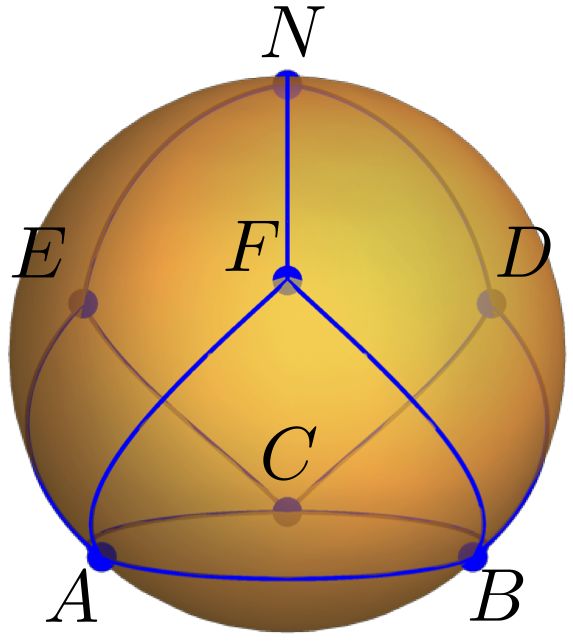
2

motivated by the fact that atmospheric turbulence at large scales displays two dimensional features
due to the small thickness of the Earth’s atmosphere [3]. Indeed, to mimic the emergence of
hurricanes or cyclones in the atmosphere [4], which are the manifestation of turbulence, a half bubble
is heated at the equator giving rise to thermal convection which leads, under some physical
conditions, the appearance of the searched long lived isolated vortices [5]. Finally, they solve an
optimization problem [6]: when two or more bubbles cluster together, their configuration obeys some
physical optimization rules. Indeed, assembling several bubbles traps pockets of gas in a liquid and
results in foam: the surfactants added to the liquid stabilize the bubbles by reducing the surface
tension and by arranging themselves at the liquid/gas interfaces [7].
    Regarding the behavior of a single soap bubble, everything is known. What is not completely
understood is the geometrical and mechanical properties of a cluster of many bubbles, known as a
foam. For instance, its optimal rearrangement in space is still matter of debate.
    In 2D there are more results: Hales proved the honeycomb conjecture, which states that the partition
of the plane into regular hexagons of equal area has least perimeter, i.e., it minimizes the perimeter
fixing the area [8]. In this context, it has been proved that the optimal ( i.e., minimal) configuration
exists for N clusters [9, 10] and Cox et al., obtained their numerical visualizations up to N = 200 [11].
Due to the non linearity of the problem, in a lot of physical situations, the equilibrium solution is only
stable with respect to small displacements, i.e., it is not a global minimum of the system. This aspect
leads to mechanical instabilities which break the symmetry of the system [12–14]. These instabilities
should be classified into two groups [15]: the first one is primarily due to the presence of an asymmetry
in the system and it can be studied though a purely static model. For the second one, the system jumps
away from this initial configuration to settle in another which is not close to it and its description
may require a dynamic model. Just to mention some famous instabilities, we recall the T 1 process in
2-dimension [16], and the 2D flower cluster [13].
    If we move to 3D, the problem is minimizing the area functional and few exact result exist. The
only rigorous one is the proof of the Double Bubble Conjecture [17], which states that the standard
double bubble provides the least-area enclose and separates two regions of prescribed volume in R3 .
As regarding the numerical results, Kelvin [18] proposed an optimal candidate structure with identical
cells, which has been numerically refuted in [19]: by numerical calculations, an agglomerate of two
different types of bubbles has less perimeter, for fixed area.
    The aim of this work is to study the symmetry break of a eight bubble compaction in 3D, i.e., we
want to investigate the mechanical cues driving the three-dimensional packing of 8 bubbles displayed in
a recalling foam structure. To circumvent the difficulty of a variational approach, i.e., the minimization
of an area functional satisfying some geometrical constraints, we follow a different strategy. First of all,
in Section 2, we fix the geometrical arrangement of the eight bubbles as the solution of the Tammes’
problem [20]: we exploit a geometrical principle of maximal mutual distance between neighbor points
on a spherical surface obtaining seven symmetrical peripheral spheres tangent to the central one [21].
Then, compaction is produced by packing the outer bubbles along the radial direction of the aggregate.
The obtained agglomerate recalls the foam structure [22]: the central sphere is completely covered,
while the peripheral ones have a free-curved surface. While our construction does not ensure that
the obtained final configuration is the minimal one, we will prove that the our tessellation on the
central sphere is the optimal one among all the possible [23] according to physical assumptions: the
liquid/liquid interface is favored versus the liquid/gas one and it maximizes the volume [7]. Fixing

Mathematics in Engineering                                                           Volume 4, Issue 2, 1–24.
3
the geometrical arrangement, in Section 3, we look for the balance of forces that produces such a
configuration [6]. Enforcing the mechanical equilibrium and the conservation of volume, we derive
the tensional balance laws on this geometrically optimal packing. Finally, in Section 4, we discuss the
results and we add few concluding remarks.
2. Geometrical principle
2.1. Spatial arrangement
In this section, we introduce a geometrical principle that we exploit to describe the spatial
arrangement of the 8-bubbles configuration, to determine the position of the seven bubbles
surrounding the central one. The coordinates of the peripheral bubbles centroids are given as solution
of the classical Tammes’s Problem [20]: determine the arrangement of n points on the surface of a
sphere maximizing the minimum distance between nearest points (maxmin principle). This is
equivalent to determine (up to rigid rotations) the n unit vectors {ri } such that
( )
1
lim : 1≤i< j≤n , (2.1)
m→+∞ |ri − r j |m
is maximum, where the limit m → +∞ selects the distance among closest points only.
In our case n = 7; we want to find the position of seven points on a sphere with minimum distance
from their nearest neighbors.
Here, we exploit the graph theory [24] to find this maximizing configuration. A set of n points on
a sphere forms a graph G of n points connected by arcs of great circles of length a [25]. The maximal
spatial arrangement of seven points can be obtained by the projective argument presented in [25].
Consider a frame of reference centered in O = (0, 0, 0) and the coordinates on the spherical surface
(r, θ, φ), where θ ∈ [0, 2π) (longitude) and φ ∈ [0, π] (latitude) on S 2 , namely
S 2 = {r, 0 ≤ θ < 2π, 0 ≤ φ ≤ π},
where r is the radius of the sphere N and S the North and South Pole, respectively. Three points
{A, B, C} are placed at the same latitude on the surface of the central sphere, such that they are connected
by arcs of length a and they form an equilateral triangle centered in S , see the triangle ABC d with in
Figure 1a. Three more identical triangles are then created, adjacent to the former ones, with vertices
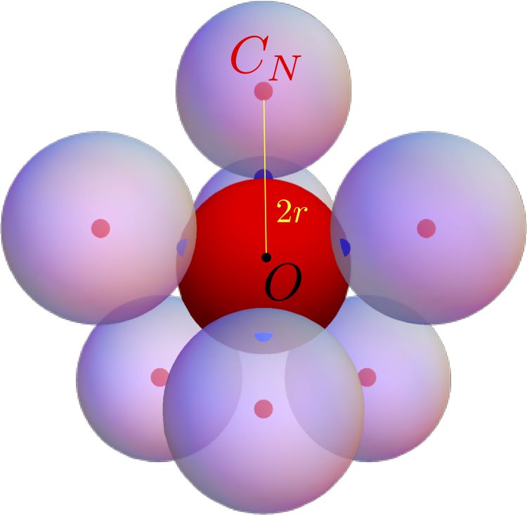
D, E and F: they share the same latitude too, see the triangle ABF d in Figure 1b. The final step is then
to connect D, E and F with N and vary the radius r (for fixed a) until also the latter arcs have length
a∗ , (see Figures 1c and 2). The associated extremal graph defines four triangles and three quadrangles
on the spherical surface, as illustrated in Figure 3.
∗
In a fully equivalent way, one can fix the radius r and vary the chord length a.
Mathematics in Engineering Volume 4, Issue 2, 1–24.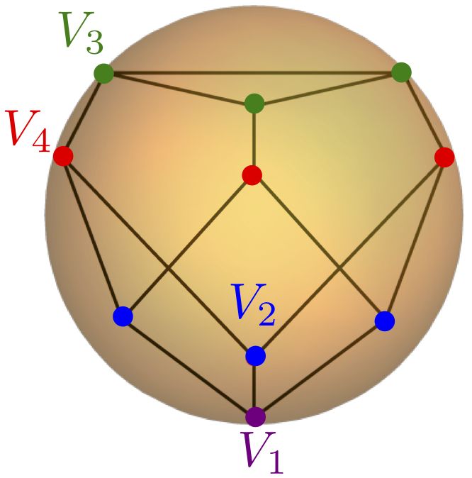
4

        (a) Place {A, B, C}                   (b) Place {D, E, F}         (c) Place {N}
     Figure 1. Steps of Tammes’ construction. (a) First, we place the three points {A, B, C}
                                          d (b) then we place {D, E, F} obtaining three other
     constructing an equilateral triangle ABC,
     triangles like ABF,
                    d and finally (c) we place the North pole N adapting the radius of the
     sphere.

                              (a) Top view                          (b) Side view
     Figure 2. (a) Top and (b) side view of the position and connections of the seven points on the
     spherical surface of the central bubble. The blue connections are the arcs of length a defined
     by Tammes’ construction.

               (a) Stereographic projection                         (b) Spherical projection

     Figure 3. Stereographic (a) and spherical (b) projections of the Tammes’ points on the
     spherical surface and their connecting arcs. Grey and thin lines, corresponding to arcs of
     length 1.34 a, making the tessellation fully triangular.

Mathematics in Engineering                                                           Volume 4, Issue 2, 1–24.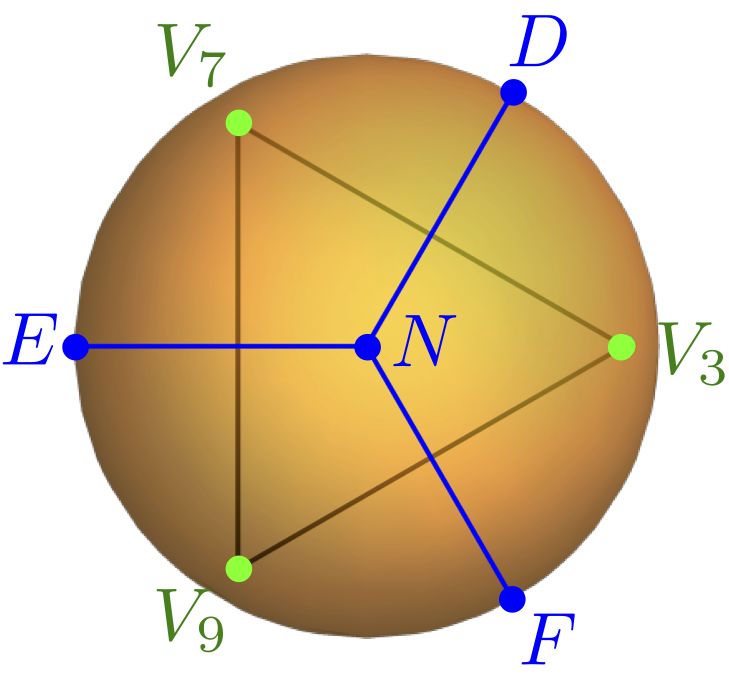
5

   Fundamental relations of spherical trigonometry tell us that the internal angle of an equilateral
spherical triangle is α = 4π
                           9
                             , while the arc angle β with respect to the centre of the sphere β is given
by [26]
                                                     cos 4π
                                           cos β =        9
                                                              ,                                     (2.2)
                                                   1 − cos 4π
                                                            9

as illustrated in Figure 4.

     Figure 4. Geometrical sketch of the latitude of the points A, B and C: the central angle β,
     the radius r of the sphere and the radius rφ of the circumference laying in the plane defined
     by the triplet of points A, B, C.

   This allows to find explicitly the linear relation between arc length and radius, i.e., a = βr. The
length ` of the chord between closest points is
                                                        β
                                             ` = 2r sin     .
                                                         2

2.2. Coordinates
    By construction, the spherical distance on S 2 of the points D, E and F from N is equal to a, so their
latitude is the angle φ pqr = β. For the triplet of points {A, B, C}, the calculations are a little bit more
elaborated. Let rφ be the radius of the circumference defined by the intersection of the sphere and the
plane where A, B and C are. The following relation holds

                                             rφ = r sin (φabc ) ,                                       (2.3)

where φabc is the latitude of the points A, B and C.
Since the chord length is the same for the spherical arc and for the in–plane circle, we find

                                      `                          β
                                                       !
                                                  1 2π
                                         = rφ sin        = r sin     .                                  (2.4)
                                      2           2 3             2

By combining Eqs. (2.3) and (2.4) we get

                                                       2     β
                                          sin φabc   = √ sin     .                                      (2.5)
                                                        3     2

Mathematics in Engineering                                                           Volume 4, Issue 2, 1–24.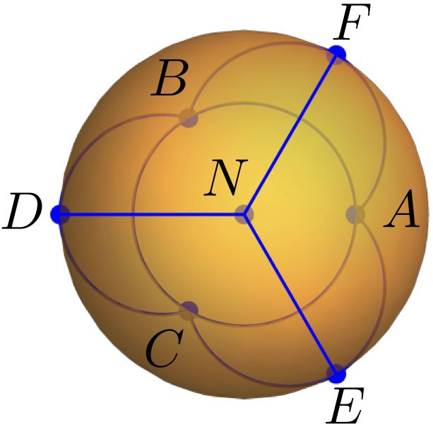
6

Summarizing, the coordinates of the seven Tammes points depicted in Fig. 2 are
                                                             !                   !
                                                     2π                   4π
                         A = (r, 0, φabc )     B = r, , φabc     C = r, , φabc ,
                                                      3                    3
                                                                                                     (2.6)
                   π
                                                                    !
                                                          5π
           D = (r, , φ pqr )     E = r, π, φ pqr     F = r, , φ pqr      N = (r, 0, 0).
                   3                                         3
   This configuration, given by the maxmin principle (2.1), is here adopted as the ideal reference
bubble arrangement: seven spheres are tangent to the former one in the Tammes’ points, as illustrated
in Figure 5a.

                 (a) Before compaction
                                                                   (b) Compaction process
     Figure 5. (a) Initial arrangement of the bubbles before compaction. Tangent points are
     denoted by a blue dot, red dots denote the center of each sphere. (b) Sketch of the
     “compaction process” between two bubbles driven by the parameter δ.

2.3. “Bubble compaction”: tiling the central sphere
   The tessellation of the spherical surface illustrated in the previous sections, is composed by four
equilateral triangles and three quadrilaterals, see Figure 3a. However it can be made of triangles only
by connecting points {D, E, F}, see Figure 3b. The triangle {D, E, N} is not equilateral, since the
distance between D and E is equal to 1.34 a. On the basis of such a triangular tessellation we can
produce a dual tessellation connecting the circumcenters of the triangles: the locus where the axis of
the edges cross each other (Figure 6).
   The Tammes’ points are the centroids of the polygons that define the dual tessellation (see Figure 6
and for more mathematical details Appendix A). The bubble packing is obtained ideally moving each
peripheral bubble, initially tangent to the central one in the Tammes’ points, towards the origin O
along the radial direction, as illustrated in Figure 5b, while enforcing the volume conservation. In
other words, to pack the bubbles aggregate we generate a collection of flat surfaces of contact among
bubbles starting from the maxmin distribution of the tangent points: each peripheral bubble adheres
to the central one moving centripetally, see Figure 5b. At the same time we shuffle the peripheral
and the central spheres to preserve the initial volume V. The contact surfaces between central and

Mathematics in Engineering                                                        Volume 4, Issue 2, 1–24.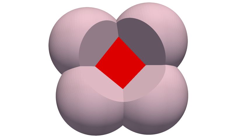
7

peripheral bubbles obtained by such a dive and shuffle procedure are nothing but the polygons obtained
connecting the points of the dual tessellation defined above.

                    (a) Bottom view                                       (b) Top view

     Figure 6. (a) Bottom view of the construction of the dual tessellation. (b) Top view of the
     construction of the dual tessellation.

    The final configuration is a tiling of the spherical surface of the central bubble with seven polygons,
as illustrated in Figure 7:
   • an equilateral triangle centered in N (area ' 0.66 a2 ),
   • three quadrilaterals centered in A, B, C (area ' 0.7 a2 ),
   • three pentagons centered in D, E, F (area ' 0.74 a2 ).

               (a) Stereographic projection                           (b) Independente nodes
     Figure 7. (a) Stereographic projection of the dual tassellation. (b) Sketch of four independent
     nodes V1 , V2 , V3 and V4 on the tessellation, highlighting the corresponding symmetry group.

2.4. Geometrical optimality
   While the produced polygonal surface covers the central sphere, it naturally arises the question if
such a tiling is optimal according to some suitable criterion. The problem to cover a spherical surface

Mathematics in Engineering                                                           Volume 4, Issue 2, 1–24.
8

with polygons is old, rigorous results dating back to Cauchy [27]. In the present context, all the bubbles
are identical and it is therefore tempting the idea to cover the central bubble with identical polygons.
Unfortunately, this is not allowed by Euler’s Polyhedron Formula† .
   There is no regular heptahedron. In order to prove if our tiling is optimal, we can construct all the
convex polyhedra with 7 faces which can be inscribed into a sphere of fixed radius r. By the software
Plantri [23], we find 34 convex polytopes with seven faces. They can be classified in terms of number
of edges and number of vertices, see Table 1.

      Table 1. Classification of the 34 convex polytopes with respect to the number of vertices
      (from left to right) or in terms of edges (from right to left).
                  Number of vertices                   Number of polyhedra                    Number of edges
                  6                                    2                                      11
                  7                                    8                                      12
                  8                                    11                                     13
                  9                                    8                                      14
                  10                                   5                                      15

   In general, an optimal packing rearrangement of soap bubbles is the one which saves energy, i.e.,
we expect the chosen one is the equilibrium configuration which should minimize a suitable assigned
energy functional. However, due to the huge number of variables involved, we are not able to write
down such a functional, hence we use some geometrical and physical considerations to deduce the
optimality and maybe the minimality of the obtained configuration.
   From a physical point of view, it is known that creating an interface liquid/liquid energetically
costs less than one liquid/air [7]. Since the number of edges represents the intersection between
nearest bubbles placed on the Tammes’ points which creates a liquid/liquid interface, maximizing this
number implies that we are requiring that the final polytope on the central sphere has more
liquid/liquid intersections then liquid/air ones, i.e., we are looking for a polyhedron P
                                                                                        e such that

                                                      15
                                                 e = max
                                                 P       EPi          i = 1, ..., 34,                                            (2.7)
                                                        E=11

where EPi is the number of edges the i-polyhedron. In this way, we can reduce the number of polyhedra:
we pass from 34 convex polytopes with 7 faces to just 5 in which our tiling is included. In Appendix
B, we show these 5 polyhedra obtained and drawn by the software Plantri.
   We need another condition to select just one configuration. Using the fact that the shape of a single
soap bubble is spherical, which easily derives from the isoperimetric inequality, i.e., the sphere is the
only solid that, fixing the area, it maximizes the volume, we search among the five configurations
    †
      Euler’s Polyhedron Formula has been proved by Cauchy [27] and it gives a relation among the number of faces, edges and vertices
of a polyhedron, such as
                                                         F + V − E = 2.
The number of vertices and edges are related with the number of faces faces F as follows

                                                          Fn           2E   Fn
                                                     E=           V=      =    ,
                                                          2            m    m
where n is the number of edges of the polygon at hand, while m is the number of faces which insist on the same vertex. We are interested
in the case F = 7. By elementary calculations one can easily see that there is no n for which a suitable integer m exists.

Mathematics in Engineering                                                                                 Volume 4, Issue 2, 1–24.
9

obtained by Plantri, the one that has the maximum volume, indeed we look for a polyhedron P such
that
                                               5
                                          P = max L3 (P
                                                      ei ) ,                                (2.8)
                                                              i=1

where L3 is the volume measure. By numerically computing the five volumes, we find that the tiling
obtained as the dual of the Tammes’ one is the one with maximum volume, i.e., the optimal one
according to our criteria.
Remark 1. Since each polyhedron is not regular, we do not have an explicit formula to compute the
volume. However, each polyhedron can be divided into 7 pyramids, where the basis is a face. Using this
geometrical argument, the total volume can be computed as the sum of the volumes of the pyramids.

2.5. Surfaces, edges and vertices
   The dual tessellation defines ten nodes and it belongs to C3z (1, 3, 3, 3), see Figure 7b‡ . We denote
the nodes of the dual tessellation on the basis of the vertices of the Tammes’ triangles they belong to,
such as
                          V1 = (A, B, C),
                                 V2 = (A, F, B),        V3 = (E, F, N),         V4 = (A, E, F),
                                 V5 = (A, E, C),         V6 = (B, D, C),         V7 = (D, E, N),
                                 V8 = (B, D, E),         V9 = (D, F, N),         V10 = (B, D, F).
Because of the symmetry of the problem, there are only four independent nodes, as depicted in Figure
7b.
    The dual tessellation is formed by 15 edges, only 4 of them being independent. Each edge is
identified by the polygons it belongs to on the tiled surface and the boldface denotes the unit vector
parallel to the edge. Therefore, c1 = V1 V2 denotes the edge between two quadrilaterals, c2 = V2 V3
separates a quadrilateral and a pentagon, c3 = V3 V4 separates a pentagon and a pentagon and c4 = V2 V3
is between a pentagon and the triangle.
    We generate a three dimensional structure projecting radially the dual tessellation, by an height
to be fixed later on the basis of volume conservation arguments. Each vertex of the tessellation on
the central bubble has therefore a corresponding outer one that we denote by Vih , i = 1, 2, 3, 4. The
connection between inner, outer and side surfaces is defined by two classes of edges:

   • c5 = V1 V1h , c6 = V2 V2h , c7 = V3 V3h , c8 = V4 V4h point radially,
   • c9 = V1h V2h , c10 = V2h V3h , c11 = V3h V4h , c12 = V2h V3h , are parallel to the ones on the tessellation of the
     central bubble.
At this stage the geometrical characterization of the 8-bubbles configuration derived on the basis of a
maximum-minimum distance of the centroids of the peripheral bubbles is completed. The inner bubble
has no free surface: it is surrounded by contact interfaces with other bubbles only. The external ones
have the shape of a pyramidal frustum covered by a laterally cut spherical cap: the lower basis is the
polygon generated by the adhesion with the central bubble, lateral sides are flat too, their edges being
   ‡
     Cnz is the group of a cyclic symmetry after a rotation 2π/n with respect to the axis z [28, 29]: the configuration is invariant for
rotations of an angle 2π/3 around the z axis. The notation (1, 3, 3, 3) denotes how many nodes of the tessellation share the same
longitude.

Mathematics in Engineering                                                                                 Volume 4, Issue 2, 1–24.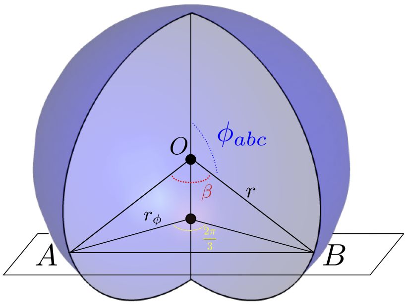
10

radially oriented, the upper basis of the frustum is a radial projection of the lower one. The upper
geometrical structure is a spherical vault on a polygonal frustum, intriguingly known since the Middle
Age in Sicilian architecture [30]. The radius of the spherical cap and the height of the frustum are to
specified on the basis of balance and conservation arguments discussed below.

3. Mechanical balance

   In this section, we compute the surface tensions that make the geometrical packing mechanically
equilibrated. We remark that the central sphere has only bubble–bubble contact interfaces, while the
peripheral ones also possess a traction–free surface. Each bubble–bubble interface and each free
surface is characterized by a tension τi , defined as the energy density per unit area of the liquid/liquid
or liquid/air interfaces [31]. Thus, for the strong symmetry of the problem, we have ten unknown
independent tensions τi , one variable for each portion of surface. Precisely, they are: three on the
central bubble, four on lateral bubble-bubble interfaces and three at the free surface denoted by

                                                   τQ , τP , τT , τQQ , τPQ , τPP , τPT , τQs , τPs , τTs ,                                (3.1)

where the subscript identifies the surface of the polygon it applies to and the superscript s specifies the
tensions at the free surfaces.

3.1. Tensional balance
    First, we enforce the mechanical equilibrium imposing that the surface tensions are balanced on
each independent edge ci , where i = 1, ..., 12 (see Figure 8a). Three (flat or curved) surfaces are
attached to each edge, their local orientation being denoted by the normal unit vectors nij , j = 1, 2, 3.
The balance of tensions on each edge is defined by the sum of the tensions, oriented orthogonally to
the edge and in-plane with the corresponding interface (see Figure 8a). Therefore it must hold
          3
          X                 3
                            X                               3
                                                            X                                     3
                                                                                                  X
                 t jτ j =         ci ×   nij τ j   = ci ×         nij τ j   =0         ⇒                nij τ j = 0 i = 1, ...., 12        (3.2)
           j=1              j=1                             j=1                                   j=1

Equation (3.2) defines 36 scalar equations, 12 of them being trivially null because all the summed
vectors are in the plane orthogonal to the edge under consideration. With the help of a symbolic
software§ , we eventually find that, given the unit vectors nij only 10 of them are independent¶ . The
equations are detailed in Appendix D in Tables 2–4.
   The linear system Eq (3.2) is however not closed because, while the direction orthogonal to the flat
surfaces is uniquely defined, the edge contribution of the tension defined on the free surface depends
on the curvature of the surface itself. Curvature, tension and pressure gap on the free surface of the
peripheral bubbles obey the Young-Laplace equation [32] in the following way

                                                                            4τis
                                                              ∆p =                 i = P, Q, T,                                            (3.3)
                                                                            Ri
   §
     We used Mathematica (Wolfram Inc., Version 12).
   ¶
     The orientation of the normal unit vectors is not defined according any specific rule because it is expected to affect only the sign of
tension, that we know to be positive.

Mathematics in Engineering                                                                                              Volume 4, Issue 2, 1–24.
11
where Ri is the radius of curvature of the free surface of the i-th bubble and ∆p is the difference
between the outer and the inner of pressure and there is an extra factor 2 since the surface of the
bubble is composed by two leaflets. Since we have only three independent types of polygons on the
tessellation, Eq (3.3) gives three independent equations.
(a) Balance on a edge
(b) Volume of a peripheral sphere
Figure 8. (a) Balance of tensions on an edge. (b) The bubble volume is the sum of a
pyramidal frustum (with pink side boundaries) plus the polygonal–basis vault standing on
it (light pink).
3.2. Volume conservation
Finally, we have to impose the conservation of bubble volume under compaction. While the central
(packed) bubble is bounded by flat interfaces, the peripheral ones have the shape of a pyramidal frustum
covered with a spherical vault (see Figure 8b). The basis of the pyramidal frustum are
• the interface with the central bubble;
• its radially directed homothetic projection, by a factor r+h
r
, where h is the radial height of the
intersection surface among three adjacent cells (see the yellow segment in Figure 9).
The value of h has to be fixed on the basis of volume conservation arguments: the sum of the pyramidal
and apsal volumes must be equal to the common volume of all bubbles.
Details about the calculation of these volumes are given in Appendix C. As the area of each
polygonal basis and the curvature radius of the apse are different, the radial height h of the cells is not
actually the same; however differences are below 1%.
Mathematics in Engineering Volume 4, Issue 2, 1–24.12
(b) Quadrilateral (c) Pentagon
(a) Triangle
Figure 9. Compactification of peripheral bubbles around (a) the triangle, (b) a quadrilateral
and (c) a pentagon. The corresponding peripheral bubble is removed for the sake of graphical
representation. The yellow segment represents the radial height h of the intersection surface
among three adjacent bubbles.
3.3. Results
We can solve the system of 16 equations given by Eqs (3.2) and (3.3), constrained to volume
conservation, with respect the 16 unknowns: 10 tensions, 3 curvature radii and 3 heights. Using some
experimental data coming from the foam literature, [22], we can fix the pressure difference
∆p = 50 Pa and the radius of the round bubble as r = 1 mm, before the compaction process.
Numerical solution of the nonlinear system of equations predicts the following surface tensions
mN mN mN
τP = 51 τT = 45 τQ = 47
m m m
mN mN mN mN
τ PP = 69 τ QQ = 58 τ PT = 63 τ PQ = 65
(3.4)
m m m m
mN mN mN
τPs = 41 τTs = 35 τQs = 39 .
m m m
The computed radii of curvature are
RP = 3.5 mm, RT = 2.5 mm, RQ = 3.1 mm. (3.5)
The obtained surface tensions are consistent with experimental results [22]: to create a soap bubble, the
surface tension has to be less than the one of water, which is τwater ' 73 mN/m, otherwise the bubble
cannot exist. The obtained field of forces Eq (3.4) is the one at the equilibrium. We immediately notice
that there is an anisotropy in the distribution of the field of forces: surface tensions of bubble-bubble
interfaces with normal oriented in the circumferential direction of bubbles aggregate (second line of
Eq (3.4)) are larger than the ones with normal unit vector pointing radially out of the aggregate (first
and third line of Eq (3.4)).
This result supports our conjecture: the anisotropy in the mechanical cues may be the cause of the
symmetry break, i.e., there might be a preferential direction of the next topological instability [13].
Indeed, from experiments and numerical results, it is known that a similar aggregate, due to some
physical involved parameters, can develop an asymmetry or a topological transition [15]. The study of
the stability of this configuration is out of this paper. This result wants just to show that the distribution
Mathematics in Engineering Volume 4, Issue 2, 1–24.13
of forces in the equilibrium configuration itself is not symmetric, hence we can state that any small
perturbations can change the rearrangement of forces inside the system and can develop a topological
transition which breaks the starting symmetrical structure.
4. Final remarks
In this work, we studied the symmetry break of a particular configuration of 8 spheres, showing
the anisotropy in the distribution of the field of forces of the equilibrium position, that might possible
originate a topological transition and break the symmetric structure of the starting agglomerate [13,
15]. This result can be applied to a physical situation, i.e., the study of foam, since the selected
rearrangement remembers the one of soap bubbles in a single module of the foam structure [22].
We considered 7 identical spheres symmetrically surrounding a central one: their initial position
is dictated by the solution of the Tammes’ problem [20]. Neglecting any dynamical process, the final
configuration is obtained by a compaction process which results into a full tiling of the central sphere.
By introducing physical criteria of optimality dictated by the energy minimality, Eq (2.7), and by the
volume maximality, Eq (2.8), we deduced that our polyhedra is the optimal one among all the 34
convex polytopes inscribed into a sphere with radius r [23], since due to Euler Polyhedra Formula no
regular heptahedrons exist [27].
Fixing this geometrical arrangement, we looked for the force balance that realizes such a
configuration: we computed balance of forces on every edge, we forced the conservation of volume
(by experimental evidences soap bubbles can be assumed to be incompressible [33]) and we imposed
the Laplace law on the possibly curved free surface. We obtained a force field, Eq (3.4), which fulfills
an acceptable physical range [22], but it shows an anisotropy in its orientation, see second line in
Eq (3.4). This result suggests that a difference in tension, generated by a purely mechanical principle,
might be crucial for next topological transitions and for the development of anisotropies [15]. In this
respect, we conjecture that the expulsion of a single bubble, dictated by any small perturbations, in the
flower cluster in 2D [13] can be replicated in higher dimensions, breaking the symmetrical structure.
Indeed, our configuration represents a 3D asymmetrical flower cluster. Hence, up to construct a
suitable dynamical problem to study the evolution in time of such a configuration, a possible solution
might be the ejection of one bubble from the agglomerate.
Future efforts will be to devoted first to try to understand more rigorously if the obtained dual
tessellation realizes the minimum of a suitable energy functional, then to reproduce this system both in
a laboratory and numerically to study the dynamical evolution of this agglomerate.
The main novelty of this work is the introduction of a new non-destructive technique to study
the geometrical rearrangement and the change of shape of a configuration by using mechanical and
geometrical considerations. Indeed, the used mathematical method here is applied to a specific context,
i.e., the symmetry break of a 8-bubble compaction, but it can be extended to better understand many
different physical phenomena. For instance, it can be used to design new meta-materials, where it
is fundamental to know a priori the balance of forces, or to study the mitosis of cells. Indeed, just
by knowing their geometrical rearrangement at a fixed stage, we can determine if the distribution of
forces has an anisotropy which can favour the duplication process along a particular direction [34].
This means that our method can give an insight for a more detail comprehension on the mechanics of
morphogenesis of a variety of tissues.
Mathematics in Engineering Volume 4, Issue 2, 1–24.14
Acknowledgments
The author thanks Davide Ambrosi, Pasquale Ciarletta, Luca Lussardi, Alfredo Marzocchi and
Maurizio Paolini for helpful suggestions and fruitful discussions. This work has been partially
supported by INdAM−GNFM.
Conflict of interest
The author declares no conflict of interest.
References
1. J. P. Plateau, Recherches expérimentales et théorique sur les figures l’équilibre d’une masse liquide
sans pesanteur, Mémoires de l’Académie Royale des Sciences, des Lettres et des Beaux-Arts de
Belgique, 37 (1869), 1–56.
2. H. Kellay, W. I. Goldburg, Two-dimensional turbulence: a review of some recent experiments, Rep.
Prog. Phys., 65 (2002), 845.
3. P. Morel, M. Larceveque, Relative dispersion of constant–level balloons in the 200–mb general
circulation, J. Atmos. Sci., 31 (1974), 2189–2196.
4. T. Meuel, Y. L. Xiong, P. Fischer, C. H. Bruneau, M. Bessafi, H. Kellay, Intensity of vortices: from
soap bubbles to hurricanes, Sci. Rep., 3 (2013), 1–7.
5. F. Seychelles, Y. Amarouchene, M. Bessafi, H. Kellay, Thermal convection and emergence of
isolated vortices in soap bubbles, Phys. Rev. Lett., 100 (2008), 144501.
6. J. J. Bikerman, Formation and structure, In: Foams, Springer, 1973, 33–64.
7. D. L. Weaire, S. Hutzler, The physics of foams, Oxford University Press, 2001.
8. T. C. Hales, The honeycomb conjecture, Discrete Comput. Geom., 25 (2001), 1–22.
9. F. J. Almgren Jr., Existence and regularity almost everywhere of solutions to elliptic variational
problems with constraints, Mem. Am. Math. Soc., 5 (1976), 165.
10. F. Morgan, Geometric measure theory, In: Geometric measure theory: a beginner’s guide, Elsevier,
2016, 3–15.
11. S. J. Cox, F. Graner, F. Vaz, C. Monnereau-Pittet, N. Pittet, Minimal perimeter for N identical
bubbles in two dimensions: calculations and simulations, Philos. Mag., 83 (2003), 1393–1406.
12. K. A. Brakke, F. Morgan, Instabilities of cylindrical bubble clusters, Eur. Phys. J. E, 9 (2002),
453–460.
13. S. J. Cox, M. F. Vaz, D. Weaire, Topological changes in a two-dimensional foam cluster, Eur. Phys.
J. E, 11 (2003), 29–35.
14. M. A. Fortes, M. F. Vaz, S. J. Cox, P. I. C. Teixeira, Instabilities in two-dimensional flower and
chain clusters of bubbles, Colloid. Surface. A, 309 (2007), 64–70.
15. D. Weaire, M. F. Vaz, P. I. C. Teixeira, M. A. Fortes, Instabilities in liquid foams, Soft Matter, 3
(2007), 47–57.
Mathematics in Engineering Volume 4, Issue 2, 1–24.15
16. A. C. Ferro, M. A. Fortes, The elimination of grains and grain boundaries in grain growth, Interface
Science, 5 (1997), 263–278.
17. M. Hutchings, F. Morgan, M. Ritoré, A. Ros, Proof of the double bubble conjecture, Ann. Math.,
155 (2002), 459–489.
18. W. Thomson, On the division of space with minimum partitional area, The London, Edinburgh,
and Dublin Philosophical Magazine and Journal of Science, 24 (1887), 503–514.
19. D. Weaire, R. Phelan, A counter-example to Kelvin’s conjecture on minimal surfaces, Phil. Mag.
Lett., 69 (1994), 107–110.
20. P. M. L. Tammes, On the origin of number and arrangement of the places of exit on the surface of
pollen-grains, Recueil des Travaux Botaniques Néerlandais, 27 (1930), 1–84.
21. T. W. Melnyk, O. Knop, W. R. Smith, Extremal arrangements of points and unit charges on a
sphere: equilibrium configurations revisited, Can. J. Chem., 55 (1977), 1745–1761.
22. I. Cantat, I. S. Cohen-Addad, F. Elias, F. Graner, R. Höhler, O. Pitois, et al., Foams: structure and
dynamics, OUP Oxford, 2013.
23. G. Brinkmann, B. D. McKay, Fast generation of planar graphs, MATCH Commun. Math. Comput.
Chem., 58 (2007), 323–357.
24. D. B. West, Introduction to graph theory, Prentice hall Upper Saddle River, 2001.
25. K. Schütte, B. L. Van der Waerden, Auf welcher Kugel haben 5, 6, 7, 8 oder 9 Punkte mit
Mindestabstand eins Platz?, Math. Ann., 123 (1951), 96–124.
26. M. Berger, Geometry revealed: a Jacob’s ladder to modern higher geometry, Springer Science &
Business Media, 2010.
27. A. L. Cauchy, Recherches sur les polyedres, J. Ecole Polytechnique, 9 (1813), 68–86.
28. B. W. Clare, D. L. Kepert, The closest packing of equal circles on a sphere, Proc. R. Soc. Lond. A,
405 (1986), 329–344.
29. D. E. Sands, Introduction to crystallography, Courier Corporation, 1993.
30. E. Garofalo, Absidi poligonali e impianti basilicali della Sicilia tardo-medievale, In: L’abside,
costruzione e geometrie, 2015, 169–185.
31. B. Roman, J. Bico, Elasto-capillarity: deforming an elastic structure with a liquid droplet, J. Phys.
Condens. Mat., 22 (2010), 493101.
32. G. K. Batchelor, An introduction to fluid dynamics, Cambridge university press, 2000.
33. D. Exerowa, P. M. Kruglyakov, Foam and foam films: theory, experiment, application, Elsevier,
1997.
34. E. Korotkevich, R. Niwayama, A. Courtois, S. Friese, N. Berger, F. Buchholz, et al., The apical
domain is required and sufficient for the first lineage segregation in the mouse embryo, Dev. Cell,
40 (2017), 235–247.
Mathematics in Engineering Volume 4, Issue 2, 1–24.16
Appendix A Dual tessellation of the central bubble
A visual three-dimensional representation of the dual tessellation produced on the central sphere
by the bubble packing is depicted in Figures 10 and 11. The polygons representing the flat bubble–
bubble interfaces are here plotted inside the original spherical bubble of radius r before reshuffling the
polyhedron to recover the original bubble volume.
Figure 10. Bottom view of the dual tessellation. The dashed lines represent the chord ` of
the Tammes’ construction. The centroid of the triangle A, B, C is the South Pole, called V1 in
the dual tessellation.
(a) Top view (b) Bottom view
(c) Side view
Figure 11. Different views of the tessellation: (a) top, (b) bottom and (c) side view. Black
dots indicate the Tammes’ points. Irrespective of the graphic illusion, the corners of the
inscribed polyhedron are on the spherical surface; after restoring of the initial volume, they
will be external. Yellow lines underline the sides of the different obtained polygons: (a) a
triangle, (b) three quadrilaterals and (c) three pentagons.
As we can see from Figures 10 and 11, the projection of Tammes’ points along the radial direction
represents the centroid of each polygon on the dual tessellation. Viceversa, the vertices Vi with i =
1, . . . , 10 are the centroids of the triangles of the modified Tammes’ tessellation, see Figure 3b.
Mathematics in Engineering Volume 4, Issue 2, 1–24.17
Appendix B Polyedra with seven faces
In this appendix, we want to show the five polyhedra among all the 34 convex polytopes with seven
faces inscribed into a sphere of a fixed radius r, which satisfies the first optimal criterium, i.e., Eq (2.7).
By the software Plantri, we can draw them and their graphical representation is presented in Figure 12.
Figure 12. Graphical representation, obtained through the software Plantri, of the five convex
polygons among the 34 inscribed into a sphere which satisfy the first optimal criterium Eq
(2.7). The Tammes’ dual tessellation is one of them, i.e., the last one.
Appendix C Calculation of volumes
In order to compute the volume of the peripheral bubbles, we have to mathematical describe the
shape of a pyramidal frustum covered by a vault. The vault is obtained radially cutting slices of
a spherical cap drawn on the vertices of the external basis of the frustum, by prolongation of the
lateral surfaces of the frustum itself (see Figures 8b and 14a). From a mathematical point of view, this
calculation is a bit technical since the final solid is not a known or a common one.
First of all, we have to better clarify which are the involved unknowns. As it concerns the packing
parameter, which is used to define the position of the vertices on the free surface and it is obtained
though the interaction among three surfaces, we a priori have four different values of packing
Mathematics in Engineering Volume 4, Issue 2, 1–24.18
parameter, i.e.,
h1 = h(Q, Q, Q) h2 = h(P, P, T ) h3 = h(Q, P, Q) h4 = h(Q, P, P), (C.1)
where the letters into brackets denote the interaction between three polygons, i.e., P for pentagons, Q
for quadrilaterals and T for the triangle.
We denote with the symbol ˜ the centroids of the dual tessellation polygon: Ã, B̃, C̃, . . . , and with
Ci , with i = A, B, C, D, E, F, N, the center of the sphere passing through the vertices of the
homotetically projected polygons. Since we have three type of polygons, we make the calculations
only on a representative of each class, such as on the quadrilateral A, on the pentagon D and on the
triangle N. We define hP = D̃ − C D , hQ = Ã − C A and hT = Ñ − C N (see Figure 13) the distance
between the centre of the sphere associated with the vault curvature and the centroid of the polygonal
inner basis of the frustum (the projection of the Tammes’ points on the central bubble interfaces).
These distances have to be fixed in order to enforce conservation of volumes of the peripheral
bubbles. Depending on the type of adjacent polygons (pentagon-pentagon, pentagon-triangle,....), a
different packing parameter hi with i = 1, 2, 3, 4 is expected (see Eq (C.1)). For illustrative purposes,
here below we only show how the radial height h2 , obtained by the intersection among the sphere
constructed on the triangle and on the two adjacent pentagons. We are going to show that it can be
rewritten as a function of hP (Figure 13).
Figure 13. In the plane passing through the projected Tammes points D̃, Ẽ and the origin O,
the points C D and C E are the centres of the spheres of radius RP , that eventually define the
free surface of the bubble. The side of the pyramidal frustum is h2 .
The sphere of radius RP , centered in C D is defined by the equation
(x − xCD )2 + (y − yCD )2 + (z − zCD )2 = R2P , (C.2)
where the coordinates of C D are
hP
C D = (d xD̃ , d yD̃ , d zD̃ ) with d = 1 −
.
r
Analogously, we construct the sphere on the adjacent pentagon E, so that
(x − xCE )2 + (y − yCE )2 + (z − zCE )2 = R2P . (C.3)
Mathematics in Engineering Volume 4, Issue 2, 1–24.19
The same compation parameter d scales the coordinates xCE , yCE , zCE because both D and E are
pentagons.
The intersection between the two spheres is a circumference, and the edge c3 = V3 V4 lies on it. In
the same way, we can also consider another circumference obtained by the intersection of, for instance,
the sphere centered in C D and the adjacent constructed on the triangle, i.e., centered in C N . The length
of the side of the frustum h2 is the distance between the node V4 of the dual tessellation and the outer
intersection point of the two circumferences defined above. The parametric representation of the radial
line passing through V4 = (xV4 , yV4 , zV4 ) is given by
x = txV4 ,
y = tyV4 ,
(C.4)
z = tzV4 ,
where t is a positive real parameter. The intersection between the two spherical surfaces Eqs (C.2) and
(C.3) with the line Eq (C.4) is the point x0 on the free surface with the following coordinates (where
zV4 , 0 by construction)
xV4
x = z
zV4
y
y = V4 z
x0 :
zV4 (C.5)
(−xC2 P + xC2 Q − yC2 P + yC2 Q − zC2 P + zC2 Q )zV4
= .
z
−2(xC + xC )xV − 2(yC + yC )yV − 2(zC + zC )zV
P Q 4 P Q 4 P Q 4
Hence, we define
h2 = |x0 − V4 |. (C.6)
This procedure can be repeated on all the lateral interfaces in order to calculate all the hi with i =
1, 2, 3, 4.
The second and final step is to write down the volume of the solid (pyramidal frustum plus spherical
vault) as a function of hP , hT and hQ calculated as in Eq (C.5). The volume of the pyramidal frustum is
q
Abottom + Atop + Abottom Atop Hpy
i i i i i
Vpy =
i
i = P, Q, T, (C.7)
3
where Aibottom is the area of the i-th polygon on the dual tessellation, Aitop = r+hr
Aibottom is the area of the
i
upper basis, and Hpy is the height of the pyramidal frustum.
The volume of the spherical vault is nothing but the volume of the laterally cut spherical cap. For
the sake of simplicity, we consider here the spherical vault based on the triangle N. We use local
coordinates with origin in C N , the centroid of the triangle is in Ñ = (0, 0, hT ).
In terms of the local coordinates (x0 , y0 , z0 ), the volume of the spherical cap is
Ω0 = {(x0 , y0 , z0 ) ∈ R3 : (x0 )2 + (y0 )2 + (z0 )2 ≤ R2T , z0 ≥ h + hT }.
and its measure is obtained by standard volume integration. We have to subtract to the measure of
Ω0 the volume of the slices obtained by prolongation of the flat interface defined by the vertices V3 V7
Mathematics in Engineering Volume 4, Issue 2, 1–24.20
(and so on). It is worth to remark that the plane attached to V3 V7 is not perpendicular to basis of the
spherical cap. So, first of all, the expression of the area of a circular segment of radius ρ and chord b is
! !
b b
Acir = ρ arcsin
2
− . (C.8)
2ρ 2ρ
Here ρ and b are functions of the quote z0 ∈ [h + hT , hmax ] and hmax has to be determined, see Figure
14a. The value of hmax is fixed at the z0 -level such that the homothetic projection of the inner triangle
is circumscribed into the circumference. Namely, a plane at given z0 crosses the plane defined by V3 V7
along a line, that we represent by its equation ax0 + by0 + c = 0. To obtain the upper integration bounds
in z0 we impose
|a x̄0 + bȳ0 + c|
q
√ = R2T − (z0 )2 , (C.9)
a +b
2 2
where x̄0 = 0, ȳ0 = 0 and the left-hand-side of Eq (C.9) is exactly the radius ρ of the circumference at
fixed z0 .
By solving (C.9), we get
q
−cd ± c2 d2 − a2 + b2 + c2 (d2 − R2T a2 − R2T b2 )
z01,2 = ,
c2 + a2 + b2
where a = 2.48 − 2.96hT , b = 0, c = 1 and d = 0.42 − hT and hmax is the positive value, since it belongs
to Ω0 .
(a) Spherical cap (b) Rotation procedure
Figure 14. (a) Geometrical representation of the lateral cut of the spherical cap. (b)
Geometrical sketch of the rotation around the axis x by the angle φ pqr . The coordinates
ρ, θ and φ are the spherical ones set into a Cartesian frame of reference (x, y, z).
Finally, the volume of the bubble constructed on the triangle is given by
Z hmax
VT = |Ω | − 3
0
Acir dα,
h+hT
Mathematics in Engineering Volume 4, Issue 2, 1–24.21
where | · | denotes the measure of the volume of Ω0 . All the calculations are computed numerically
by using the Newton’s method with the software Mathematica 12 (Wolfram Research,Champaign,IL,
USA). For the other polygons, the computation is similar up to a rotation which has to be done before
computing the translation of the centre of the frame of reference, see Figure 14b.
Appendix D Equations of balance of tensions
The detailed expressions of Eq (3.2) and their geometrical representation are listed in Tables 2–4.
We introduce different superscripts to distinguish the different directions. The unit vectors denoting
the direction of the force on the side edge is denoted by the symbol t, tr for the ones oriented in the
radial direction, t s on the free surface.
In the following tables, the unit vector normal to the free surface applied in the homothetical vertex
of the dual Tammes’ tessellation are not reported due to absence of space. We collect them below, i.e.,
nDs = (−0.18 + 0.39h2 + 0.62hP , 0.53 + 0.68h2 , −0.4 − 0.64h2 − 0.13hP )
nEs = (0.55 + 0.39h2 − 0.3hP , 0.11 + 0.67h2 + 0.58hP , −0.4 − 0.64h2 − 0.13hP )
nAs = (0.48 + 0.83h4 + 0.23hQ , −0.31 + 0.3hQ , 0.11 + 0.56h4 + 0.43hQ )
nBs = (0.35 − 0.44hQ , 0, 0.46 + h4 + 0.43hQ )
nNs = (0.31 + 0.39h3 , −0.53 − 0.67h3 , −0.09 − 0.64h3 − 0.53hT ),
where hP , hQ and hT are the distance between the center of the sphere associated with the vault
curvature and the centroid of the polygonal inner basis of the frustum, for more details see Appendix
C.
Mathematics in Engineering Volume 4, Issue 2, 1–24.22
Table 2. Edges on the tesselation.
Adjacent polygons Edges Vectors Equation
pentagon–pentagon V3 = (−0.3, −0.53, 0.51)
V4 = (−0.38, −0.66, 0.2) τP tD
nD = (0.78, 0, −0.16)
+τP tE
nE = (−0.38, 0.67, −0.16)
nDE = (−0.3, 0.13, 0)
+τPP tDE
c3 = (0.078, 0.14, 0.3) =0
quadrilateral–
pentagon V2 = (−0.66, 0, −0.45)
V4 = (−0.38, −0.66, 0.2) τQ tA
nE = (0.78, 0, −0.16)
+τP tE
nA = (0.28, 0.5, 0.55)
nAE = (−0.3, 0.3, 0.44)
+τPQ tAE
c2 = (−0.27, 0.66, −0.65) =0
quadrilateral–
V1 = (0, 0, −0.79)
quadrilateral
V5 = (−0.65, 0, −0.45)
τQ tA
nA = (0.28, 0.5, 0.55) +τQ tB
nB = (−0.57, 0, 0.55) +τQQ tAB
nAB = (0, 0.52, 0)
=0
c1 = (−0.66, 0, 0.35)
triangle–pentagon V3 = (−0.31, −0.53, 0.51)
V7 = (−0.31, 0.53, 0.51)
τP tD
nD = (0.78, 0, −0.16) +τT tN
nN = (0, 0, 0.79) +τPT tDN
nDN = (0.54, 0, 0.33)
=0
c4 = (0, 1.06, 0)
Mathematics in Engineering Volume 4, Issue 2, 1–24.23
Table 3. Radial edges.
Interaction Edges Angles Equation
quadrilateral–
quadrilateral–
V1h = (0, 0, −0.79 − h4 )
quadrilateral nAB = (0, 0.52, 0) τQQ trAB
nBC = (0.45, −0.26, 0) +τQQ trBC
nCA = (−0.45, −0.26, 0)
+τQQ tCA
r
c5 = (0, 0, h4 )
=0
pentagon–
pentagon– V3h = (− 0.31 − 0.39h3 ,
triangle − 0.53 − 0.67h3 ,
τPT trDN
0.51 + 0.64h3 )
nDE = (−0.3, 0.13, 0) +τPT trEN
nDN = (−0.27, 0.47, 0.33) +τPP trDE
nEN = (−0.54, 0, 0.33)
=0
c7 = (0.39h3 , 0.67h3 , −0.64h3 )
quadrilateral–
V2h = (− 0.66 − 0.83h1 ,
quadrilateral–
pentagon
0,
τQQ trAB
− 0.45 − 0.56h1 )
nAB = (0, 0.52, 0)
+τPQ trAE
nAE = (−0.3, 0.31, 0.44) +τPQ trBE
nBE = (0.3, 0.31, −0.44) =0
c6 = (0.83h1 , 0, 0.56h1 )
pentagon–
pentagon– V4h = (− 0.38 − 0.48h1 ,
− 0.67 − 0.84h1 ,
quadrilateral τPP trDE
0.20 + 0.25h1 )
nDE = (−0.23, 0.13, 0) +τPQ tCD
r
nCD = (−0.3, 0.31, 0.44) +τPQ tCE
r
nCE = (0.41, −0.17, 0.44)
=0
c8 = (0.48h1 , 0.84h1 , −0.25h1 )
Mathematics in Engineering Volume 4, Issue 2, 1–24.24
Table 4. Edges on the free surface. The expressions of nis are reported at the beginning of
this Appendix.
Interaction Edges Angles Equation
nDE = (−0.23, 0.13, 0) τPs tDs
pentagon– c11 = ( 0.078 + 0.1h3 ,
0.14 + 0.17h3 ,
+τPs tEs
pentagon
0.3 + 0.38h3 ) +τPP tDE
s
=0
nAE = (0.41, −0.17, 0.44) τPs tEs
quadrilateral– c10 = ( −0.27 − 0.34h1 ,
+τQs tAs
pentagon 0.67 + 0.84h1 ,
− 0.65 − 0.82h1 ) +τPQ tAE
s
=0
τQs tAs
nAB = (0, 0.52, 0)
quadrilateral– c9 = ( −0.66 − 0.82h4 , +τQs tBs
quadrilateral 0, +τQQ tAB
s
0.35 + 0.44h4 )
=0
τPs tDs
pentagon– nDN = (−0.54, 0, 0.33)
+τTs tNs
triangle c12 = (0, −1.06 − 1.34h3 , 0)
+τPT tDN
s
=0
c 2022 the Author(s), licensee AIMS Press. This
is an open access article distributed under the
terms of the Creative Commons Attribution License
(http://creativecommons.org/licenses/by/4.0)
Mathematics in Engineering Volume 4, Issue 2, 1–24.You can also read