WES User Manual - Deltares
←
→
Page content transcription
If your browser does not render page correctly, please read the page content below
3D/2D modelling suite for integral water solutions

Delft3D

WES

User Manual


WES

Wind Enhance Scheme for cyclone modelling

User Manual

Version: 3.01
SVN Revision: 68491

27 September 2021

WES, User Manual

Published and printed by:
Deltares                                          telephone:   +31 88 335 82 73
Boussinesqweg 1                                   fax:         +31 88 335 85 82
2629 HV Delft                                     e-mail:      info@deltares.nl
P.O. 177                                          www:         https://www.deltares.nl
2600 MH Delft
The Netherlands

For sales contact:                                For support contact:
telephone: +31 88 335 81 88                       telephone: +31 88 335 81 00
fax:       +31 88 335 81 11                       fax:       +31 88 335 81 11
e-mail:    software@deltares.nl                   e-mail:    software.support@deltares.nl
www:       https://www.deltares.nl/software       www:       https://www.deltares.nl/software

Copyright © 2021 Deltares
All rights reserved. No part of this document may be reproduced in any form by print, photo
print, photo copy, microfilm or any other means, without written permission from the publisher:
Deltares.
Contents

Contents
List of Figures                                                                                   v

List of Tables                                                                                   vii

1 A Guide to the manual                                                                           1
  1.1 Changes with respect to previous versions . . . . . . . . . . . . . . . . . .               1

2 Introduction                                                                                    3
  2.1 Functions and data flow of WES . . . . . . . . . . . . . . . . . . . . . . .                3
  2.2 Definition of the circular or the ‘spiderweb’ grid . . . . . . . . . . . . . . . .          4
  2.3 Overview of the in- and output files . . . . . . . . . . . . . . . . . . . . . .            5

3 Getting Started                                                                                 7
  3.1 How to run WES . . . . . . . . . . . . . . . . . . . . . . . . . . . . . . .                7

4 Files description                                                                               9
  4.1 The main Input file  file . . . . . . . . . . . . . . . . . . . .   .   .   .   .    9
  4.2 History points,  file . . . . . . . . . . . . . . . . . . . . .     .   .   .   .    9
  4.3 Creating a track file  . . . . . . . . . . . . . . . . . . . . .    .   .   .   .    9
  4.4 Possible input parameters with respect to the tropical cyclone intensity   .   .   .   .    9
  4.5 The diagnostic file . . . . . . . . . . . . . . . . . . . . . . . . . .    .   .   .   .   10

5 Conceptual description                                                                         11
  5.1 Brief description of Holland’s model . . . . . . . . . . . . . . . . . . . . . .           11
  5.2 Further improvements to the original model . . . . . . . . . . . . . . . . . .             12
  5.3 Conversion factors . . . . . . . . . . . . . . . . . . . . . . . . . . . . . .             13

6 The approach in WES                                                                            15
  6.1 Method 1: computing wind and pressure fields from Vmax , A and B . . . . .                 15
  6.2 Method 2: computing wind and pressure fields from Vmax , R35 , R50 and R100                15
  6.3 Method 3: computing wind and pressure fields from Vmax , pdrop and Rw . . .                16
  6.4 Method 4: computing wind and pressure fields from Vmax , pdrop (Rw is not
       known) . . . . . . . . . . . . . . . . . . . . . . . . . . . . . . . . . . . .            16
  6.5 Methods 5 and 6: Computing wind and pressure fields from Vmax and Rw
       (pdrop is not known) . . . . . . . . . . . . . . . . . . . . . . . . . . . . .            16
       6.5.1 Method 5: Computing wind and pressure fields from Vmax and Rw
                (pdrop is not known), pdrop based on empirical model based on US
                hurricane statistics . . . . . . . . . . . . . . . . . . . . . . . . . .         16
       6.5.2 Method 6: Computing wind and pressure fields from Vmax and Rw
                (pdrop is not known), pdrop based on empirical model for Indian tropical
                cyclones . . . . . . . . . . . . . . . . . . . . . . . . . . . . . . .           18
  6.6 Method 7: computing wind and pressure fields from Vmax . . . . . . . . . . .               19

7 The approach in WES                                                                            21
  7.1 Method 1: computing wind and pressure fields from Vmax , A and B . . . . .                 21
  7.2 Method 2: computing wind and pressure fields from Vmax , R35 , R50 and R100                21
  7.3 Method 3: computing wind and pressure fields from Vmax , Pdrop and Rw . . .                22
  7.4 Method 4: computing wind and pressure fields from Vmax , Pdrop (Rw is not
       known) . . . . . . . . . . . . . . . . . . . . . . . . . . . . . . . . . . . .            22
  7.5 Methods 5 and 6: Computing wind and pressure fields from Vmax and Rw
       (Pdrop is not known) . . . . . . . . . . . . . . . . . . . . . . . . . . . . .            22
       7.5.1 Method 5: Pdrop based on empirical model based on US hurricane
                statistics . . . . . . . . . . . . . . . . . . . . . . . . . . . . . . .         22
       7.5.2 Method 6: Pdrop based on empirical model for Indian tropical cyclones               23

Deltares                                                                                          iii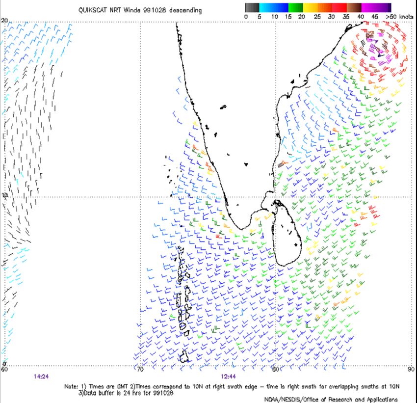
WES, User Manual

     7.6   Method 7: computing wind and pressure fields from Vmax . . . . . . . . . . . 24

8 Comparisons with observations                                                                          25
  8.1 Comparison of Radius of Maximum Wind (Rw ) and maximum wind speed                          .   .   25
  8.2 Comparison of Wind speed and direction with satellite data . . . . . . . .                 .   .   27
      8.2.1 QuickSCAT winds . . . . . . . . . . . . . . . . . . . . . . . . .                    .   .   27
      8.2.2 ERS winds . . . . . . . . . . . . . . . . . . . . . . . . . . . .                    .   .   30
      8.2.3 Comparison of WES Winds with measured ground data . . . . . .                        .   .   35

9 Comparison of different methods                                                                        37

10 Glossary of terms                                                                                     39

References                                                                                               41

A Description of used files                                                                              43
  A.1 Description of the main input file for WES  . . . . . .     .   .   .   .   .   .   .   .   43
  A.2 History points,  . . . . . . . . . . . . . . . . . . .      .   .   .   .   .   .   .   .   44
  A.3 Description of the cyclone parameters in the track file,    .   .   .   .   .   .   .   .   45
  A.4 Spiderweb file . . . . . . . . . . . . . . . . . . . . . . . . .   .   .   .   .   .   .   .   .   46
  A.5 Conversion Factors for wind speed . . . . . . . . . . . . . .      .   .   .   .   .   .   .   .   46
  A.6 Common Errors and Suggested Solutions in WES . . . . . .           .   .   .   .   .   .   .   .   48

iv                                                                                           Deltares
List of Figures

List of Figures
   2.1     Tropical cyclone winds on a circular grid . . . . . . . . . . . . . . . . . . . .                4
   2.2     Definition of the spiderweb grid . . . . . . . . . . . . . . . . . . . . . . . .                 4

   3.1     Screen shot from WES requesting the name of the main input file      .   .   .   .   .   .   .   7
   3.2     Specifying the name of the main input file . . . . . . . . . . . .   .   .   .   .   .   .   .   7
   3.3     Screen shot from WES while processing . . . . . . . . . . . .        .   .   .   .   .   .   .   8
   3.4     Screen shot from WES showing error in running WES . . . . . .        .   .   .   .   .   .   .   8

   5.1     Example of calculated wind speed for given A and B values . . . . . . . . . . 11
   5.2                                                                       a|| > ||⃗b|| . 13
           Asymmetric wind due to translation of the cyclone. Wind vectors ||⃗

   6.1     A and B value computed using two different methods . . . . . . . . . . . . 16
   6.2     Left: Central pressure drop depicted agains maximum wind for 13 hurricanes
           in USA between 2000 – and 2005 data;
           Right: Comparison between the empirical relation to hurricane Ike data (data
           source: http://weather.unisys.com/hurricane). . . . . . . . . . . . . . . . . 17
   6.3     Central pressure vs maximum wind for WES, HURDAT observations and Hol-
           lands’ P–W model and Dvorak for the dependent dataset (source: Holland
           (2008)) . . . . . . . . . . . . . . . . . . . . . . . . . . . . . . . . . . . . 18
   6.4     B as a function of Maximum wind speed (Vmax ) for Indian tropical cyclones . 18
   7.1     A and B value computed using two different methods . . . . . . . . . . . . 22
   7.2     Left: Central pressure drop depicted agains maximum wind for 13 hurricanes
           in USA between 2000 – and 2005 data; Right: Comparison between the empir-
           ical relation to hurricane Ike data (data source: http://weather.unisys.com/hurricane).
            . . . . . . . . . . . . . . . . . . . . . . . . . . . . . . . . . . . . . . . . 23
   7.3     Central pressure vs maximum wind for WES, HURDAT observations and Hol-
           lands’ P–W model and Dvorak for the dependent dataset (source: Holland
           (2008)) . . . . . . . . . . . . . . . . . . . . . . . . . . . . . . . . . . . . 24
   7.4     B as a function of Maximum wind speed (Vmax ) for Indian tropical cyclones . 24
   8.1     (from top to bottom) Comparison between the observed and computed Radius
           of Maximum Wind and maximum wind speed for Vizag, Kakinada, and Orissa
           Cyclones . . . . . . . . . . . . . . . . . . . . . . . . . . . . . . . . . . . 26
   8.2     QuickSCAT wind measured at 28/10/1999 (Orissa Cyclone - 05B). Black coloured
           wind barbs indicates rain contaminated data. . . . . . . . . . . . . . . . . . 27
   8.3     Comparison of WES winds and direction with derived winds from QuickSCAT
           satellite for 4 different sectors (Orissa Cyclone) . . . . . . . . . . . . . . . . 28
   8.4     Comparison of WES winds and direction with derived winds from QuickSCAT
           satellite for 4 different sectors (Cuddalore Cyclone) . . . . . . . . . . . . . . 29
   8.5     Comparison of ERS and parametric wind speeds and directions (Method A)
           on three radial cross sections on 28/10/1999 at 0400 Z. Triangles represent
           ERS data, crosses model data . . . . . . . . . . . . . . . . . . . . . . . . 31
   8.6     Comparison of ERS and parametric wind speeds and directions (Method B) on
           four radial cross sections on 28/10/1999 at 0400 Z. Triangles represent ERS
           data, crosses model data . . . . . . . . . . . . . . . . . . . . . . . . . . . 32
   8.7     Comparison of ERS and parametric wind speeds and directions (Method A) on
           four radial cross sections on 28/11/2000 at 0400 Z. Triangles represent ERS
           data, crosses model data . . . . . . . . . . . . . . . . . . . . . . . . . . . 34
   8.8     Comparison of ERS and parametric wind speeds and directions (Method B) on
           four radial cross sections on 28/11/2000 at 0400 Z. Triangles represent ERS
           data, crosses model data . . . . . . . . . . . . . . . . . . . . . . . . . . . 35

Deltares                                                                                                    v
WES, User Manual

     8.9   Comparison of WES generated wind speed and direction with ground obser-
           vation . . . . . . . . . . . . . . . . . . . . . . . . . . . . . . . . . . . . . 36

     9.1   Computed Katrina wind speed on the 25th of August 2005 for 6 different meth-
           ods in WES . . . . . . . . . . . . . . . . . . . . . . . . . . . . . . . . . . 38

     A.1   Gust factors for cyclone wind speed (Curve C) as a function of time (Krayer
           and Marshall, 1992). . . . . . . . . . . . . . . . . . . . . . . . . . . . . . 47

vi                                                                                  Deltares
List of Tables

List of Tables
   5.1     Wind conversion factor from 1 minute (60 sec) average to 10 minutes (600
           sec) average from Harper et al. (2010). . . . . . . . . . . . . . . . . . . . . 13

Deltares                                                                                   vii
WES, User Manual viii Deltares
1 A Guide to the manual
      This user manual provides detailed information on running of WES program, version 3.3. To
      make this manual more accessible we will briefly describe the contents of each chapter and
      appendices.

      Chapter 2: Introduction, provides an overview of the WES functions, area of applications
      and the software and hardware configurations of WES.

      Chapter 3: Getting Started, gives a brief overview of the input files required, data flow within
      the program, the output files of the program and finally, the steps executed by WES.

      Chapter 4: Files description, provides practical information of the model input files

      Chapter 5: Conceptual description, describes the equations in WES.

      Chapter 7: The approach in WES, describes a number of methods available in WES to
      generate the the wind and pressure fields.

      Chapter 8: Comparisons with observations, comparison of numerical results and obser-
      vations of 4 different tropical cyclones.

      Chapter 9: Comparison of different methods, comparison of wind and pressure fields
      generated with different methods in WES.

      Chapter 10: Glossary of terms, contains a list of terms and abbreviations used in this man-
      ual and their explanations.

      References, provides a list of publications referenced by this manual.

      Appendix A: Description of used files, gives a description of all the files that can be used
      in WES. This information is required for generating some files manually or by other means of
      other utility programs.

1.1   Changes with respect to previous versions

       Version      Description

       3.32.01      Output on history points can now be generated.

       3.32.00      Default of radius of maximum wind Rmax is changed from 13.5 [nmi] to
                    25[nmi].
                    Input file format of the -file is changed.

       3.31.00      In 2014, the method of computation has been changed. In previous versions
                    (3.30.01 and earlier), the translation speed is added to the computed winds
                    which produced maximum wind speed that is higher than the maximum mean
                    speed specified. In the latest version this translation speed is taken into ac-
                    count prior to the computation. Therefore, when repeating the test cases de-
                    scribed the resulting wind speed will be slightly lower than mentioned in this
                    report.

      Deltares                                                                                1 of 50
WES, User Manual 2 of 50 Deltares
2 Introduction
Accurate depiction of the inundation requires the accurate computation of the Storm Surge
that again depends on the accuracy of the wind forcing it receives.
Tropical cyclone winds usually are accounted for in the Numerical Weather Prediction (NWP)
data. However, the grid resolution used in these models is usually not sufficient to accurately
represent the strong variations on the wind gradients near its centre due to low grid resolution.
Furthermore, the deficiencies in the parameterisation of Cumulus Convection in NWP models
do not bring out the tropical cyclone features in their true intensity and size. Hence, the
wind and pressure in the tropical cyclone that are predicted by these models are generally
underestimated. To overcome this difficulty, all meteorological agencies resort to supply some
bogus data to bring out the tropical cyclone in the analysis. The methods used to generate
winds are by Rankine Vortex or by generating some synthetic vortex or by the technique
suggested by Holland (1980). The winds generated with this approach are geostrophic in
nature. Asymmetry, which is usually encountered in the observed wind field, is brought out
by vectorial addition of the translatory movement of the tropical cyclone. For the detailed
description of this scheme we refer to chapter 8 of this document.
For storm surge simulations with Delft3D-FLOW, a Wind Enhance Scheme (WES) following
Holland (1980) has been devised to generate tropical cyclone wind field. The program com-
putes surface winds and pressure around the specified location of a tropical cyclone centre
and given a number of tropical cyclone parameters (track data: i.e. maximum wind speed,
pressure drop, radius of maximum wind and positions of the tropical cyclone). The tropical cy-
clone track data given by any Meteorological Agency can be taken by WES. However, JTWC,
is the only agency that predicts sustained maximum winds at regular intervals.
The scheme was initially developed by the UK Met Office. Further improvements to the
method have been applied to make the program more robust and yield more reliable and
consistent results. The program also calculates the radius of the maximum winds offering a
possibility to compare the output with Radius of Maximum Winds (Rmw ) derived from radar
and satellite observations.
The output of WES is suitable as input for Delft3D-FLOW and D-Flow FM, to simulate a storm
surge.
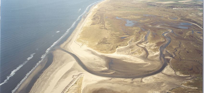
2.1 Functions and data flow of WES
The main functions and data flow of WES is to synthesize the tropical cyclone wind and
pressure drop on a circular or ‘spiderweb’ type grid (see Figure 2.1).
Deltares 3 of 50WES, User Manual
Figure 2.1: Tropical cyclone winds on a circular grid
2.2 Definition of the circular or the ‘spiderweb’ grid
For the synthesising of the tropical cyclone wind, an elegant technique has been adopted
requiring data on a polar co-ordinate grid centred on the centre of the tropical cyclone (Stelling,
1999). On this, so-called ’spiderweb’ grid, the tropical cyclone wind and pressure fields are
generated. The number of grid points in the spiderweb both in the radial and in the tangential
direction is user specifiable. The radius of the tropical cyclone must be specified by the user.
If the radius is changed, the grid cell size will vary according to number of grid cells specified.
Figure 2.2: Definition of the spiderweb grid
4 of 50 DeltaresIntroduction
2.3 Overview of the in- and output files
Input files
The following input files are needed to run WES:
file: This is the main input file for WES. The files contain information re-
garding input and output files and WES run options.
file: This file contains the tropical cyclone track information that is either
created manually (by editing it) or by another separate program.
The ‘∗’ sign above represents arbitrary filename. It is advisable however to use a filename
containing date and time stamp for all the files.
Output files
WES produces the following output files:
file: A file containing the synthesised tropical cyclone wind speed and
pressure (drop) on a polar co-ordinate grid or the spiderweb grid
(see detailed description in section A.6).
file: A diagnostic or the log file containing the steps carried out by WES +
some intermediary results. It may also contain ERROR and WARN-
ING messages from the program in case they occurred, so appropri-
ate actions may be taken to correct them.
The name above represents the basename that is identical to the input filename contained in
the file.
Deltares 5 of 50WES, User Manual 6 of 50 Deltares
3 Getting Started

3.1   How to run WES
      When invoking wes on the commandline, one may specify the input file  manually as
      the program argument. If not specified, it will ask you to specify this file name, see Figure 3.1.

                 Figure 3.1: Screen shot from WES requesting the name of the main input file

      Type the  file name as indicated in Figure 3.2.

                             Figure 3.2: Specifying the name of the main input file

      Once the input file is given, the details of the input files are read and processed.

      The screen shots of WES when running is given, Figure 3.3.

      Deltares                                                                                  7 of 50
WES, User Manual
Figure 3.3: Screen shot from WES while processing
The detailed information regarding the processed input can also be seen in one of the output
files of WES .
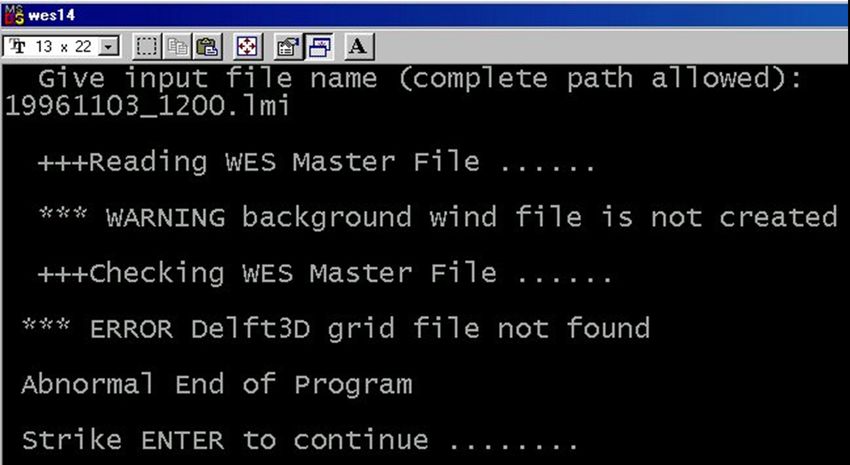
If there are any errors in the input file WES will stop and it will generate the message “Abnor-
mal end of the program” (see Figure 3.4).
Figure 3.4: Screen shot from WES showing error in running WES
If no error is encountered, WES will produce the output files: file and .
8 of 50 Deltares4 Files description
4.1 The main Input file file
The main input file must be available describing the options for running WES (e.g. the details
about the spiderweb grid size, the required extent of the diagnostic file - brief or detailed, etc.).
For a detailed description of all the parameters in the file, see section A.1.
4.2 History points, file
History points are defined by their location. The locations need to be specified by their
spherical coordinates (longitude, latidude: λ, ϕ) and their name in a file, preferred exten-
sion . For these points time series are written to the diagonostic file for windspeed
[knots] and nautical direction [degrees].
Example:
269.632 30.050 'EastBank1'
270.043 29.263 'GrandIsle'
270.593 28.932 'PilotsStEast'
270.56 30.282 'Waveland'
269.582 29.777 'WestBank1'
For a detailed description of file file, see section A.2.
4.3 Creating a track file
This file may be edited manually. This file contains the main information on the tropical cyclone
parameters:
⋄ the initial and predicted positions of the storm centre (in geographical co-ordinates),
⋄ the direction and speed of movement of the storm centre during the previous 6 hours,
⋄ the intensity of the storm in terms of associated maximum winds and the corresponding
pressure drop in Pascal.
For a detailed description of all the parameters in the file, see section A.3
4.4 Possible input parameters with respect to the tropical cyclone intensity
The important input parameters for WES that determines the tropical cyclone wind intensity
are:
A This parameter along with the parameter B below, determines the radius at
which maximum wind speeds occur. It is very unlikely that the value of this
parameter is known.
B This parameter determines the shape of the wind and pressure profile as a
function of distance from the storm centre. In some regions B has been de-
termined from climatological data and you may wish to use this value. In the
modified form, the B is calculated from Vmax , which can vary from day to day
in a given tropical cyclone. Hence B value not kept constant between the initial
and predicted intensities of tropical cyclone.
Vmax The maximum sustained wind in the tropical cyclone [knots]. This parameter is
compulsory. It is estimated from satellite data and other observed data.
Deltares 9 of 50WES, User Manual
Rmax The radius of maximum sustained wind in the tropical cyclone ([nmi]) associated
with the parameter Vmax mentioned earlier. When not specified then a default
value of 25 [nmi] will be assumed.
pdrop Represents the difference between the ambient and central pressures [hPa].
This parameter is estimated from satellite images, or may be computed using
√
the following relation Vmax = C pdrop (see chapter 8). In some cases pdrop
and Vmax will be the only pieces of data available.
Radius of 35, 50 & 100 knots wind
These parameters are estimated from observations and are reported in JTWC
bulletins.
These parameters are to be specified in a certain combination in order to allow WES to pro-
duce the desired output (see chapter 7).
The values for the parameters described above may be obtained from tropical cyclone ad-
visories produced by JTWC, UKMO, IMD, JMA or any other Meteorological institutes in the
world. In all advisories, the present and forecast positions of the tropical cyclones are given.
The tropical cyclone intensity parameter however is only specified in the JTWC (Hawaii) ad-
visory in the form of prevailing and forecast maximum winds or in the IMD tropical cyclone
bulletins as prevailing tropical cyclone intensity (specified in categories). Specifying the posi-
tions, the prevailing and the expected wind speeds and pressure drops information are suf-
ficient to synthesise the tropical cyclone winds. In this case certain assumptions have to be
made about the model parameters (see chapter 8).
JTWC advisory also contains information on the present and expected radius of 100 knots
wind (R100 ), 50 knots wind (R50 ), and 35 knots wind (R35 ) as a function of position (c.q.
time). In this case the assumptions mentioned earlier are not required and WES can use the
above radii in order to find an optimal fitting of the synthesised winds to the observed values.
When not available or not used the related columns for these parameters in the -file
must be filled with the “Missing Index” value (= 1.0 × 1030 ).
A detailed description of the file is given in Appendix A.3. Also of importance is the
explanation on how WES will treat the different options and when redundant information is
specified in this file.
4.5 The diagnostic file
The diagnostic file (): In the file, the option EXTENDED_REPORT enables
the user to specify whether an extended diagnostics are to be produced or not. Extended
diagnostics include process-logging, extensive error and warning messages, etc. Compact
diagnostic will only contain process-logging and main error messages. If the user mentions
“YES” for EXTENDED_REPORT, extended diagnostics will be produced else compact diag-
nostics will be produced.
In the extended mode the following information are dumped to the diagnostic file.
1 The contents of the input file, -file.
2 The contents of tropical cyclone track file, , read including the computed constants
and parameters such as A, B and pdrop , the pressure drop for different time step.
3 Summary of data in the spiderweb file for Delft3D, which consists of date and time of the
tropical cyclone position, maximum wind speed in [knots], its direction and radius of the
maximum winds and direction in which it occurs.
10 of 50 Deltares5 Conceptual description
Cyclone wind fields are generated around the given centre positions of the storm, following
Holland’s method in order to obtain the wind and pressure fields (above sea surface) on a
high-resolution grid. The parametric model that has been adopted in WES is based upon
Holland (1980). And it has been improved slightly by introducing asymmetry. This asymmetry
is brought about by applying the translation speed of the cyclone centre displacement as
steering current and by introducing rotation of wind speed due to friction.
This model has basically five parameters:
1 the location of the cyclone centre,
2 the radius of maximum wind,
3 the maximum wind speed,
4 the central pressure and
5 the current motion vector of the vortex.
5.1 Brief description of Holland’s model
Following Holland, the geostrophic wind speed Vg of a cyclone is expressed as:
rf
q
Vg (r) = ABpdrop exp(−A/rB )/ρrB + r2 f 2 /4 − (5.1)
2
where
r distance from the centre of the cyclone,
f Coriolis parameter,
ρ density of air (assumed to be constant equal to 1.10 kg m−3 ),
pdrop = pn − pc
pn ambient pressure (theoretically at infinite radius, however in this model the
average pressure over the model domain is used)
pc central pressure,
A, B parameters.
Wind speed as functions of A & B
100.00
B= 1.75 A= 5.00E+06
B= 1.5 A= 5.00E+06
B= 1.25 A= 5.00E+06
B= 1.25 A= 1.00E+06
75.00 B= 1.25 A= 5.00E+05
W in d s p e e d (m /s )
50.00
25.00
0.00
0 50000 100000 150000 200000 250000 300000
Distance (m)
Figure 5.1: Example of calculated wind speed for given A and B values
Parameters A and B are determined empirically. Physically parameter A determines the
relation of the pressure or wind profile relative to the origin, and parameter B defines the
shape of the profile, see Figure 5.1. Holland states that for plausible ranges of central and
Deltares 11 of 50WES, User Manual
ambient pressures and radii of maximum wind speeds B is constrained to be between 1 and
2.5.
In the region of maximum winds the Coriolis force is small in comparison to the pressure gradi-
ent and centrifugal forces, and therefore the air is in cyclostrophic balance. The cyclostrophic
wind Vc at a distance r in this region is given by:
q
Vc (r) = AB(pdrop ) exp(−A/rB )/ρrB (5.2)
By setting d Vc /dr = 0, the radius of maximum winds (Rw ) can be obtained and is given as
follows:
Rw = A1/B (5.3)
The Rw is independent of the relative values of ambient and central pressure and it is defined
entirely by the scaling parameters A and B . Substituting Equation (5.3) back into Equa-
tion (5.2) yields an expression for the maximum wind speed as follows:
q
Vmax = Bpdrop /ρ e (5.4)
where e is the base of the natural logarithm (=2.71828. . . ).
Parameters A and B can now be expressed as functions of measurable quantities as follows:
B
A = Rw (5.5)
2
ρ e Vmax
B= (5.6)
pdrop
and the central pressure drop is given by
2
ρ e Vmax
pdrop = (5.7)
B
By substituting equations 5.5 and 5.6 into equation 5.1 we can also express the geostrophic
wind Vg as function of Rw :
p rf
Vg (r) = (Rw /r)B Vmax
2 exp(1 − (Rw /r)B ) + r2 f 2 /4 − (5.8)
2
The equations above are valid for geostrophic winds. Before deriving A and B the wind speed
and pressure values are now scaled to their geostrophic values.
5.2 Further improvements to the original model
After determining the values of parameter A and B , the cyclone winds as a function of dis-
tance r and direction θ on a spiderweb like grid can be computed. The computed winds are
then adjusted to account for the asymmetry introduced by the interaction of the cyclone with
the steering flow (Chan and Gray, 1982) by adding the translatory movement of the cyclone
to the existing wind field. On the northern hemisphere this vectorial addition increases the
winds on the right hand side of the direction of the cyclone movement and reduces the winds
on the left hand side and the other way around on the southern hemisphere, see Figure 5.2,
so bringing out an asymmetry in the wind field.
12 of 50 DeltaresConceptual description
Cyclone track Cyclone track
a
a
b
b
Northern hemisphere Southern hemisphere
Figure 5.2: Asymmetric wind due to translation of the cyclone. Wind vectors ||⃗a|| > ||⃗b||
The wind direction (northern hemisphere) is rotated 20◦ in the anti clock-wise (cyclonic) di-
rection so that the wind spirals in towards the centre (Shea and Gray, 1973) to account for
the frictional effects. Also for the same reason a reduction factor of 0.7 is applied for the
geostrophic wind to generate winds at 10 meters above mean sea level. For wind speed this
involves a multiplication by a factor represented by Preduce , and for pressure drop divided by
2
Preduce . Preduce is currently set to 0.7, the appropriate value over water1 .
5.3 Conversion factors
Any wind speed that is mentioned in the advisories and or computed by the NWP models is
defined as wind speed that has been averaged over a certain period of time. For example,
JTWC advisory mentions wind speeds that are based on 1-minute average while the IMD
uses the wind speed based on 3-minutes average. For storm surge simulations, at least 10
minute average winds should be applied.
To allow a specification of maximum wind speed, Vmax , originating from any sources and in
order to enable WES to compute wind speed in consistent manner for your use, a conversion
factor is introduced. It is used to convert maximum wind speed specified (y -minute averaged,
input) in the (input) track file to the required, x-minute, averaged (output) wind data required
by the user.
Conversion factor from 1 minute average to 10 minutes average for different areas can be
obtained by Harper et al. (2010) which for convenience has been copied below:
Table 5.1: Wind conversion factor from 1 minute (60 sec) average to 10 minutes (600 sec)
average from Harper et al. (2010).
Vmax600 = K Vmax60 At-Sea Off-Sea Off-land In-land
K 0.93 0.90 0.87 0.84
As in Delft3D no distinction is made between land and sea, a value between 0.9 and 0.93 is
recommended.
Another way to determine the conversion value is by determining the inverse ratio of the Gust
factor for those averaging periods respectively. For a detailed overview and treatment of the
Gust factor and the conversion factor we refer to section A.4.
1
WES does not account for frictional effects of land
Deltares 13 of 50WES, User Manual 14 of 50 Deltares
6 The approach in WES
      Equation (5.8) synthesises cyclonic winds assuming that the values of parameters A and B
      are known. However, in practical situation these parameters are usually not directly available.
      Consequently, in operational / forecast mode the tropical cyclone winds and pressure field is
      computed based on (measured/observed/forecast) physical quantities that are reported in the
      tropical cyclone advisories: Vmax , Rw , Pressure drop and or Radius of 100, 65, 50 and 35
      knots wind (if and when the wind exceeds the associated speed).

      Unfortunately cyclone advisories originating from different meteorological agencies do not
      contain identical information for which a standard procedure can be developed. Below we
      summarise the contents of some of the advisories:

      ⋄ Cyclone advisories from UK Met Office contain the present and 72 hours forecast of the
        cyclone positions accompanied by a qualitative description of the changes in the cyclone
        strength (intensifying, weakening etc.).
      ⋄ JTWC advisories contains the present and 48 hours forecast of the cyclone positions
        accompanied by a quantitative description of the cyclone strength with the help of four
        parameters:
          1   Maximum sustainable winds (Vmax ) at present positions,
          2   Radius of 35 knots wind (R35 ) at present and future positions,
          3   Radius of 50 knots wind (R50 ) at present and future positions and
          4   Radius of 100 knots wind (R100 ) at present and future positions.
      ⋄ IMD advisories contain the present and 36 hours forecast positions of the tropical cyclone
         and a qualitative description of the changes in its strength (intensifying, weakening etc.)
      ⋄ In all advisories the present tropical cyclone translation speed and its direction are men-
         tioned.

      The method to compute the wind and pressure fields in WES depends on the tropical cyclone
      parameters specified and is described below.

6.1   Method 1: computing wind and pressure fields from Vmax , A and B
      In case the parameters A, B and Vmax are specified, then the wind and pressure fields can
      directly be computed using equations Equation (5.7) and Equation (5.8).

6.2   Method 2: computing wind and pressure fields from Vmax , R35 , R50 and R100
      The available data (wind speed associated with R35 , R50 and R100 ), together with Vmax , can
      been used to fit Equation (5.1) with these parameters and obtain the appropriate values of A
      and B . The value of Rw is then determined from Equation (5.3).

      The method described here has been tested on a number of tropical cyclones in India and
      Vietnam. As an example Figure 7.1 shows the results in one of the case tested namely the
      Orissa Cyclone (05B) – 1999. The method is found to produce consistent result when at least
      3 out of 4 values of R35 , R50 and R100 are available (i.e. in case of a strong tropical cyclone).
      Otherwise the method is less dependable.

      Deltares                                                                                 15 of 50
WES, User Manual
Figure 6.1: A and B value computed using two different methods
6.3 Method 3: computing wind and pressure fields from Vmax , pdrop and Rw
If all the three parameters Vmax , pdrop and Rw are known then the tropical cyclone wind field
can be easily computed using Equations 5.5, 5.6 and 5.8.
However, usually these parameters are not available all at the same time. So the following
solutions are available in WES (see next sections).
6.4 Method 4: computing wind and pressure fields from Vmax , pdrop (Rw is not known)
If the value of Rw is not known or specified then a default value of 25 km for Rw will be
assumed.
6.5 Methods 5 and 6: Computing wind and pressure fields from Vmax and Rw (pdrop is not
known)
When the pressure drop is not specified two methods can be applied:
1 pdrop based on empirical model based on US hurricane statistics.
2 pdrop based on empirical model for Indian tropical cyclones.
6.5.1 Method 5: Computing wind and pressure fields from Vmax and Rw (pdrop is not
known), pdrop based on empirical model based on US hurricane statistics
Based on data of 13 hurricanes (Ida, Bill, Hannah, Gustav, Dolly, Dean, Dennis, Emily, Katrina,
Rita, Wilma, Charley and Ivan1 ); that occurred in USA between the year 2000 and 2005, we
have derived an empirical relation between the pressure drop and quadrate of maximum wind
speed (as suggested by Equation (5.7)). This empirical relation reads (See Figure 7.2 left):
2
pdrop = 2Vmax (6.1)
Substituting this to Equation (5.7) yields a B value equal to:
1
B = ρ e = 1.563. (6.2)
2
1
source: http://weather.unisys.com/hurricane
16 of 50 DeltaresThe approach in WES
Wind speed and Pdrop relation Wind speed and Pdrop relation y = 2x 2
20000
EMPIRICAL RELATION 10000
WES derived relation
ALL (excl. IKE)
IKE
Power (EMPIRICAL RELATION)
15000 y = 2x 2 Power (WES derived relation)
P re s s u re d ro p (P a )
P r e s s u r e d r o p (P a )
10000 6000
5000
2000
0
30 50 70
0 20 40 60 80 100
Wind Speed (m/s) Wind speed (m/s)
Figure 6.2: Left: Central pressure drop depicted agains maximum wind for 13 hurricanes
in USA between 2000 – and 2005 data;
Right: Comparison between the empirical relation to hurricane Ike data (data
source: http://weather.unisys.com/hurricane).
This relation is applied to data from Hurricane Ike (see Figure 7.2 right) seems to system-
atically underestimate the pressure drop for winds < 50 m/s and slightly overestimate the
pressure (drop) for wind speed > 50 m/s. Lower wind speed in this graph depicts the winds
after the 8th of September. The systematic bias during this period may be caused by the fact
that the ambient pressure during the last stages of Ike is slightly lower than 1010 mbar.
Once the value of B is determined, subsequently, the value of pdrop can be determined.
Holland (2008) devised a new empirical relation for relating maximum winds to central pres-
sure in tropical cyclones. He determined a derivative of the Holland B parameter, Bs , which
relates the pressure drop directly to surface winds. This parameter Bs is a function of pres-
sure drop at the centre of the tropical cyclone, intensification rate, latitude, and translation
speed.
To compare the empirical relation given by Equation (7.1) to the recent Hollands findings,
Figure 7.3 is presented.
Deltares 17 of 50WES, User Manual
Figure 6.3: Central pressure vs maximum wind for WES, HURDAT observations and Hol-
lands’ P–W model and Dvorak for the dependent dataset (source: Holland
(2008))
6.5.2 Method 6: Computing wind and pressure fields from Vmax and Rw (pdrop is not
known), pdrop based on empirical model for Indian tropical cyclones
The following empirical method has been devised after investigating a number of tropical
cyclones in the Bay of Bengal as an option after the observation that method 2 often fails to
produce a reliable result, due to limited number of parameters.
The method is based on practice applied by IMD that uses a constant value to relate the
maximum sustained wind speed with the pressure drop. The value of B is subsequently de-
termined by fitting the data from a number of tropical cyclone occurring in India. This relation
is described by a linear function where B is set equal to 1.18 for 20 knot winds (approximately
10 m/s). It linearly increases towards a value of 1.55 for wind speed equals 150 knots (ap-
proximately 77 m/s; see Figure 7.4). Once the value of B is determined, subsequently, the
value of pdrop can be determined.
B = Vm2 ?e / pd 1.352308
2.50
B derived directly form hindcast data
B as a function of wind speed used in W ES
2.25
2.00
1.75
B
1.50
1.25
1.00
0 10 20 30 40 50 60 70 80
W ind speed (m /s)
Figure 6.4: B as a function of Maximum wind speed (Vmax ) for Indian tropical cyclones
18 of 50 DeltaresThe approach in WES
For A, a value between 4.1 · 106 and 4.2 · 106 has been applied. An example of the result is
shown in Figure 7.1 for the Orissa Cyclone (05B) – 1999 test case.
6.6 Method 7: computing wind and pressure fields from Vmax
The only data used in this method is the maximum wind speed Vmax . Through some error
minimisation procedure the value of A and Rw is determined. However this method is proven
not to be robust and is only maintained in WES for backward compatibility reason. The use of
this method is no longer recommended.
Deltares 19 of 50WES, User Manual 20 of 50 Deltares
7 The approach in WES
      Equation (5.8) synthesises cyclonic winds assuming that the values of parameters A and B
      are known. However, in practical situation these parameters are usually not directly available.
      Consequently, in operational/forecast mode the tropical cyclone winds and pressure field is
      computed based on (measured/observed/forecast) physical quantities that are reported in the
      tropical cyclone advisories: Vmax , RW , Pressure drop and or Radius of 100, 65, 50 and 35
      knots wind (if and when the wind exceeds the associated speed).

      Unfortunately cyclone advisories originating from different meteorological agencies do not
      contain identical information for which a standard procedure can be developed. Below we
      summarise the contents of some of the advisories:

      ⋄ Cyclone advisories from UK Met Office contain the present and 72 hours forecast of the
        cyclone positions accompanied by a qualitative description of the changes in the cyclone
        strength (intensifying, weakening etc.).
      ⋄ JTWC advisories contains the present and 48 hours forecast of the cyclone positions
        accompanied by a quantitative description of the cyclone strength with the help of four
        parameters:
          1   Maximum sustainable winds (Vmax ) at present positions,
          2   Radius of 35 knots wind (R35 ) at present and future positions,
          3   Radius of 50 knots wind (R50 ) at present and future positions and
          4   Radius of 100 knots wind (R100 ) at present and future positions.
      ⋄ IMD advisories contain the present and 36 hours forecast positions of the tropical cyclone
         and a qualitative description of the changes in its strength (intensifying, weakening etc.)
      ⋄ In all advisories the present tropical cyclone translation speed and its direction are men-
         tioned.

      The method to compute the wind and pressure fields in WES depends on the tropical cyclone
      parameters specified and is described below.

7.1   Method 1: computing wind and pressure fields from Vmax , A and B
      In case the parameters A, B and Vmax are specified, then the wind and pressure fields can
      directly be computed using equations Equation (5.7) and Equation (5.8).

7.2   Method 2: computing wind and pressure fields from Vmax , R35 , R50 and R100
      The available data (wind speed associated with R35 , R50 and R100 ), together with Vmax , can
      been used to fit Equation (5.1) with these parameters and obtain the appropriate values of A
      and B . The value of Rw is then determined from Equation (5.3).

      The method described here has been tested on a number of tropical cyclones in India and
      Vietnam. As an example Figure 7.1 shows the results in one of the case tested namely the
      Orissa Cyclone (05B) – 1999. The method is found to produce consistent result when at least
      3 out of 4 values of R35 , R50 and R100 are available (i.e. in case of a strong tropical cyclone).
      Otherwise the method is less dependable.

      Deltares                                                                                 21 of 50
WES, User Manual
Figure 7.1: A and B value computed using two different methods
7.3 Method 3: computing wind and pressure fields from Vmax , Pdrop and Rw
If all the three parameters Vmax , Pdrop and Rw are known then the tropical cyclone wind field
can be easily computed using Equations 5.5, 5.6 and 5.8.
However, usually these parameters are not available all at the same time. So the following
solutions are available in WES (see next sections).
7.4 Method 4: computing wind and pressure fields from Vmax , Pdrop (Rw is not known)
If the value of Rw is not known or specified then a default value of 25 km for Rw will be
assumed.
7.5 Methods 5 and 6: Computing wind and pressure fields from Vmax and Rw (Pdrop is not
known)
When pressure drop is not specified two methods can be applied:
7.5.1 Method 5: Pdrop based on empirical model based on US hurricane statistics
Based on data of 13 hurricanes (Ida, Bill, Hannah, Gustav, Dolly, Dean, Dennis, Emily, Katrina,
Rita, Wilma, Charley and Ivan1 ); that occurred in USA between the year 2000 and 2005, we
have derived an empirical relation between the pressure drop and quadrate of maximum wind
speed (as suggested by Equation (5.7)). This empirical relation reads (See Figure 7.2 left):
2
Pdrop = 2Vmax (7.1)
1
source: http://weather.unisys.com/hurricane
22 of 50 DeltaresThe approach in WES
Substituting this to Equation (5.7) yields a B value equal to:
1
B = ρ e = 1.563. (7.2)
2
Wind speed and Pdrop relation Wind speed and Pdrop relation y = 2x 2
20000
EMPIRICAL RELATION 10000
WES derived relation
ALL (excl. IKE)
IKE
Power (EMPIRICAL RELATION)
15000 y = 2x 2 Power (WES derived relation)
P re s s u re d ro p (P a )
P r e s s u r e d r o p (P a )
10000 6000
5000
2000
0
30 50 70
0 20 40 60 80 100
Wind Speed (m/s) Wind speed (m/s)
Figure 7.2: Left: Central pressure drop depicted agains maximum wind for 13 hur-
ricanes in USA between 2000 – and 2005 data; Right: Compari-
son between the empirical relation to hurricane Ike data (data source:
http://weather.unisys.com/hurricane).
This relation is applied to data from Hurricane Ike (see Figure 7.2 right) seems to system-
atically underestimate the pressure drop for winds < 50 m/s and slightly overestimate the
pressure (drop) for wind speed > 50 m/s. Lower wind speed in this graph depicts the winds
after the 8th of September. The systematic bias during this period may be caused by the fact
that the ambient pressure during the last stages of Ike is slightly lower than 1010 mbar.
Once the value of B is determined, subsequently, the value of Pdrop can be determined.
Holland (2008) devised a new empirical relation for relating maximum winds to central pres-
sure in tropical cyclones. He determined a derivative of the Holland B parameter, Bs , which
relates the pressure drop directly to surface winds. This parameter Bs is a function of pres-
sure drop at the centre of the tropical cyclone, intensification rate, latitude, and translation
speed.
To compare the empirical relation given by Equation (7.1) to the recent Hollands findings,
Figure 7.3 is presented.
7.5.2 Method 6: Pdrop based on empirical model for Indian tropical cyclones
The following empirical method has been devised after investigating a number of tropical
cyclones in the Bay of Bengal as an option after the observation that method 2 often fails to
produce a reliable result, due to limited number of parameters.
The method is based on practice applied by IMD that uses a constant value to relate the
maximum sustained wind speed with the pressure drop. The value of B is subsequently de-
termined by fitting the data from a number of tropical cyclone occurring in India. This relation
is described by a linear function where B is set equal to 1.18 for 20 knot winds (approximately
10 m/s). It linearly increases towards a value of 1.55 for wind speed equals 150 knots (ap-
Deltares 23 of 50WES, User Manual
Figure 7.3: Central pressure vs maximum wind for WES, HURDAT observations and Hol-
lands’ P–W model and Dvorak for the dependent dataset (source: Holland
(2008))
B = Vm2 ?e / pd 1.352308
2.50
B derived directly form hindcast data
B as a function of wind speed used in W ES
2.25
2.00
1.75
B
1.50
1.25
1.00
0 10 20 30 40 50 60 70 80
W ind speed (m /s)
Figure 7.4: B as a function of Maximum wind speed (Vmax ) for Indian tropical cyclones
proximately 77 m/s; see Figure 7.4). Once the value of B is determined, subsequently, the
value of Pdrop can be determined.
For A, a value between 4.1E+06 and 4.2E+06 has been applied. An example of the result is
shown in Figure 7.1 for the Orissa Cyclone (05B) – 1999 test case.
7.6 Method 7: computing wind and pressure fields from Vmax
The only data used in this method is the maximum wind speed Vmax . Through some error
minimisation procedure the value of A and Rw is determined. However this method is proven
not to be robust and is only maintained in WES for backward compatibility reason. The use of
this method is no longer recommended.
24 of 50 Deltares8 Comparisons with observations
For comparison with observations (or derived parameters from observations) the following
tropical cyclones and parameters have been selected.
Tropical cyclone Parameter(s) compared
Name Id Year Month Radius of Wind speed Ground ob- Wind speed
Max. wind & direc- servation & direction
and Max. tion profile (wind speed (statistic –
Wind speed (QuickSCAT & direction) ERS data)
data)
Visakhapatnam (Vizag) 05B 1994 Nov ✓ - - -
Kakinada 05B 1996 Nov ✓ - - -
Orissa 05B 1999 Oct ✓ ✓ ✓ ✓
Cuddalore 03B 2000 Nov - ✓ - ✓
When comparing the computed wind with observation data, it is important to bear in mind
that the tropical cyclone centre is usually given in latitude and longitude up to a tenth of a
degree. So due to round off error the actual positions may actually differ up to ± 5 km from
the specified point. This might introduce discrepancies in the results when compared to the
observed values, especially in the region where wind gradients are high.
8.1 Comparison of Radius of Maximum Wind (Rw ) and maximum wind speed
The radius of maximum wind (Rw ) and the maximum wind speed data originates from JTWC
tropical cyclone bulletins and IMD RSMC report. Methods 2 and 6 (see chapter 7) was subse-
quently adopted to synthesise the tropical cyclone winds. The resulting wind speed was then
compared with the data.
Rw can also be compared against the radius of maximum reflectivity (Rmr ) which can be
measured by radar (Rmr is a measure of Rw ).
The JTWC provides two values for radii for 35, 50 and 100 knots winds in their bulletin. One
number represents the value for the north-eastern semicircle and the other one for remaining
areas. In the computation of the wind an average of these two values has been used. Fur-
thermore the bulletins are issued every 12 hours. To compute the wind field for every 6 hours
interpolation of these values have been applied.
Figures 8.1a to 8.1c depict the plots of radius of maximum wind and the maximum wind speed
during the life cycle of the tropical cyclone from the Vizag-1998, Kakinada-1996 and Orissa-
1999 cyclones.
Deltares 25 of 50WES, User Manual
(a) Cyclone Vizag (1998)
(b) Cyclone Kakinada (1996)
(c) Cyclone Orissa (1999)
Figure 8.1: (from top to bottom) Comparison between the observed and computed Ra-
dius of Maximum Wind and maximum wind speed for Vizag, Kakinada, and
Orissa Cyclones
In Figure 8.1c, the Orissa Cyclone case, the radius of maximum wind (Rw ) gradually de-
creased from a value of 42 km on the 26th October to a value of 7.5 km on the 29th October
when the tropical cyclone reached its peak intensity. The radius of maximum wind increases
after the tropical cyclone made landfall and became weaker. The triangles shown in the di-
agram represents the Rmr values measured by the radar at Paradip and the squares in the
diagram represents 0.5 times of the eye diameter (= radius of the eye). The reported accu-
racy of the observed data is represented in the figures by an error bar. The agreement with
Rmr and Rw in this case is remarkably good. Similar holds for the computed maximum wind
speed, especially for the winds computed using method A. Figures 8.1a and 8.1b represent
26 of 50 DeltaresComparisons with observations
the diagrams for Vizag and Kakinada cyclones. Similar conclusion can be drawn for the Vizag
cyclone case. The Rw values in the Kakinada cyclone case however, are slightly larger than
the reported Rmr value.
8.2 Comparison of Wind speed and direction with satellite data
As long as the tropical cyclone is at the ocean comparison of model result with observations
has to rely on winds derived from the satellite data, as conventional observations are hardly
available over the oceans. Fortunately, ERS satellite and more recently QuickSCAT derives
wind data from scatterometer data, despite some limitations. The accuracy of the winds is
claimed to be 1.4 m/s up to the speeds of 20 m/s and an accuracy of 10 % beyond that. The
maximum measurable speeds with the scatterometer are 50 knots (≈ 25 m/s). Hence, at
higher wind speeds comparison cannot be made. This QuickSCAT data from the year 1999
onwards is available at the site1 .
8.2.1 QuickSCAT winds
WES computed winds has been compared with QuickSCAT data for the Orissa cyclone (26-30
Oct, 1999) and Cuddalore Cyclone (27–29 Nov, 2000). The comparison is made by printing
out the graphs that have been downloaded from the above referred internet site and reading
the wind speed and direction visually.
Figure 8.2: QuickSCAT wind measured at 28/10/1999 (Orissa Cyclone - 05B). Black
coloured wind barbs indicates rain contaminated data.
Despite the fact that this method of comparison is imperfect and very error prone, it is never-
theless useful to check the main characteristics of the wind fields produced. An example plot
of QuickSCAT observed data is depicted in Figure 8.2c for the Orissa Cyclone case.
1
http://manati.wwb.noaa.gov/cgi-bin/qscat_day-1.pl
Deltares 27 of 50WES, User Manual
Figure 8.3: Comparison of WES winds and direction with derived winds from QuickSCAT
satellite for 4 different sectors (Orissa Cyclone)
The following figures depicts 4 cross-sections of the wind derived with WES. The wind speeds
and direction of the winds from QuickSCAT data are shown in each diagram at the appropriate
points. Figures 8.3 and 8.4 shows the wind speed and direction at 28th October, 1999-12UTC
(Orissa Cyclone) and 28th November, 2000-12UTC (Cuddalore Cyclone). There is a very
good agreement for wind speeds and wind directions in most of the cross-sections.
The results of WES, especially the wind speed in the Orissa case and the wind direction
in the Cuddalore case show good agreements with the satellite observations. Especially
when we bear in mind that the comparison has been done by estimating the wind speed and
direction visually from a printed graph and the fact in some occasion the wind measured was
contaminated due to rainfall.
28 of 50 DeltaresComparisons with observations
Figure 8.4: Comparison of WES winds and direction with derived winds from QuickSCAT
satellite for 4 different sectors (Cuddalore Cyclone)
Deltares 29 of 50WES, User Manual
8.2.2 ERS winds
Comparison with ERS winds are carried out in a different manner as we had direct access
to the measured data (provided by the UK Met. Office). Therefore we could compare the
computed results with observation points at the exact locations. Furthermore, statistical com-
putations were possible. In the following figures and tables the comparison of the WES results,
both using method A and B, with the observed ERS derived winds are presented. When inter-
preting the figures and tables below please note that the maximum measurable speeds with
the ERS are 50 knots (≈ 25 m/s). Hence, winds at higher speeds were not included in the
analysis.
Orissa case – Method 2 (using JTWC advisories containing R35 , R50 and R100 )
A = 6.5 × 10⁶ B = 1.46 (8.1)
Vmax = 39 m/s pdrop = 31.2 hP a Rw = 46.5 km (8.2)
Number of Max distance Mean wind RMS wind Mean wind RMS wind
observa- from tropical speed er- speed er- direction direction
tion points cyclone cen- ror ror error error
tre (km) (m/s) (m/s) (degrees) (degrees)
0 100 n.a n.a n.a n.a
26 200 -3.3032 3.4498 8.4202 10.8345
108 300 -0.945 2.1533 6.9905 9.8197
245 400 0.696 2.5343 4.5498 10.2488
389 500 1.2626 2.6822 2.005 13.1879
Orissa case – Method 6 (using IMD data; Vmax and pdrop )
A = 4.04 × 10⁶ B = 1.33 (8.3)
Vmax = 41.5 m/s pdrop = 38.7 hP a Rw = 16.5 km (8.4)
Number of Max distance Mean wind RMS wind Mean wind RMS wind
observa- from tropical speed er- speed er- direction direction
tion points cyclone cen- ror ror error error
tre (km) (m/s) (m/s) (degrees) (degrees)
0 100 n.a n.a n.a n.a
26 200 -5.93 6.06 7.95 11.14
107 300 -2.99 3.73 5.58 8.79
243 400 -1.00 2.92 3.75 9.97
381 500 -0.17 2.69 1.79 13.18
30 of 50 DeltaresComparisons with observations
Figure 8.5: Comparison of ERS and parametric wind speeds and directions (Method A)
on three radial cross sections on 28/10/1999 at 0400 Z. Triangles represent
ERS data, crosses model data
Deltares 31 of 50WES, User Manual
Figure 8.6: Comparison of ERS and parametric wind speeds and directions (Method B)
on four radial cross sections on 28/10/1999 at 0400 Z. Triangles represent
ERS data, crosses model data
Cuddalore case – Method 2 (using JTWC advisories containing R35 , R50 and R100 )
A = 6.47 × 10⁶ B = 1.44 (8.5)
Vmax = 26.0 m/s pdrop = 14.0 hP a Rw = 54.5 km (8.6)
Number of Max distance Mean wind RMS wind Mean wind RMS wind
observa- from tropical speed er- speed er- direction direction
tion points cyclone cen- ror ror error error
tre (km) (m/s) (m/s) (degrees) (degrees)
28 100 -5.1043 7.7524 9.6597 34.9876
106 200 -1.6102 4.2264 11.7438 23.7
234 300 0.1976 3.2852 8.9879 18.092
409 400 1.2197 3.1091 6.2995 16.9551
627 500 1.8009 3.1167 4.9857 16.411
32 of 50 DeltaresComparisons with observations
Cuddalore case – Method 6 (using IMD data; Vmax and pdrop )
A = 4.23 × 10⁶ B = 1.37 (8.7)
Vmax = 50.4 m/s pdrop = 55.4 hP a Rw = 12.5 km (8.8)
Number of Max distance Mean wind RMS wind Mean wind RMS wind
observa- from tropical speed er- speed er- direction direction
tion points cyclone cen- ror ror error error
tre (km) (m/s) (m/s) (degrees) (degrees)
33 100 -7.60 9.08 -2.27 54.71
118 200 -2.83 4.96 5.33 34.14
253 300 -0.98 3.55 4.45 25.22
439 400 0.04 2.94 2.77 22.25
643 500 0.62 2.73 2.47 20.38
Deltares 33 of 50WES, User Manual
Figure 8.7: Comparison of ERS and parametric wind speeds and directions (Method A)
on four radial cross sections on 28/11/2000 at 0400 Z. Triangles represent
ERS data, crosses model data
34 of 50 DeltaresComparisons with observations
Figure 8.8: Comparison of ERS and parametric wind speeds and directions (Method B)
on four radial cross sections on 28/11/2000 at 0400 Z. Triangles represent
ERS data, crosses model data
Based on the figures above one might conclude that both the methods used by WES to derive
the tropical cyclone winds are comparable. However, when the maximum winds are compared
than a slightly better result is obtained by applying Method 6. The agreement between the
derived wind directions with the observed data is reasonably accurate.
The derived wind speed is quite accurate up to approximately 12 m/s. Deviations along some
cross-sections then increase up to 7 m/s on average for the wind speed values between 12
and 25 m/s. Similar to the QuickSCAT case we were not able to determine the rain contami-
nation in the measured data.
8.2.3 Comparison of WES Winds with measured ground data
Some surface wind speeds during Orissa cyclone (05B) – 1999 originating from ground ob-
servations has been collected from IMD Hyderabad Met. Office for comparison purposes. The
results are shown in Figure 8.9. From the figures it is clear that the WES winds are able to
Deltares 35 of 50WES, User Manual
reproduce the surface wind measurements with sufficient degree of accuracy. One exception
forms the results at Puri. However when a location slightly North of Puri is selected then the
results are again quite good.
Figure 8.9: Comparison of WES generated wind speed and direction with ground obser-
vation
36 of 50 Deltares9 Comparison of different methods
The different methods to compute the wind and pressure fields in WES that is made available
in WES will produce results that differs marginally from each other.
For instance, when reproducing the Katrina hurricane winds on 28th of August 2005 1200 UTC
we have applied the 7 different methods with the following parameter values:
Method Vmax Rmax R_100 R_65 R_50 R_35 B A Pd
[nmi] [nmi] [nmi] [nmi] [nmi] [Pa]
1 145 - - - - - 1.20 2E+05 -
2 145 14 28 75 118 188 - - -
3 145 14 - - - - - - 10600
4 145 - - - - - - - 10600
5 145 - - - - - - - -
6 145 - - - - - - - 10600
7 145 - - - - - - - -
The results are depicted in Figure 9.1, along with H*winds model output1 and observed data2 .
Based on the results we can conclude that for this specific case, method 7 shouldn’t be used
at all3 . For this specific case, Method 3 (or 4 where Rmax is set to a default value of 12.5
nautical miles) performs the best.
Furthermore, as expected, the asymmetry feature in WES due to interaction with land mass is
poorly represented. WES is, by design, (not yet) capable of including the effect of land mass.
1
See http://www.aoml.noaa.gov/hrd/data_sub/wind.html
2
See http://tidesandcurrents.noaa.gov/
3
As mentioned earlier only available in WES for backward compatibility reason
Deltares 37 of 50WES, User Manual
Figure 9.1: Computed Katrina wind speed on the 25th of August 2005 for 6 different meth-
ods in WES
38 of 50 DeltaresYou can also read