Velocity Gradients: Magnetic Field Tomography towards the Supernova Remnant W44 - arXiv

MNRAS 000, 1–10 (2020) Preprint 29 September 2021 Compiled using MNRAS LATEX style file v3.0

 Velocity Gradients: Magnetic Field Tomography towards the Supernova
 Remnant W44
 Mingrui Liu1 , Yue Hu1,2★ , A. Lazarian2 †
 1 Department of Physics, University of Wisconsin-Madison, Madison, WI, 53706, USA
 2 Department of Astronomy, University of Wisconsin-Madison, Madison, WI, 53706, USA
arXiv:2109.13670v1 [astro-ph.GA] 28 Sep 2021

 Accepted XXX. Received YYY; in original form ZZZ

 ABSTRACT
 As a novel approach for tracing interstellar magnetic fields, the Velocity Gradient Technique (VGT) has been proven to be effective
 for probing magnetic fields in the diffuse interstellar medium (ISM). In this work, we verify the VGT in a broader context by
 applying the technique to a molecular cloud interacting with the supernovae remnant (SNR) W44. We probe the magnetic fields
 with the VGT using CO, HCO+ , and H I emission lines and make comparison with the Planck 353 GHZ dust polarization. We
 show that the VGT gives an accurate measurement that coheres with the Planck polarization especially in intense molecular
 gas emission regions. We further study the foreground’s contribution on the polarization that results in misalignment between
 the VGT and the Planck measurements in low-intensity molecular gas areas. We advance the VGT to achieve magnetic field
 tomography by decomposing the W44 into various velocity components. We show that W44’s velocity component at ∼ 45 km
 s−1 exhibits the largest coverage and gives best agreement with Planck polarization in terms of magnetic field orientation.
 Key words: ISM:general—ISM:structure—ISM:magnetohydrodynamics—turbulence—magnetic field

 1 INTRODUCTION ∼ 11 cm and ∼ 6 cm. Nevertheless, the synchrotron polarization
 is contaminated by the effect of Faraday rotation, in particular at a
 Magnetism is of enormous significance in current astronomy stud-
 long wavelength. Therefore, there is a demand for alternative methods
 ies. Magnetized turbulence in diffuse interstellar media (ISM; Larson
 for probing magnetic fields.
 1981; Armstrong et al. 1995; Elmegreen & Scalo 2004; Mac Low &
 Klessen 2004; McKee & Ostriker 2007) are essential to critical as- The emergence of the Velocity Gradient Technique (VGT;
 trophysics problems, including star formation (see Mestel & Spitzer González-Casanova & Lazarian 2017; Yuen & Lazarian 017a; Lazar-
 1956; Schmidt 1959; Mac Low & Klessen 2004; McKee & Ostriker ian & Yuen 018a; Hu et al. 2018) provides a novel vision for inter-
 2007; Hu et al. 2020a), cosmic ray propagation as well as acceler- stellar magnetic field tracing. The technique roots in the properties
 ation (Jokipii 1966; Bell 1978; Yan & Lazarian 2002; Caprioli & of the magnetohydrodynamic (MHD) turbulence (Goldreich & Srid-
 Spitkovsky 2014). Turbulence-medicated reconnection is important har 1995), and fast turbulent reconnection (Lazarian & Vishniac
 for release of magnetic energy in astrophysical evnironments, the so- 1999). Due to the reconnection, MHD turbulent eddies are stretched
 lar flares being one of the most conspicuous examples (see Krucker along local magnetic fields that percolate the eddies and thus become
 et al. 2005; Lazarian et al. 2020 and ref. therein). The studies for Su- anisotropic (Lazarian & Vishniac 1999). The resulting anisotropy
 pernovae Remnants’ (SNRs) evolution rely crucially on magnetism induces gradients of velocity fluctuations’ amplitude to be perpen-
 and turbulence as well. dicular to the directions of local magnetic fields, which enables the
 However, probing magnetic fields in SNRs confronts technical magnetic field tracing employing the amplitude of the turbulence’s
 difficulties. Conventionally recognized techniques including starlight velocity fluctuations that are available from observations.
 polarization in interstellar dust (see Heiles 2000; Clemens et al. Multiple observational works have verified the VGT to be reli-
 012a,b, 2013) and the polarized thermal emission of aligned dust able in magnetic field tracing. The technique proved to be reliable
 (see Lazarian 2007; Andersson et al. 2015) are limited by multiple in probing magnetic fields multi-phase ISM, including diffuse neu-
 factors in deep space observations. For one, the contribution from tral hydrogen regions (Yuen & Lazarian 017a; González-Casanova
 the polarized galactic foreground obscures the local plane-of-the-sky & Lazarian 2019; Hu et al. 020a; Lu et al. 2020), nearby molecular
 (POS) magnetic fields of the SNRs. Additionally, the POS magnetic clouds (Hu et al. 019a,b, Alina et al. 2020), and the central molecular
 fields can be revealed by the polarized synchrotron emission (Planck zone (Hu et al. 021c). Previous practices have also suggested several
 Collaboration et al. 2016). It is adopted by Xiao et al. (2008, 2009) potentials of the VGT, including eliminating the foreground interfer-
 to trace the magnetic field on SNR G65.2 and S147 at wavelengths ence (Hu et al. 020a; Lu et al. 2020). The VGT is also promising
 in decomposing the magnetic field of a molecular cloud into vari-
 ous components as a function of the line-of-sight (LOS) velocity.
 ★ E-mail: yue.hu@wisc.edu Consequently, it results in a three-dimensional (3D) magnetic field
 † E-mail: alazarian@facstaff.wisc.edu tracing.

 © 2020 The Authors

2 Liu, Hu & Lazarian
 In this research, we study the VGT’s potentials as discussed above 2.3 Planck polarization
by applying the technique to the SNR W44. The W44 is a Type
 To obtain the magnetic field orientation from polarized dust emission,
II SNR locating 3 kpc away from the Sun, near = +33.◦ 750,
 we adopt the data from the 2018 publication of the Planck project
 = −1.◦ 509. The estimated age of the remnant is (0.65˘2.5) × 104
 (Planck 3rd Public Data Release 2018 of High-Frequency Instrument;
years (Sashida et al. 2013; Smith et al. 1985; Harrus et al. 1997). A
 Planck Collaboration et al. 2020) for this work. The magnetic field
massive molecular cloud closely related to W44 has been observed
 orientation is defined as = + /2, inferred from the polarization
in the region, which shows distinctive velocity components that pro-
 angle along with the polarization fraction , specifically:
vide ideal conditions for testing the VGT. We probe the magnetic
fields of the SNR molecular cloud using CO (3-2) and HCO+ (1-0) 1
 = arctan(− , )
emission lines (Sashida et al. 2013) and make a comparison with 2
 √︃ (1)
the magnetic field map inferred from the Planck 353 GHz polarized
dust emission (Planck Collaboration et al. 2020). By combing with = 2 + 2 / 
the neutral hydrogen data from the GALFA-H I survey (Peek et al. where , , and refer to the intensity of dust emission and Stokes
2018), we test the VGT’s capability in removing the foreground’s parameters, respectively. − resolves the angle conversion from the
contribution. Furthermore, we make the synergy of the VGT and the HEALPix system to the IAU system, and the multi-variables arc-
SCOUSEPY software to decompose the 3D magnetic fields of the tangent function donates the radian periodicity. We minimize the
CO (3-2) emission line. noise on the maps by smoothing the results with a Gaussian filter,
 The following contents are structured as such: in Sec. 2, we in- regularizing the nominal angular resolution of the data to 10 0 .
troduce the essential data from multiple observations that have con-
tributed significantly to this research. In Sec. 3, we present details on
the methodology for our work, including an explanation of the VGT
and the SCOUSEPY software that is critical to the study. Sec.4 is 3 METHODOLOGY
assigned to presentation of the results. We also discuss further details
 3.1 The Velocity Gradient Technique
and conclude in the final section.
 3.1.1 Theoretical consideration
 The VGT sets its basis from the advanced MHD turbulence (Gol-
 dreich & Sridhar 1995, noted as GS95 hereafter) as well as the fast
 turbulent reconnection theory (Lazarian & Vishniac 1999, noted as
2 OBSERVATIONAL DATA
 LV99 hereafter). As introduced before, the MHD turbulent eddies
2.1 CO and HCO+ emission lines exhibit anisotropy as they are elongating along the magnetic field,
 proposed by the GS95 study. The anisotropy was derived with re-
The emission lines of CO (3-2) and HCO+ (1-0) are observed with gard to the "critical balance" condition, where the cascading time
the Atacama Submillimeter Telescope Experiment (ASTE) 10m tele- ( ⊥ ) −1 is equal to the wave period ( k ) −1 , as ⊥ and k donate
scope and the Nobeyama Radio Observatory (NRO) 45m radio tele- wavevectors perpendicular and parallel to the magnetic field direction
scope, respectively (Sashida et al. 2013). respectively. Turbulent velocity ∝ 1/3 at scale accounts for the
 The HCO+ (1-0) observation sets its reference position at ( , ) = Kolmogorov-type turbulence and is the Alfvén velocity. Conse-
(+33.◦ 750, −1.◦ 509), with the FWHM beam resolution of ∼ 18 00 and quently, the quantitative expression of the MHD turbulent anisotropy
the beam efficiency of around ≈ 44%. The emission line was in Fourier space is derived as:
observed at both a wide frequency band of 512 MHz and a narrow
 2/3
frequency band of 32 MHz. For this research, we use the narrow band k ∝ ⊥ (2)
mode, which gives the velocity coverage of 1700 km/s, resulting in
 The GS95 anisotropy scaling is derived in the global reference frame,
a velocity resolution of 0.1 km/s, with a 17 00 × 17 00 × 1 km/s grid
 which is defined by the mean magnetic field. However, only the
resolution. The final map has an RMS noise level of 0.075 K (1 ) in
 anisotropy that is independent of the motion scale will be observed
the unit of brightness temperature .
 in this frame, as small eddies are blanked out by larger eddies with the
 The CO survey by the ASTE at 345.795 GHz outputted a beam
 most significant contributions to the whole picture (Cho & Vishniac
size of 22 00 , with the beam efficiency of 0.6, set to ( , ) = (+33.◦ 750,
 2000).
−1.◦ 509) for reference as well. A regular grid of the data was given
 Consider the fact that, as discussed in LV99, magnetic fields give
as 8. 00 5 × 8. 00 5 × 1.0 km/s, corresponding to the velocity coverage
 minimal resistance to the motions of eddies perpendicular to the local
of 444 km/s. The overall RMS noise level is 0.15 K (1 ) in .
 direction of the magnetic field. Thus, the eddies obey the hydrody-
More details can be found in Sashida et al. (2013). 1/3
 namic Kolmogorov law ,⊥ ∝ ⊥ , where ,⊥ is the turbulence’s
 velocity perpendicular to the local magnetic field at scale . The
 anisotropy scaling in the local reference frame, which is defined by
 the local magnetic field, was later derived in LV99:
2.2 GALFA-H I
 ⊥ 2/3 −4/3
We also use the 21 cm emission line of neutral hydrogen from the k = ( ) , ≤ 1 (3)
 
Galactic Arecibo L-Band Feed Array H I (GALFA-H I) survey (Peek
et al. 011a). The GALFA-H I survey has a velocity resolution of where k donates the scale parallel to the local magnetic field, 
0.18 km/s, a spatial beam resolution of around 4 0 . A typical 1 km/s donates the turbulent injection scale; the Alfvén-Mach number is
velocity channel in the data has an average RMS noise level of 85mK , and ⊥ indicates the scale perpendicular to the local magnetic
(Peek et al. 011a). The data for our study are extracted from the field. Furthermore, the scaling for the anisotropy towards the velocity
second release of the GALFA survey in 2018 (Peek et al. 2018). fluctuation in the turbulent eddies as well as its gradient is given as

MNRAS 000, 1–10 (2020)

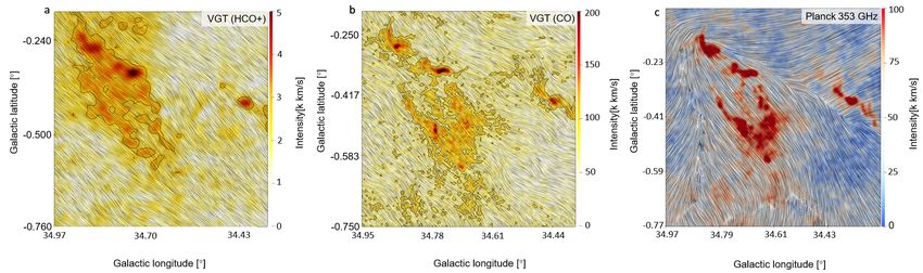
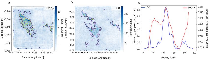
Magnetic Field towards the Supernovae Remnant W44 3
(LV99; Yuen & Lazarian 2020): magnetic fields, are introduced:
 
 ⊥ 1/3 1/3 ∑︁
 ,⊥ = ( ) ( , ) = 
 ℎ ( , ) cos(2 ( , ))
 
 (4) =1
 ,⊥ 1/3 ⊥ −2/3 
∇ ∝ ≈ ( ) ∑︁
 ⊥ ( , ) = 
 ℎ ( , ) sin(2 ( , )) (8)
 =1
where corresponds to the injection velocity. As an indicator
 1 
of ansiotropy, the gradient points to the direction with maximum = tan−1 ( )
variation of velocity fluctuation’s amplitude, which is perpendicular 2 
to the local magnetic field direction. where donates the pseudo polarization angle, and thus the POS
 The discussion of MHD turbulence above deals with sub-Alvénic magnetic field direction is defined as = + /2, as the same
turbulence, i.e., with the injection velocity of turbulence is statistics introduced in Sec. 2 about the Planck polarization.
less than the Alfvén velocity . For SNRs, the hydro effect is The relative orientation between the two magnetic field directions
significant and the turbulence is usually super-Alfvénic, i.e., with probed with the Planck polarization ( ) and the gradients ( ) is
 = / > 1. For such turbulence, the motions at the injection measured with the Alignment Measure (AM; González-Casanova &
scale are hydrodynamic due to the relatively weak backreaction of the Lazarian 2017), defined as
magnetic field. However, as the kinetic energy of turbulent motions
 1
follows the nearly isotropic Kolmogorov cascade, i.e., ∼ 1/3 , = 2(hcos2 ( )i − ) (9)
 2
the importance of magnetic backreaction gets stronger at smaller
scales. Eventually, at the scale = −3 , the turbulent velocity the theta angle is defined as = | − |. AM is a relative scale
becomes equal to the Alfvén velocity (Lazarian 2006) showing the ranging from -1 to 1, with AM = 1 indicating that and being
GS95 anisotropic scaling relation. globally parallel, and AM = -1 denoting that the two are globally
 orthogonal.

3.1.2 The Recipe of VGT 3.2 SCOUSEPY

For this work, we employ specifically the Velocity Channel Gradients To explore the VGT’s potential in probing three dimensional POS
Technique (VChGs) as the primary analytical approach. The essence magnetic fields, we use the SCOUSEPY, a Python software based
of the VChGs is the thin velocity channel, mapped as ℎ( , ). on the Semi-automated multi-COmponent Universal Spectral-line
The statistics of the intensity fluctuations in PPV space and their fitting Engine (SCOUSE) proposed by Henshaw et al. (016a, 2019),
relations to the underlying statistics of turbulent velocity and density to decompose the spectrum to individual Gaussian components.
were firstly proposed by Lazarian & Pogosyan (2000). It suggests SCOUSEPY is designed for fitting a large number of spectro-
that velocity fluctuations dominates over density fluctuation when scopic data with a multi-stages procedure. The software firstly di-
the channel width is sufficiently thin. Specifically, a thin channel is vides the spatial data of the user-selected region into small areas,
defined as the following criteria: named Spectral Averaging Areas (SAAs), and outputs a spectrum
 √︃ averaged spatially for each of the SAAs. Users manually mark the
Δ < ( 2 ), thin channel intended spectral range of the data, then SCOUSEPY performs the
 √︃ (5) fitting procedures, which adopts the appropriate fitting algorithms
Δ ≥ ( 2 ), thick channel from multiple fitting profiles, including Gaussian, Voigt, Lorentzian,
 and hyperfine structure fitting. For our work in the SNR, SCOUSEPY
 √︁
where Δ is the channel width and ( 2 ) represents velocity dis- chooses the Gaussian method. The final result consists of the best-
persion calculated from velocity centroid. Accordingly, the VChGs fitting solutions of pixels and velocity components for the data. More
is calculated from: details can be found in Henshaw et al. (016a).
 In this work, we adopt SCOUSEPY to decompose the W44’s
5 ℎ ( , ) = ∗ ℎ ( , ) CO emission lines into four Gaussian components. We follow the
 (6)
5 ℎ ( , ) = ∗ ℎ ( , ) tolerance criteria proposed in Henshaw et al. (016a): (i) all detected
 components must have a brightness temperature greater than three
where 5 ℎ ( , ), 5 ℎ ( , ) denote the x, y components of the times the local noise level; (ii) each Gaussian component must have
gradients in the thin channel map; , are Sobel kernels for a FWHM line-width of at least one channel: (iii) for two Gaussian
probing pixelized gradient map ( , ), namely components to be considered distinguishable, they must be separated
 by at least half of the FWHM of the narrowest of the two. (iv) the
 5 ℎ ( , )
 ( , ) = tan−1 ( ) (7) size of SAAs is set to six.
 5 ℎ ( , )
 In this paper we follow the procedure of sub-block averaging in-
troduced in Yuen & Lazarian (017a). The map is divided into sub- 4 RESULTS
blocks and the Gaussian fitting to individual sub-blocks to derive
 4.1 The POS magnetic fields in W44
the most probable orientation of the gradients of the sub-blocks. For
each thin velocity channel, such an averaging method is employed; Fig. 1 displays the integrated intensity maps of the HCO+ (1-0) emis-
consequently, we acquire compiled gradient maps ( , ) of the sion line and the CO (3-2) line, as well as the respective intensity-
same number as the thin velocity channel ( ). The pseudo Stokes velocity spectrum. The contours outline the overall structure of the
parameters, similar to the essences of the Planck polarization-probed SNR molecular cloud above mean intensity. The molecular cloud

 MNRAS 000, 1–10 (2020)

4 Liu, Hu & Lazarian
 [t]

Figure 1. Panel a & b: the integrated intensity maps of the HCO+ (1-0) emission line (left) and the CO (3-2) line (right). The purple contour lines in the intensity
maps start from the value of mean intensity. Panel c: the intensity-velocity spectrum of HCO+ (1-0; red) and CO (3-2; blue).

 Physical Parameter Symbol/Definition Value Reference

 Velocity dispersion of shocked gas 6.8 km s−1 Ref.1
 Velocity dispersion of quiescent gas 2.3 km s−1 Ref.1
 H2 Volume number density 0 100 - 300 cm−3 Ref.2 & 5
 Magnetic field strength 70 Ref.2
 Mass of an H atom H 1.67×10−24 g Ref.3
 Mean molecular weight H2 2.8 Ref.3
 Injection scale √︃ 100.00 pc Ref.4
 3D turbulent velocity = 3( 2 − 2 ) 11.08 km s−1 Derived
 Volume mass density 0 = 0 √︁H2 H 3.34 ×10−23 g cm−3 Derived
 Alfvén velocity = / 4 0 5.27 - 9.13 km s−1 Derived
 Alfvén Mach number = / 1.21 - 2.10 Derived
 Transition scale = −3 10.80 - 56.00 pc Derived
 Beam resolution of CO 0.26 pc Derived
 Beam resolution of HCO+ + 0.32 pc Derived

Table 1. Physical parameters of the W44 SNRs. References:

 [t]

Figure 2. Visualization of magnetic fields towards the W44 SNRs using the Line Integral Convolution (LIC). The magnetic fields were inferred from Planck
353 GHz polarized dust emission (panel c) and VGT using CO (panel b) and HCO+ (panel a) emissions. VGT measurements are overlaid on corresponding
integrated intensity color maps.

MNRAS 000, 1–10 (2020)

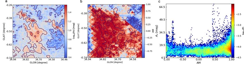
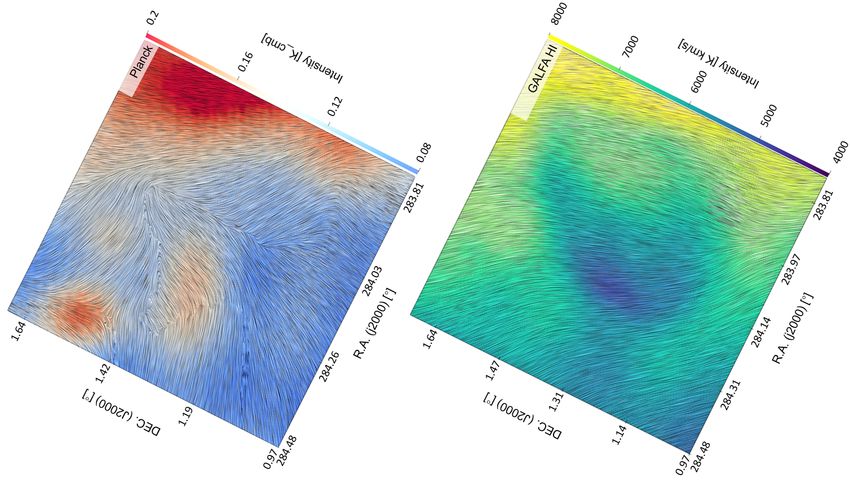
Magnetic Field towards the Supernovae Remnant W44 5
 [t]

Figure 3. Visualizations of the magnetic field orientation of the SNR foreground region probed with the Planck polarization ( , left panel) as well as with

the VGT on the GALFA H I emission ( , right panel). The graphs have been rotated (∼ 63◦ ) to convert the original equatorial coordinates to the galactic

coordinates.

 [t]

Figure 4. Panel a: the extinction map of the foreground H I emission. Panel b: the distribution of AM between the magnetic field orientations obtained by the
H I emission ( ) and the Planck polarization ( ). The purple contour lines in both maps mark the order of magnitudes of the optical extinction . The
 
graphs have been rotated (∼ 63◦ ) to convert the original equatorial coordinates to the galactic coordinates. Panel c: the -AM histogram of the H I emission.
P in the colorbar label indicates the percent of sampled data points of the two variables.

 MNRAS 000, 1–10 (2020)

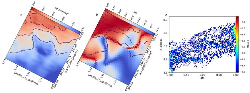
6 Liu, Hu & Lazarian
 [t]

Figure 5. Panel a: the extinction map of the CO (3-2) emission. Panel b: the distribution of AM between the magnetic field orientations obtained by the VGT
( 
 ) and the Planck polarization ( ). The purple contour lines in both maps mark the order of magnitudes of the optical extinction . Panel c: the
 -AM histogram of the CO (3-2) emission. P in the colorbar label indicates the percent of sampled data points of the two variables.

appears as filamentary elongating along the east-north direction. In dust in the foreground/background, VGT consequently results in a
particular, the velocity-intensity spectrum of the two gas lines indi- foreground/background magnetic field map.
cate three apparent velocity components at ≈ 10 km/s, 45 km/s, Fig. 3 presents the magnetic fields probed by VGT using H I, as
and 80 km/s. well as probed by the Planck polarization. Similarly, pixels, where
 As discussed in Sec.3, once the telescope resolves the SNRs at a the brightness temperature is less than three times the RMS noise
scale smaller than , we can expect the turbulence to be anisotropic level, are blanked out. We average the gradients over each 20×20
and velocity gradients are perpendicular to their local magnetic fields. pixels sub-block and smooth the gradients map with a Gaus-
 To calculate , we use several physical parameters of W44 from sian filter FWHM ≈ 10 0 . In the high-intensity regions, especially at
literature, which is summarized in Tab 1. The emission lines towards the top-north corner, the magnetic field orientations in both maps
W44 have beam resolution smaller than ≈ 10.80 - 56.00 pc. cohere with each other well. The Planck data is dominated by the
Therefore, the MHD turbulence in the SNR molecular cloud region foreground interference as the H I signals become the most intense in
is anisotropic, which fits the essential condition of applying the VGT. the areas. Near the W44, the intensity of the H I emission diminishes
 We then obtain the POS magnetic field map of the same region by to the minimum, so that the foreground’s contribution to the Planck
applying the VGT to both the CO and HCO+ emission data covering polarization is less significant.
all velocity components. Pixels where the brightness temperature We further quantitatively explore the foreground’s contribution by
is less than three times the RMS noise level are blanked out. We calculating hydrogen column density as well as the optical extinction
average the gradients over each 20×20 pixels sub-block and smooth , which is proportional to the number of grains along the LOS,
the gradients map with a Gaussian filter FWHM ≈ 3 0 . contributed by the W44 and the foreground/background. The hydro-
 The results are displayed in Fig. 2. We can see that the magnetic gen column density of the foreground/background is (Panopoulou
fields inferred from both CO and HCO+ are elongating along the et al. 2019):
filamentary intensity structures, showing insignificant variation. Ad- 
 = + 2 2 = 
ditionally, we make a comparison with the magnetic fields obtained ∫ (10)
from the Planck 353 GHz polarization data (see Fig. 2). Visually we = 1.823 × 1018 , cm−2 / (K km s−1 )
can see that in high-intensity regions, the magnetic field orientations 
in both the VGT maps and the Planck maps agree with each other where donates the column density of H I, 2 symbols the
well. However, in the low-intensity regions, in particular at the west- column density of 2 , and donates the brightness temperature of
north corner, the magnetic fields inferred from the VGT significantly H I emission. The hydrogen column density of W44 can be obtained
differ from the one acquired from the Planck polarization. Such a in a similar way using the the CO- 2 conversion factor =
phenomenon is further investigated in Fig. 3, where we look into the 2 − 4 × 1020 (we use 2 × 1020 in our calculation) in giant molecular
contribution of the polarized dust foreground, that potentially results clouds (Narayanan et al. 2011) :
in the inconsistency between the VGT and the Planck in low-intensity
 
regions. = + 2 2 = 2
 ∫ 
 −2 (11)
 = 2 ( 
 ), cm / (K km s−1 )
 
 where is the brightness temperature of CO emission. By adopt-
4.2 Contribution from the foreground 
 ing a linear relation between the hydrogen column density and optical
In Fig. 2, we observed misalignment between the magnetic field extinction (Güver & Özel 2009):
inferred from the VGT and Planck polarization. One possible con-
 = (2.21 ± 0.09) × 1021 (mag) (12)
tribution of the misalignment comes from the polarized dust fore-
ground, as well as background. To find the contribution, we adopt , we obtained the contributed by the W44 and the fore-
the neutral hydrogen H I emission line from the GALFA-H I survey ground/background, respectively. Fig. 4 and Fig. 5 display the results
to trace the magnetic field through VGT. As H I is well mixed with of such calculations.

MNRAS 000, 1–10 (2020)

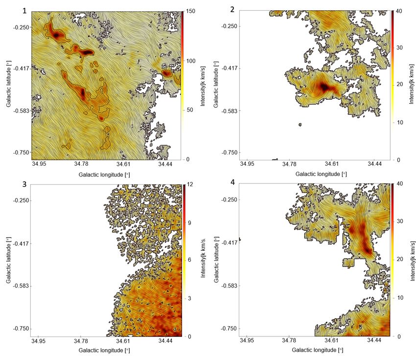
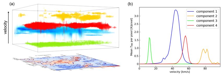
Magnetic Field towards the Supernovae Remnant W44 7
 [t]

Figure 6. Panel a: visualization of the decomposed components of the W44 SNRs at various velocities. Panel b: the velocity-intensity spectrum of different
Gaussian components.

 Fig. 4 quantitatively verifies the discussion about the foreground hierarchical and non-hierarchical components. Considering the fact
above. shows the peak significance in the top-north corner, where that both components contribute to VGT measurement, we further
the H i emission reaches the peak intensity, while in the W44 SNR combine them into the four most significant velocity components
regions and south-bottom region reaches the minimum, cohering based on the un-decomposed averaged spectral lines (see Fig. 1).
to the pattern discovered earlier in Fig. 3. The -AM histogram also
exhibits the positive correlation between the two variables that a large
 value corresponds to a large AM value as well, i.e. in regions As shown in Fig. 6, our final decomposed spectrum clusters is
where the H i emission is intense, the agreement between Planck dominated by 4 components. Panel b in Fig. 6 shows the spectrum
polarization and VGT measurement tend to be better. It implies a of the four major components. The blue curve with the highest in-
significant contribution from the foreground to the disagreement tensity peak shows the dominating component 1, with three other
seen in Fig. 2. components that are less significant. Note that because the velocity
 Fig. 5 shows the extinction map towards the SNR W44 obtained difference between each component is greater than their velocity dis-
from the CO emission line. Around the filamentary structure, persion, we expect these four components to be physical structures
displays the greatest magnitude ≥ 1.00 mag, which is greater than in real space.
the foreground’s ≤ 0.75. It indicates the dominance of W44’s
contribution in Planck so that we have a high consistency of the VGT- Fig. 7 displays the individual images of the velocity-wise magnetic
Planck. In the misalignment regions ( ≤ 0, west-north corners), field components. In general all components exhibit a magnetic field
 drops to ∼ 0.75 and the foreground’s increases to ∼ 0.8. orientation along the northeast direction. Component 1 (at ∼ 45
Therefore, the foreground has more contribution to the Planck in km s−1 ) exhibits the largest coverage of the filamentary SNR struc-
the region. The histogram similarly reveals the proportional correla- tures shown in Fig. 2, corresponding to the most prominent intensity
tion between and AM. The graphs thus confirm the association distribution in the Fig. 6 spectrum. The magnetic field orientations
between the foreground interference and the VGT-Planck inconsis- visually cohere with the overall magnetic field map in Fig. 2 in a
tency. highly consistent manner as well, indicating its dominating effect on
 the whole picture. It also shows agreement with Planck polarization
4.3 Magnetic field for various velocity components at high-intensity region. This can be easily understood based on the
 fact that component 1 has the most significant intensity so that its
We adopt the SCOUSEPY to decompose the W44 emission line into contribution dominates the projected magnetic field map, which is
various components. The decomposed spectrum is further processed contributed by all components.
by a hierarchical agglomerative clustering technique ACORNS (Ag-
glomerative Clustering for ORganising Nested Structures) 1 . We
perform the ACORNS clustering only on the most robust spectral The other three components have a smaller contribution to the
velocity components decomposed by SCOUSEPY, i.e. (i) the signal- SNR magnetic field overall, yet they reveal several details that are
to-noise ratio is greater than three; (ii) the minimum radius of a overwhelmed by the major regions with a high-intensity in compo-
cluster to be 30 00 , which is 150% of the beam resolution; (iii) for nent 1. Component 2 (at ∼ 80 km s−1 ) and 4 (at ∼ 50 km s−1 )
two data points to be classified as "linked", the absolute difference both indicate novel SNR structures that were not discovered initially
in measured velocity dispersion can be no greater 1.0 km/s. The in the complete image of the W44 magnetic field in Fig. 2. These
clustering comprises ∼ 97% of all data and results in a number of low-intensity regions have been hidden from the major high-intensity
 structures as in component 1 as well as the overall picture. Only by
 decomposing the magnetic field an inside individual investigation for
1 https://github.com/jdhenshaw/acorns. such concealed parts could be performed.

 MNRAS 000, 1–10 (2020)

8 Liu, Hu & Lazarian
 [t]

Figure 7. Visualizations of the four velocity-wise magnetic field components of the SNR W44, numbered as labeled. Magnetic fields are overlaid on corresponding
integrated intensity color maps of CO emission.

5 DISCUSSION et al. 2018a) and synchrotron polarization gradients (SPGs; Lazarian
 & Yuen 2018), as well as intensity gradients (IGs; Yuen & Lazarian
5.1 The range of VGT applications 2017; Hu et al. 2019). The theoretical justification of these tech-
 niques is similar to that of the VGT and it is routed in the theory
The VGT has been successfully used to study magnetic fields in
 of MHD turbulence and turbulent reconnection. In some cases, e.g.
diffuse H I (Yuen & Lazarian 017a; Hu et al. 2018, 2019, 020a; Lu
 while studying the magnetic fields in clusters of galaxies as in Hu
et al. 2020), molecular clouds, both in the galactic disk (Hu et al.
 et al. (2020b) we do not have the corresponding polarization data to
019a,b, 2021; Alina et al. 2020) and the Central Molecular Zone
 compare with. The present study shows that the measured gradients
(CMZ; Hu et al. 021c). This work shows that the VGT provides a
 arise mostly from turbulence and therefore can represent magnetic
useful tool for studying magnetic fields in supernovae remnants. The
 fields correctly in a wide variety of astrophysical conditions.
latter exhibit both shock regular compression and turbulence and
therefore it is obvious from the very beginning whether the VGT
could be accurate for them. However, our study has proven a good
 5.2 Prospects of the VGT
tracing power of the VGT in this setting.
 The present work also boosts our confidence in magnetic fields Probing magnetic fields in supernovae remnants (SNRs) is an es-
using other branches of the Gradient Technique, for instance, the sential yet technically challenging topic. Our research towards the
branches utilizing the synchrotron intensity gradient (SIGs; Lazarian SNR W44 magnetic field with the Velocity Gradients Technique

MNRAS 000, 1–10 (2020)

Magnetic Field towards the Supernovae Remnant W44 9
(VGT; González-Casanova & Lazarian 2017; Yuen & Lazarian 017a; (i) The SNR magnetic fields probed with the VGT generally agree well
Lazarian & Yuen 018a; Hu et al. 2018) has led to several intriguing with the results acquired with the Planck dust polarization, especially
discoveries. Quantitative studies verify the credibility of the VGT on in the high molecular gas emission intensity regions.
supernovae investigations. By comparing the W44’s magnetic field (ii) Using GALFA-HI data we evaluate the effect of the foreground on
probed with the VGT and the Planck 353 GHz dust polarization, the Planck polarization. We find that the discrepancy between the
shown in Fig. 2, we preliminary confirm the high consistency on Planck and the VGT arises due to the contribution the foreground.
the measurements by the novel VGT and the commonly-recognized Therefore, unlike Planck polarization, the VGT provides a better
Planck polarization. In other regions with a less intense gas emis- measure of the magnetic field in the supernovae remnant.
sion, we obtain evidence, in Fig. 3, Fig. 4, Fig. 5, indicating that the (iii) We decompose the SNR W44 into four individual components at
VGT-Planck consistency is affected by the foreground interference on various velocities using the Python implement SCOUSEPY and use
the Planck polarization data. The advantages of the VGT in remov- VGT to trace the magnetic field associated with different components.
ing the foreground interference have once again been highlighted (iv) We show that W44’s velocity component 1 at ∼ 45 km s−1
as in previous research (Hu et al. 020a; Lu et al. 2020). Further- exhibits the largest coverage of the filamentary SNR structures and
more, grouping the VGT-probed results intensity-wise as such helps gives best agreement with Planck polarization in terms of magnetic
to specify the most ideal conditions for applying the novel technique field orientation.
in SNR magnetic field tracing. (v) We verify the VGT’s potential in tracing the magnetic fields of the
 Meanwhile, compared to the general magnetic field probing ap- decomposed individual velocity components. We show the ability of
proach like the Planck dust polarization, the VGT possesses multiple VGT to measure three-dimensional magnetic field tomography.
advantages in tracing magnetic fields in SNRs. Along with the ca-
 The study verifies the credibility of the VGT on the SNR magnetic
pability of removing the foreground interference as stated above, the
 field tracing and reveals the potential of the novel technique for
technique also exhibits potentials in decomposing the SNR magnetic
 highly disturbed region. It also shows prospects for the technique
field into various components with different velocities and perform-
 for future application including tomographic studies of the SNRs.
ing in-depth studies towards the components individually. The W44
 We expect more profound findings to be revealed using the novel
velocity-wise magnetic field components unfold noteworthy details.
 Velocity Gradients Technique.
Individual investigations on such components provide valuable in-
sights about certain SNR structures that were completely buried
under the prominent high-intensity regions in the initial magnetic
field tomography. We reasonably expect that more useful informa- ACKNOWLEDGEMENTS
tion about the SNR will be found by such a novel perspective of M.L. acknowledges the invaluable support and accompany by Liu’s
research. The significance of this potential should not be underes- family and close acquaintances. Y.H. acknowledges the support of
timated, as so far the VGT remains the sole magnetic field tracing the NASA TCAN 144AAG1967. A.L. acknowledges the support
technique that is capable of identifying such informative details. of the NSF grant AST 1715754 and NASA ATP AAH7546. We
 acknowledge the Nobeyama Observatory for providing the data of
5.3 Prospective for cosmic rays’ study the W44 region.

The diffusion of cosmic rays (CRs) is a fundamental ingredient of as-
trophysics and has a broad impact on diverse astrophysical problems. DATA AVAILABILITY
Theoretically, the recent development of MHD turbulence theories
since GS95 and LV99 has brought a significant shift to the physical The data underlying this article will be shared on reasonable request
picture of CR diffusion (Yan & Lazarian 2002, 2004, 2008; Xu & Yan to the corresponding author.
2013; Lazarian & Yan 2014). It reveals that the CR diffusion and the
diffusion coefficient have a strong dependence on the properties of
MHD turbulence, i.e., the sonic Mach number and Alfvén Mach REFERENCES
number . Consequently, in the molecular cloud that SNRs interact
 Alina D., et al., 2020, arXiv e-prints, p. arXiv:2007.15344
with, the properties of the highly compressive and also magnetized
 Andersson M., Grumer J., Ryde N., Blackwell-Whitehead R., Hutton R.,
turbulence determine the diffusion of CRs that are accelerated by
 Zou Y., Jonsson P., Brage T., 2015, VizieR Online Data Catalog, p.
SNRs. J/ApJS/216/2
 The two important quantities and are also accessible by Armstrong J. W., Rickett B. J., Spangler S. R., 1995, ApJ, 443, 209
VGT. The dispersion of velocity gradient’s orientation reveals Bell A. R., 1978, MNRAS, 182, 147
(Lazarian et al. 2018b) and the amplitude of velocity gradient outputs Caprioli D., Spitkovsky A., 2014, ApJ, 783, 91
 (Yuen & Lazarian 020a). The application of VGT provides an Cho J., Vishniac E. T., 2000, ApJ, 539, 273
important observational test of fundamental theories of CR diffusion. Clemens D. P., Cashman L. R., Hoq S., Montgomery J., Pavel M. D., 2013,
 in American Astronomical Society Meeting Abstracts #221. p. 352.15
 Clemens D. P., Pinnick A. F., Pavel M. D., 2012a, ApJS, 200, 20
 Clemens D. P., Pavel M. D., Cashman L. R., 2012b, ApJS, 200, 21
6 CONCLUSION Elmegreen B. G., Scalo J., 2004, ARA&A, 42, 211
 Goldreich P., Sridhar S., 1995, ApJ, 438, 763
Tracing 3D magnetic fields in the molecular cloud that SNRs interact
 González-Casanova D. F., Lazarian A., 2017, ApJ, 835, 41
with is still obscured. In this work, we target the SNR W44 to test González-Casanova D. F., Lazarian A., 2019, ApJ, 874, 25
the VGT’s applicability in probing 3D magnetic fields. We employ Güver T., Özel F., 2009, MNRAS, 400, 2050
several data sets, including CO, HCO+ , and H I emission lines, as Harrus I. M., Hughes J. P., Singh K. P., Koyama K., Asaoka I., 1997, ApJ,
well as dust polarization data from Planck 353 GHz measurement. 488, 781
Our main discoveries are: Heiles C., 2000, AJ, 119, 923

 MNRAS 000, 1–10 (2020)

10 Liu, Hu & Lazarian
Henshaw J. D., et al., 2019, MNRAS, 485, 2457
Henshaw J. D., et al., 2016a, MNRAS, 457, 2675
Hu Y., Yuen K. H., Lazarian A., 2018, MNRAS, 480, 1333
Hu Y., Yuen K. H., Lazarian A., 2019, ApJ, 886, 17
Hu Y., Lazarian A., Yuen K. H., 2020a, ApJ, 897, 123
Hu Y., Lazarian A., Li Y., Zhuravleva I., Gendron-Marsolais M.-L., 2020b,
 ApJ, 901, 162
Hu Y., Lazarian A., Stanimirović S., 2021, ApJ, 912, 2
Hu Y., et al., 2019a, Nature Astronomy, 3, 776
Hu Y., Yuen K. H., Lazarian A., Fissel L. M., Jones P. A., Cunningham M. R.,
 2019b, ApJ, 884, 137
Hu Y., Yuen K. H., Lazarian A., 2020a, ApJ, 888, 96
Hu Y., Lazarian A., Wang Q. D., 2021c, arXiv e-prints, p. arXiv:2105.03605
Jokipii J. R., 1966, ApJ, 146, 480
Krucker S., Fivian M. D., Lin R. P., 2005, Advances in Space Research, 35,
 1707
Larson R. B., 1981, MNRAS, 194, 809
Lazarian A., 2006, ApJ, 645, L25
Lazarian A., 2007, J. Quant. Spectrosc. Radiative Transfer, 106, 225
Lazarian A., Pogosyan D., 2000, ApJ, 537, 720
Lazarian A., Vishniac E. T., 1999, ApJ, 517, 700
Lazarian A., Yan H., 2014, ApJ, 784, 38
Lazarian A., Yuen K. H., 2018, ApJ, 865, 59
Lazarian A., Yuen K. H., 2018a, ApJ, 853, 96
Lazarian A., Yuen K. H., Lee H., Cho J., 2018a, ApJ, 855, 72
Lazarian A., Yuen K. H., Ho K. W., Chen J., Lazarian V., Lu Z., Yang B., Hu
 Y., 2018b, ApJ, 865, 46
Lazarian A., Eyink G. L., Jafari A., Kowal G., Li H., Xu S., Vishniac E. T.,
 2020, Physics of Plasmas, 27, 012305
Lu Z., Lazarian A., Pogosyan D., 2020, MNRAS, 496, 2868
Mac Low M.-M., Klessen R. S., 2004, Reviews of Modern Physics, 76, 125
McKee C. F., Ostriker E. C., 2007, ARA&A, 45, 565
Mestel L., Spitzer L. J., 1956, MNRAS, 116, 503
Narayanan D., Krumholz M., Ostriker E. C., Hernquist L., 2011, MNRAS,
 418, 664
Panopoulou G. V., et al., 2019, ApJ, 872, 56
Peek J. E. G., et al., 2018, ApJS, 234, 2
Peek J. E. G., et al., 2011a, ApJS, 194, 20
Planck Collaboration et al., 2016, A&A, 594, A25
Planck Collaboration et al., 2020, A&A, 641, A12
Sashida T., Oka T., Tanaka K., Aono K., Matsumura S., Nagai M., Seta M.,
 2013, ApJ, 774, 10
Schmidt M., 1959, ApJ, 129, 243
Smith A., Jones L. R., Watson M. G., Willingale R., Wood N., Seward F. D.,
 1985, MNRAS, 217, 99
Xiao L., Fürst E., Reich W., Han J. L., 2008, A&A, 482, 783
Xiao L., Reich W., Fürst E., Han J. L., 2009, A&A, 503, 827
Xu S., Yan H., 2013, ApJ, 779, 140
Yan H., Lazarian A., 2002, Phys. Rev. Lett., 89, 281102
Yan H., Lazarian A., 2004, ApJ, 614, 757
Yan H., Lazarian A., 2008, ApJ, 673, 942
Yuen K. H., Lazarian A., 2017, arXiv e-prints, p. arXiv:1703.03026
Yuen K. H., Lazarian A., 2020, ApJ, 898, 66
Yuen K. H., Lazarian A., 2017a, ApJ, 837, L24
Yuen K. H., Lazarian A., 2020a, ApJ, 898, 65

This paper has been typeset from a TEX/LATEX file prepared by the author.

MNRAS 000, 1–10 (2020)