Using Machine Learning techniques to understand glucose fluctuation in response to breathing signals - Nikolaos Karamichalis
←
→
Page content transcription
If your browser does not render page correctly, please read the page content below

Using Machine Learning techniques
to understand glucose fluctuation in
    response to breathing signals

                  Nikolaos Karamichalis

             Master Programme in Data Science
                           2021

                    Luleå University of Technology
     Department of Computer Science, Electrical and Space Engineering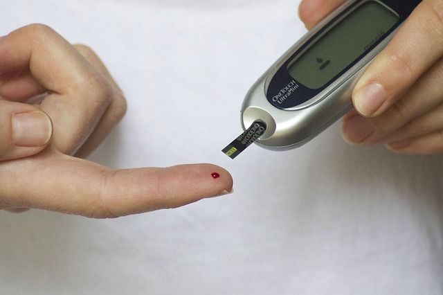
Abstract

Blood glucose (BG) prediction and classification plays big role in diabetic patients’ daily
lives. Based on International Diabetes Federation (IDF) in 2019, 463 million people are
diabetic globally and the projection by 2045 is that the number will rise to 700 million
people. Continuous glucose monitor (CGM) systems assist diabetic patients daily, by
alerting them about their BG levels fluctuations continuously. The history of CGM sys-
tems started in 1999, when the Food and Drug Administration (FDA) approved the first
CGM system, until nowadays where the developments of the system’s accurate reading
and delay on reporting are continuously improving. CGM systems are key elements in
closed-loop systems, that are using BG monitoring in order to calculate and deliver with
the patient’s supervision the needed insulin to the patient automatically. Data quality
and the feature variation are essential for CGM systems, therefore many studies are being
conducted in order to support the developments and improvements of CGM systems and
diabetics daily lives. This thesis aims to show that physiological signals retrieved from
various sensors, can assist the classification and prediction of BG levels and more specifi-
cally that breathing rate can enhance the accuracy of CGM systems for diabetic patients
and also healthy individuals. The results showed that physiological data can improve
the accuracy of prediction and classification of BG levels and improve the performance
of CGM systems during classification and prediction tasks. Finally, future improvements
could include the use of predictive horizon (PH) regarding the data and also the selection
and use of di↵erent models.

                                             ii
Contents
Chapter 1 – Literature review 5
1.1 Blood glucose prediction and machine learning applications . . . . . . . . 5
1.2 Machine learning prediction models and variety of inputs . . . . . . . . . 9
1.3 Limitations, data quality and improvement possibilities . . . . . . . . . . 11
1.4 Synthesis . . . . . . . . . . . . . . . . . . . . . . . . . . . . . . . . . . . . 13
Chapter 2 – Methodology 14
2.1 Methodologies comparison . . . . . . . . . . . . . . . . . . . . . . . . . . 14
2.2 Method CRISP-DM . . . . . . . . . . . . . . . . . . . . . . . . . . . . . . 15
2.3 Phases . . . . . . . . . . . . . . . . . . . . . . . . . . . . . . . . . . . . . 15
Chapter 3 – Empirical results 17
3.1 Business understanding . . . . . . . . . . . . . . . . . . . . . . . . . . . . 17
3.2 Data understanding . . . . . . . . . . . . . . . . . . . . . . . . . . . . . . 18
3.3 Data preparation . . . . . . . . . . . . . . . . . . . . . . . . . . . . . . . 22
3.4 Modelling research . . . . . . . . . . . . . . . . . . . . . . . . . . . . . . 22
3.5 Evaluation . . . . . . . . . . . . . . . . . . . . . . . . . . . . . . . . . . . 27
3.6 Deployment . . . . . . . . . . . . . . . . . . . . . . . . . . . . . . . . . . 34
Chapter 4 – Analysis of results 35
4.1 Data correlation . . . . . . . . . . . . . . . . . . . . . . . . . . . . . . . . 35
4.2 Comparison with the literature . . . . . . . . . . . . . . . . . . . . . . . 37
Chapter 5 – Conclusion 39
References 40
Appendices 43
iiiAcknowledgments
I would like to thank my supervisor professor Ahmed Elragal for the support and the
guidance during this thesis project, my family and my girlfriend for supporting me during
this period and their mental assistance.
Luleå, September 2021
Nikolaos Karamichalis
1List of figures
1.1 Self-monitoring of blood glucose with a glucometer. . . . . . . . . . . . . 6
1.2 Single use insulin pens. . . . . . . . . . . . . . . . . . . . . . . . . . . . . 7
1.3 Complete set for blood glucose measurement. Glucometer, lancing device,
strips and lancets. . . . . . . . . . . . . . . . . . . . . . . . . . . . . . . . 8
1.4 Example of an insulin pump, connected to a diabetic patient. . . . . . . . 9
1.5 Data reporting dashboard on a screen. . . . . . . . . . . . . . . . . . . . 11
1.6 Wearable smart watch, monitoring personal data. . . . . . . . . . . . . . 12
3.1 Principle Component Analysis (PCA) components for diabetic patients. . 23
3.2 Principle Component Analysis (PCA) components for healthy patients. . 24
3.3 Logistic regression model. . . . . . . . . . . . . . . . . . . . . . . . . . . 24
3.4 Random forest model. . . . . . . . . . . . . . . . . . . . . . . . . . . . . 25
3.5 Decision Tree model. . . . . . . . . . . . . . . . . . . . . . . . . . . . . . 25
3.6 Support Vector Machine Classification model, linear kernel. . . . . . . . . 25
3.7 Support Vector Machine Classification model, polynomial kernel. . . . . . 25
3.8 Support Vector Machine Classification model, radial basis function kernel. 26
3.9 Support Vector Machine Classification model, Sigmoid kernel. . . . . . . 26
3.10 Diabetic subset, Logistic Regression Classification report. . . . . . . . . . 27
3.11 Diabetic subset, Random Forest Classification report. . . . . . . . . . . . 28
3.12 Diabetic subset, Decision Tress Classification report. . . . . . . . . . . . 28
3.13 Diabetic subset, Support Vector Machine Classification, linear kernel Clas-
sification report. . . . . . . . . . . . . . . . . . . . . . . . . . . . . . . . . 29
3.14 Diabetic subset, Support Vector Machine Classification, polynomial kernel
Classification report. . . . . . . . . . . . . . . . . . . . . . . . . . . . . . 29
3.15 Diabetic subset, Support Vector Machine Classification, RBF kernel Clas-
sification report. . . . . . . . . . . . . . . . . . . . . . . . . . . . . . . . . 30
3.16 Diabetic subset, Support Vector Machine Classification, Sigmoid kernel
Classification report. . . . . . . . . . . . . . . . . . . . . . . . . . . . . . 30
3.17 Diabetic subset, overall accuracy. . . . . . . . . . . . . . . . . . . . . . . 30
3.18 Healthy subset, Logistic Regression Classification report. . . . . . . . . . 31
3.19 Healthy subset, Random Forest Classification report. . . . . . . . . . . . 31
3.20 Healthy subset, Decision Tress Classification report. . . . . . . . . . . . . 32
3.21 Healthy subset, Support Vector Machine Classification, linear kernel Clas-
sification report. . . . . . . . . . . . . . . . . . . . . . . . . . . . . . . . . 32
3.22 Healthy subset, Support Vector Machine Classification, polynomial kernel
Classification report. . . . . . . . . . . . . . . . . . . . . . . . . . . . . . 33
23.23 Healthy subset, Support Vector Machine Classification, RBF kernel Clas-
sification report. . . . . . . . . . . . . . . . . . . . . . . . . . . . . . . . . 33
3.24 Healthy subset, Support Vector Machine Classification, Sigmoid kernel
Classification report. . . . . . . . . . . . . . . . . . . . . . . . . . . . . . 34
3.25 Healthy subset, overall accuracy. . . . . . . . . . . . . . . . . . . . . . . . 34
4.1 Variable correlations for diabetic patients. . . . . . . . . . . . . . . . . . 36
4.2 Variable correlations for healthy individuals. . . . . . . . . . . . . . . . . 37
3List of tables
3.1 Healthy individuals statistics table . . . . . . . . . . . . . . . . . . . . . 19
3.2 Diabetic patients statistics table . . . . . . . . . . . . . . . . . . . . . . . 19
3.3 Selected dataset attributes . . . . . . . . . . . . . . . . . . . . . . . . . . 19
3.4 Healthy subset demographic information . . . . . . . . . . . . . . . . . . 20
3.5 Diabetic subset demographic information . . . . . . . . . . . . . . . . . . 21
3.6 Blood glucose levels boundaries . . . . . . . . . . . . . . . . . . . . . . . 22
5.1 Dataset attributes . . . . . . . . . . . . . . . . . . . . . . . . . . . . . . . 44
4Chapter 1
Literature review
1.1 Blood glucose prediction and machine learning
applications
Diabetes Type 1 patients have to continuously monitor their blood glucose (BG) levels,
in order to calculate the amount of insulin doses they have to inject to themselves. BG
levels have to be under control and remain under specified healthy ranges in order to
avoid complications. Machine learning techniques can be used for BG classification and
prediction for Type 1 diabetic patients, to control the BG levels under the required lim-
its. In order for health care sta↵ to evaluate each diabetic person’s BG levels over time,
hemoglobin A1c (HbA1c) test is used. The report of Little, Randie R. et al. (2009) [1],
mentions that HbA1c test measures the amount of BG levels attached to hemoglobins
and can represent a monitoring of 8–12 weeks, based on the erythrocytes circulation,
therefore, HbA1c tests are integral to the management of individuals with diabetes.
The goal of each diabetic patient is to keep their BG levels within healthy limits,
which di↵er for each patient and are being set in collaboration with their doctors. When
the BG levels are higher than the limit, the event is called hyperglycaemia and when are
lower, the event is called hypoglycaemia. In order for each patient to control their BG
levels, they should prevent these events, that’s why machine learning techniques can be
used to predict BG levels and alert the patients before the occurrence of these events.
In order for diabetic patients to measure glucose levels in their blood, they can self-
monitor BG levels, which gives a discrete overview of the measurements each time, but
not the trend and fluctuations of BG levels. The use of Continuous Glucose Monitoring
(CGM) systems which continuously check the BG levels supports the monitoring by col-
lecting data over time for each patient during their daily lives. This can then be used as
input for machine learning applications. CGM systems overpass the discrete limitations
of self-monitoring BG levels with glucometers as Gross et. al (2000) outline [2].
51.1. Blood glucose prediction and machine learning applications 6
Figure 1.1: Self-monitoring of blood glucose with a glucometer.
The report of Klono↵ et. Al (2017) [3] contains a review about CGM systems, the
technology used and their impact on clinical use. Comparing self-monitor BG (SMBG)
and CGM systems, the report points out that on average a CGM system is generating
288 measurements per day whereas SMBG requires patient initiative to generate a mea-
surement, hence measurements rarely exceed 7 measurements in total per day. Moreover
CGM systems can monitor the trend of BG levels, can provide information about the
direction and rate of changing of BG levels and also alert the patient about the trend of
the glucose in order to avoid hyperglycemias and hypoglycemias.
One disadvantage of CGM systems comparing to SMBG outlines in the review is that
CGM systems are more prone to generate outlier data and for that reason, CGM systems
were previously approved and used in addition to SMBG and not as stand alone solution.
Patients were using SMBG in order to calibrate the data of CGM systems, by verifying
the CGM data. Although this changed after December 2016, when the FDA (Food and
Drug Administration) approved the first CGM system where treatment decisions could
be based only to the CGM system without compulsory use of SMBG.
Langendam et al. (2012) [4] also could show that CGM systems can be used as sensors
for CGM augmented insulin pump therapy, which, compared to patients using SMBG
and multiple daily injections of insulin (MDI) had a significant reduce on HbA1c level in
a period of six months.1.1. Blood glucose prediction and machine learning applications 7
Figure 1.2: Single use insulin pens.
An example of using Machine learning techniques for BG classification and prediction,
could be the research of Kevin Plis et al. (2014) [5], where a Support Vector Regression
(SVR) model was used in order to predict BG levels, more specifically, hypoglycaemia.
The model achieved 23% better accuracy when it came to BG levels prediction compared
to diabetes experts predicting hypoglycaemic events 30 minutes beforehand.
Machine learning applications are being used in order to predict the BG levels, al-
though a universal model is not yet created since each patient’s case is dependent on
many factors and can be quite personalised as mentioned in Woldaregay et al. (2019) [6].
The publication mentions that the monitoring and analysis of personal data via mobile
health applications (mHealth apps), sensors, wearables, and other point of care (POC)
devices for self-monitoring and management purposes have created opportunities to train
the machine learning models in a better and more efficient way.1.1. Blood glucose prediction and machine learning applications 8
Figure 1.3: Complete set for blood glucose measurement. Glucometer, lancing device, strips
and lancets.
The BG level ranges di↵er between healthy individuals and diabetic patients and es-
pecially in diabetic patients, i.e. glucose fluctuations of diabetics are larger compared
to healthy individuals. Based on American Diabetes Association’s report (2021) [7], the
normal target range of BG levels for diabetic type 1 patients and CGM readings is be-
tween 3.9 mmol/L to 10.0 mmol/L. For healthy individuals, BG levels between 4 mmol/L
and 7.5 mmol/L are considered normal, as per international guidelines [8].
Glucose fluctuation for diabetic patients can result in events of hyperglycaemia or
hypoglycaemia. These events are connected with potential risks and implications for
diabetic patients, like possible vascular damage and severe hypoglycaemias, as outlined
in the report of Ceriello et al. (2018) [9].
The use of supervised machine learning models can improve the prediction of BG
levels, by significantly minimising the false positive alerts of hypoglycaemia and hyper-
glycaemia events, as shown in Marcus et al. (2020) [10].
The evolution of the performance levels of many machine learning models and the
larger availability of the data, lead to study results, like Yonit Marcus et. al (2020)
[10], where a new personalised supervised machine learning method was developed that
outperformed previous results on BG level prediction. This continuous improvement of
the BG levels prediction can also improve the accuracy of current and future closed-loop
‘artificial pancreas’ systems as is mentioned in the publication.
A closed-loop Artificial Pancreas (AP) system is capable of automatic information
collection, decision making and insulin management which includes supervised, semi-1.2. Machine learning prediction models and variety of inputs 9
supervised and unsupervised methods. The automatic collection of information can be
for example through CGM systems that monitor the BG levels, through wearable sen-
sors that monitor the Heart rate, amongst others. Then these variable are used as input
for the decision making algorithms which, then again, enable the output the system to
regulate the dosage on insulin inputs for each patient.
Figure 1.4: Example of an insulin pump, connected to a diabetic patient.
The study of Cinar (2017) [11], shows that a fully automated AP system can function
without any manual information, through the collection of multi-variable inputs. These
inputs are collected through wearable devices and CGM systems and help the used mod-
els to adapt to the changes of each state of the user. This then leads to performance
assessment, fault detection and diagnosis, machine learning and classification to the AP
systems in order to understand various input signals, which would lead to a fully auto-
mated, multi-variable AP systems.
1.2 Machine learning prediction models and variety
of inputs
BG levels can be directly a↵ected by multiple factors, such as, the history of BG values,
insulin dosages, physical activity, and carbohydrates intake. Also, factors like body mass
index, stress level, amount of sleep, illnesses, medications, smoking, menstruation, alco-
holism, allergies, and altitude can a↵ect the glucose levels in an individual’s blood.1.2. Machine learning prediction models and variety of inputs 10
Moreover, the predictive performance metrics of a model can be a↵ected by many tech-
nical factors, apart from the factors that a↵ect BG levels, such as the type of machine
learning, data size, prediction horizon (PH), validation approaches, etc. as mentioned in
Woldaregay et al. (2019) [6]. The results of the research also outline that there are no
studies assessing model predictive performance during stress and infection incidences in
a free-living condition.
The D1NAMO dataset of Dubosson et al. (2018) [12], contains BG levels, collected
from CGM devices and also data monitored through wearable sensors such as, electro-
cardiogram (ECG signals), breathing signals, accelerometer outputs and annotated food
pictures, collected from nine diabetic type 1 patients and twenty healthy individuals.
The publication also mentions that there are several open questions that need to be fur-
ther research, which on of them is that the availability of multiple signals could permit to
study relationships between them, more specifically the impact of BG levels on breathing
rate signals, if any and point out any possible relevant correlations among the data by
using di↵erent algorithms based on machine learning.
There are studies like Zarkogianni et al. (2015) that monitored ten diabetic type 1
patients for six days. The goal of the study was to assess and compare di↵erent glucose
prediction models for type 1 diabetic patients by monitoring their BG levels and physical
activity. The data were collected via a CGM system and a wearable body monitoring
system, which recorded the energy expenditure of daily physical activities or exercise
events [13].
The study of Rodrı́guez-Rodrı́guez et al. (2021) monitored 25 diabetic type 1 patients
for 14 days during their normal daily routines using CGM systems for their BG levels
and a wearable smart band that monitored their heart rate, physical activity (number
of steps) and their sleep data. The aim of the study was to compare feature selection
and forecasting for machine learning algorithms that are used for glycaemia prediction
of type 1 diabetic patients [14].1.3. Limitations, data quality and improvement possibilities 11
Figure 1.5: Data reporting dashboard on a screen.
Porumb et al (2020) [15] study, monitored eight healthy individuals, but only included
four of them in the final analysis. The researchers collected actigraphy, ECG signals and
BG levels recordings using commercial wearable sensors, between eight and fourteen days.
The aim of the study was to detect low BG levels in healthy individuals based on the
ECG signals and actigraphy, monitored during normal periods of fourteen nights.
Xie, J. et al (2020) paper [16], bench-marked machine learning regression models,
vanilla Long-Short-Term-Memory (LSTM) network and Temporal Convolution Network
(TCN) network, against the classical Autoregression with Exogenous inputs (ARX)
model. The results indicated that the ARX model, achieved the lowest average Root
Mean Square Error (RMSE) in 30-minutes predictive horizon (PH). Compared to the
deep neural networks, comparing ARX to TCN model, showed that ARX model was
prone to over predictions and under predictions of BG levels, while the prediction per-
formance of the vanilla LSTM network was stable.
1.3 Limitations, data quality and improvement pos-
sibilities
Woldaregay et al. (2019) mentions that di↵erent input parameters a↵ect the predictive
performance of the used models that can lead to the main limitation, which is the lack of
well-defined data attributes and directly dependant on manual reporting by the individual
users, like carbohydrate intake, making them prone to errors. Moreover, the publication
mentions that the there are many limitations on estimation and quantification of the ap-
proximate e↵ect of physical activities, stress, and infection incidence on the BG levels [6].1.3. Limitations, data quality and improvement possibilities 12
The results of the study of Rodrı́guez-Rodrı́guez et al. (2021) mention that D1NAMO
dataset from [12], which monitored twenty healthy individuals and nine diabetic type 1
patients, recording their electrocardiograms, breathing, accelerometer signals and BG
levels, can improve the accuracy of the glycaemia prediction and extending the PH,
which would help to provide early warning of health monitoring.
Figure 1.6: Wearable smart watch, monitoring personal data.
Dash et al. (2019) [17] provide an overview of diabetes detection using ECG signals,
whereas Mackay et al. (1983) [18] only measured heart rate variation at di↵erent levels
of breathing modes for healthy and diabetic patients.
The study of Porumb et al. (2020) [15] used artificial Intelligence (AI) to detect noc-
turnal hypoglycaemic events using ECG by monitoring 24 hours for 14 days in 8 healthy
individuals. The limitations that the report mentioned were firstly that additional tests
should take place in the future focusing on diabetic patients and more than 8 individuals.
Secondly, the performance of the model could be improved by including more physiologi-
cal signals that might be correlated with the BG levels variations, such as activity levels,
temperature, skin conductivity or nutrition information. Last, a dataset with diabetic
patients could include also SMBG information, therefore the system could continuously
learn from new data.1.4 Synthesis
Based on the literature review, many publications took under consideration the assess-
ment of machine learning techniques and models for prediction and classification. Also,
the used various performance metrics in order to evaluate the performance of the used
models.
The most commonly used and best performed models, were the Random forest (RF)
and the Support vector machine (SVM), where in some cases Decision tree (DT) model
was used along with the RF model, although the performance metrics showed that usu-
ally DT model performed worse than the RF. There were various kernel functions used
in many cases along with the models, that’s why di↵erent kernel functions were used
with the SVM model. Regarding regression, Support vector regression (SVR) and linear
regression model were commonly used. Since the variables of the current dataset are not
continuous, but categorical, logistic regression (LR) model was considered instead of the
linear regression model. More specifically, the desired classification output of the target
feature was not binary but three categories were considered, the multinomial extension
of the LR model was used.
RF and DT models were selected since they perform well with non-linear data, with
large datasets and they are dealing well with outliers. Although, DT is more prone to
overfitting than RF, it cannot result always to optimal trees, but is faster than RF. SVM
model is performing well with multiple dimensions, but it results to high training time
with large datasets. LR performs well with large non-linear data and supports multino-
mial regression, on the other hand is prone to overfitting and cannot handle missing data.
Regarding the performance metrics, the use of the Root Mean Squared Error (RMSE)
and the accuracy of the evaluated models was very common, often using the precision,
recall and f1 score as extra metrics as well. Therefore RMSE and classification report
were taken under consideration, including also the Mean absolute error (MAE) and the
Mean squared error (MSE) as performance metrics.
13Chapter 2
Methodology
2.1 Methodologies comparison
There are several ways and approaches that were compared in order to find the best
option to investigate the stated problem.
Sample, Explore, Modify, Model, and Assess (SEMMA) is one approach used as data
mining methodology. SEMMA includes five phases, where the first phase includes the
data sampling, next the understanding of the data, data modification, model selection
and last the assessment.
The second methodology, Knowledge Discovery in Databases(KDD) is a process that
is used to find knowledge in data and is also used as data mining methodology. KDD
contains five phases as well, first the selection phase, where the selection of the features
in the dataset is performed. Then the pre-processing, where the pre-processing of the
data is taking place. Next, the transformation phase, which includes the data transfor-
mation with di↵erent methods. The the data mining phase, which includes the search
for interesting patterns connected with data mining focus and last the evaluation, where
the evaluation of the selected patterns takes place.
The Cross-industry standard process for data mining, also know as CRISP-DM, which
is the most widely-used methodology, contains six phases. Comparing CRISP-DM and
the previous two methodologies, one big advantage of CRISP-DM is that supports the
reverse transitions between its phases. This advantage can be helpful when dealing with
real data, because fixes on target data can be applied without finishing a whole cycle of
the phases. The CRISP-DM phases will be described below.
142.2. Method CRISP-DM 15 2.2 Method CRISP-DM We consider CRISP-DM the best methodology for this thesis, because is widely used in data science and predictive analytics projects. CRISP-DM is an open standard process model, created in 1996 and reconfigured on several occasions throughout the years, but still remains the leading methodology until today [19]. CRISP-DM divides the process into six phases, which are described below. 2.3 Phases 2.3.1 Business understanding The business understanding phase explains the goals and the accomplishments that aim to be achieved from a business perspective. To understand how the glucose levels of diabetic patients change in response of breathing signals will allow to shed light on the correlation between glucose changes alongside with breathing signals. This can then be used for prediction of glucose levels, breathing signals and their correlation. Also, it can be explored if there is a dependency between them. 2.3.2 Data understanding The data understanding phase explains the data that will be used as input after their initial collection, in order to get more familiar with it. Any data quality issues that might occur must be shown in this phase in order to be resolved. 2.3.3 Data preparation The data preparation phase resolves any data quality issues and prepares the data to its final state. In our case the preparation of the data includes attribute selection, data cleaning and also setting a common format when it comes to numerical and date-time data types. 2.3.4 Modelling research The modelling research phase includes the investigation and selection of models that fit the specific problem and produce the most optimal outcome. The selected models along with their outcomes will be assessed in the following phase.
2.3.5    Evaluation
The evaluation phase evaluates the selected models and their outcomes, including the
evaluation of requirement fulfilment. In this phase the optimal model is chosen based on
the evaluation.

2.3.6    Deployment
The deployment phase includes the organisation and representation after the evaluation
phase in order to be accessible to the target group, in our case the publication of the
final report.

                                          16
Chapter 3
Empirical results
In this chapter, the empirical results of the report will be presented based on CRISP-
DM methodology and phases in the same order as they were represented in the previous
chapter.
3.1 Business understanding
The first phase of the CRISP-DM methodology is the Business understanding phase,
where the aim of the report is going to be explained. The literature review outlines that
there is a need for data and analysis of data including multiple variables and more specif-
ically physiological signals, monitored under di↵erent circumstances and both including
healthy and diabetic individuals. These variables could then be used for classification
and prediction of the glucose levels in diabetic patients and therefore help them to avoid
events like hypoglycaemia and hyperglycaemia.
Di↵erent stakeholders can benefit, such as doctors and professionals working in the
health industry, as well as health insurance companies. Clinicians can benefit, by using
the data to calibrate better each patient’s diabetes monitoring and daily insulin dosages,
nutrition and physical exercise. This then results in a better monitoring of each patient’s
diabetic journey and control of their BG levels.
One crucial constraint is that currently, in order to create a dataset with CGM and
physiological signals, the patient will be required to wear two sensors, one for the BG
level monitoring and one for the physiological signals. Additionally, the patient will have
to note their insulin dosages manually, in cases that they are not using a closed-loop
insulin pump system. Beside that, the cost of the required sensors and their expendable
parts is high and currently there is no single sensor that can read both glucose levels and
physiological signals.
173.2. Data understanding 18
Current sensor technologies can always be improved in terms of calibration of the sen-
sors, their accuracy, as well as the lag between the sensor’s readings and the actual BG
levels. Also, the development of a joint sensor between CGM and physiological signals
might be considered as business goal for the healthcare industry.
3.2 Data understanding
3.2.1 Collection of initial data
The D1NAMO dataset of Dubosson et al. (2018) [12], was retrieved and used for model
building and analysis . It contains CGM data and physiological signals, collected from
nine diabetic type 1 patients and twenty healthy individuals. The whole dataset is open
access and can be downloaded.
3.2.2 Description of data
The dataset contains two subsets, the diabetic, which contains data from 9 type-1 di-
abetic patients and the healthy, which contains data from 20 individuals, but one of
them has diabetes type-1, hence it was dropped for the analysis, as he was considered as
outlier, but he is included in the data understanding phase. The diabetic individual was
included in the healthy subset initially, because he didn’t wear a CGM system like the
rest diabetic patients, therefore he followed the healthy subset protocol. The recordings
for the dataset were from 1st of October 2014 until 4th of October 2014.
Healthy individuals received instructions to wear a physiological sensor after waking
up in the morning, and remove tit before sleep for 4 days in a row. Beside the physio-
logical sensor, a glucose meter was given and explained to healthy individuals, in order
to preform 6 BG level measures per day, one before each meal and one 2 hours after the
meal. Also, they were taking pictures of their meals.
Diabetic patients participated upon agreement with their diabetologist and received
instructions for the data acquisition directly from their doctors. Same as healthy individ-
uals they were wearing the physiological sensor for 4 days and they were taking pictures
of their meals. Since they were using CGM systems, the BG levels have been acquired
from their CGM devices, that included BG measurements every 5 minutes.
Every individual has a numbered folder under every subset. Each healthy individual’s
folder contains:
• an annotation.csv file that reports any issue the individuals faced with their sensors;
• a folder that contains their meal pictures;3.2. Data understanding 19
• a food.csv file that contains each meal’s annotation;
• a glucose.csv file that includes their BG levels measurements and
• a folder that contains each day as subfolders and all of them contain each physio-
logical signal’s raw data and a date summary.csv file that includes the physiological
signals’ values per second.
The diabetic patients’ folders contained the same exact content as mentioned before,
but since they were monitoring the dosages of insulin they were injecting, they also
contained an extra csv file:
• an insulin.csv file that contains the fast and slow insulin dosages that the patient
injected per day.
Total Average per individual
Signals recording ⇠1100h ⇠55h
Glucose measurements 470 23.5
Table 3.1: Healthy individuals statistics table
Total Average per individual
Signals recording ⇠450h ⇠50h
Glucose measurements 8414 934.9
Table 3.2: Diabetic patients statistics table
The main focus was on glucose.csv, insulin.csv and the summary.csv file of physio-
logical signals, per day, sorted by date and time. Since not all the data are relevant to
blood glucose prediction and classification, only some attributes were selected. In the
table that can be found in Appendix A, all the available attributes are listed and marked
as selected or non-selected. The Table 3.3 contains the selected attributes.
Name Source Description Data type
date glucose.csv, insulin.csv The date of the input date (format: YYYY-MM-DD)
time glucose.csv, insulin.csv The time of the input time (format: hh:mm:ss)
Time summary.csv The date and time of the input datetime (format: YYYY-MM-DD hh:mm:ss.uu
glucose glucose.csv The blood glucose levels float
fast insulin insulin.csv The amount of fast acting insulin injected integer
slow insulin insulin.csv The amount of slow acting insulin injected integer
HR summary.csv The heart rate levels integer
BR summary.csv The breathing rate levels float
Activity summary.csv The activity levels float
Table 3.3: Selected dataset attributes3.2. Data understanding 20
The demographic information for both subsets is available in the report of the dataset,
all patients underwent anthropometric assessments including each patient’s Age, Gender,
Height (cm) and Weight (kg).
Healthy subset sorted by age:
Age Gender Height (cm) Weight (kg)
26 Woman 174 64
27 Man 184 7
28 Woman 170 54
29 Man 170 62
29 Man 190 83
31 Man 171 65
32 Woman 162 58
32 Man 170 72
32 Man 173 89
33 Man 170 78
33 Man 177 72
33 Man 185 90
33 Man 186 94
34 Woman 164 63
34 Man 185 87
34 Man 192 81
36 Man 170 73
36 Man 176 68
43 Man 176 74
45 Man 178 82
Table 3.4: Healthy subset demographic information3.2. Data understanding 21
Diabetic subset sorted by age:
Age Gender Height (cm) Weight (kg)
NA Man 180–189 80–89
20–29 Man 170–179 60–69
20–29 Man 180–189 70–79
20–29 Man 180–189 80–89
30–39 Man 180–189 80–89
30–39 Man 190–199 70–79
30–39 Woman 160–169 70–79
60–69 Woman 150–159 50–59
70–79 Woman 160–169 50–59
Table 3.5: Diabetic subset demographic information
3.2.3 Exploration of data
The data was collected from multiple sources categorized per individual. The common
attribute for each source was the data and time of the data report, where in the glu-
cose and insulin data sources the date and time are reported with the same format, but
in the case of the physiological data there is a single datetime attribute. The variable
consisted of date and time values reported into a single value and with a di↵erent format.
The glucose values were reported in the scale of mmol/l (millimoles per litre), which
is an international format for measuring the amount of concentrated glucose.
Insulin has an international unit of measurement, where 1 insulin unit contains 0.347
grams of crystalline insulin.
The heart rate is measured by beats per minute and ranges between 25-240, while
breathing rate is measured by breaths per minute and ranges between 4-70. Activity is
measured by Vector Magnitude Units, measured in g, as described in Zephyr’s official
data description of BioHarness 3 [20].
3.2.4 Verifying quality of data
Since the data for diabetic individuals was joined in every case based on the glucose
reports, there were cases that some values were missing, for example not every individ-
ual was injecting insulin per 5 minutes, while the glucose inputs were being reported
automatically from the CGM sensor every 5 minutes. In cases where merely the glucose
values were available, the data inputs were dropped.3.3. Data preparation 22
The healthy individuals were not injecting insulin, therefore, the data frame of insulin
was not present and the join on the data was made using the inner way, meaning that only
the cases that the datetime on the glucose and the physiological data frames were match-
ing. The same preprocessing of not available data was used for the healthy subset as well.
The final cases for the diabetic patients were 4065 data reports, and 381 data reports
for the healthy individuals.
3.3 Data preparation
The common attribute for each source was the data and time of the data report, therefore,
during data collection all date and time inputs were transformed to a single attribute
with the format YYYY-MM-DD hh:mm:ss and later the attributes of date and time were
dropped. In the cases that the datetime values, per source, were duplicated, the data
inputs were dropped and the last one was kept in the data frame.
The iterations run per individual and created three data frames for glucose, insulin
and physiological data. After collected all data per individual, since the focus was on
glucose levels, all three data frames were merged into a single one based on the glucose
date time reports, meaning that the non-matching inputs from the physiological data
and insulin data frames were dropped.
The final step was to append the data frames per individual into a single data frame
that was used for the analysis.
In order to classify the BG levels, the target feature, glucose class, was set. The class
was defined based on the glycaemic events, hypoglycaemia, normal and hyperglycaemia.
Since the boundaries di↵er between healthy diabetic patients, they were set di↵erently
as described in Table 3.4.
Hypoglycaemia Normal Hyperglycaemia
Diabetic patients < 3.9 3.9 - 10.0 > 10.0
Healthy individuals < 4.0 4.0 - 7.5 > 7.5
Table 3.6: Blood glucose levels boundaries
3.4 Modelling research
Based on the literature review and the structure of the data, the classifiers that were
trained and applied were Logistic Regression (LR), Random Forest (RF), Decision Tree
(DT) and Support Vector Machine (SVM) Classification, including all four available3.4. Modelling research 23
kernels (Linear, Polynomial, Radial basis function and Sigmoid).
Before using the data as input for each model, the data was split 80% to training
subset and 20% to testing subset. The split of the dataset helps to deal with large
datasets or when the training of a model is very time consuming by using the training
dataset to fit the model and the test dataset to evaluate the fit of the model. A desired
fit is when a model can correctly provide accurate outputs based on the input data.
The training subset was scaled, meaning that a common distance between the data
points was used, therefore the data were standarized. Then the Principle Component
Analysis (PCA) was used to normalize the subsets. PCA approach reduces the dimen-
sionality of the dataset, which is beneficial in large datasets, because it reduces the size
of the data variables and meanwhile keeps most of the importance of the variables. The
components of PCA were 6 for diabetic patients and 4 for healthy individuals.
Figure 3.1: Principle Component Analysis (PCA) components for diabetic patients.3.4. Modelling research 24
Figure 3.2: Principle Component Analysis (PCA) components for healthy patients.
The PCA components were selected automatically in both cases and the number of
components remained the same. Although the components were not reduced, PCA can
be used for further organization of the data and include sorting by importance of the
data, based on Jonathon Shlens (2014) [23].
Logistic regression was selected as the process provides discrete outcomes and more
specifically in our case, since the outcome is multi-classed (hypoglycaemia, normal, hy-
perclycaemia), the multinomial option was set for the classification of glucose. The use of
the LR model describes the data further and explains the relationship between dependent
variables and independent variables.
Figure 3.3: Logistic regression model.
Random forest can be used for classification and regression tasks and can handle big
data and overfitting efficiently. RF model consists of multiple decision trees, where each
tree takes a single input and provides binary output, therefore it helps to analyze the
data and select the optimal path to the most accurate results.3.4. Modelling research 25
Figure 3.4: Random forest model.
Like Random forest, Decision Trees can also perform classification and regression
tasks, but are faster than Random forest and can handle linear large datasets. Although
DT model is faster than RF model, the DT cannot guarantee that the results are the
optimal ones.
Figure 3.5: Decision Tree model.
Suport Vector Machine is a supervised robust model that can deal with classification
and regression processes. Di↵erent kernels can be applied to help the model to transform
the input data to linear, non-linear, polynomial etc. SVM model uses di↵erent classes
to di↵erentiate the data points and results to the optimal way to separate the data
classes. Kernels are mathematical functions that help and guide the SVM model on how
the separation of the classes should take place. Linear kernel separates data linearly,
Polynomial kernel focuses on the similarity of the classes of non-linear data, Radial Basis
Function (RBF) kernel separates data where there is no prior knowledge present using
the radial basis method and Sigmoid kernel separates the data following the structure of
neural networks.
Figure 3.6: Support Vector Machine Classification model, linear kernel.
Figure 3.7: Support Vector Machine Classification model, polynomial kernel.3.4. Modelling research 26
Figure 3.8: Support Vector Machine Classification model, radial basis function kernel.
Figure 3.9: Support Vector Machine Classification model, Sigmoid kernel.3.5. Evaluation 27
3.5 Evaluation
For each model, the metrics that were used were Python’s library sklearn [22] and its
classification report, Mean Absolute Error (MAE), Mean Squared Error (MSE) and Root
Mean Squared Error methods (RMSE). The models’ performance was evaluated based
on the same metrics for each subset.
The classification report shows the averages of precision, recall and f1 score of each
model. The precision is the ratio of true positives values divided by the sum of true
positives and false positives meaning the ability of the model to avoid labeling negative
data as positive. Recall is the ratio of true positives divided by the sum of true positives
and false negatives, meaning the ability of the model to find and label correctly the data
as positive. The f1 score is a mean calculation of precision and recall, ranged from 0 to
1, by 0 meaning that recall and precision are completely unequally important.
Mean Absolute Error calculates the mean of the total number of errors in the model’s
measurements. Mean Squared Error calculates the mean numbers of errors in a set num-
ber of errors in the model’s measurements. Root Mean Squared Error calculates the
distance between the distributed data and the optimal output, meaning the true mea-
surements. In every case, the model performs better when the output of each estimator
is low.
3.5.1 Diabetic subset
Logistic Regression:
Figure 3.10: Diabetic subset, Logistic Regression Classification report.3.5. Evaluation 28
Random Forest:
Figure 3.11: Diabetic subset, Random Forest Classification report.
Decision Trees:
Figure 3.12: Diabetic subset, Decision Tress Classification report.3.5. Evaluation 29 Support Vector Machine Classification, linear kernel: Figure 3.13: Diabetic subset, Support Vector Machine Classification, linear kernel Classification report. Support Vector Machine Classification, polynomial kernel: Figure 3.14: Diabetic subset, Support Vector Machine Classification, polynomial kernel Classi- fication report.
3.5. Evaluation                                                                             30

   Support Vector Machine Classification, RBF kernel:

Figure 3.15: Diabetic subset, Support Vector Machine Classification, RBF kernel Classification
report.

   Support Vector Machine Classification, Sigmoid kernel:

Figure 3.16: Diabetic subset, Support Vector Machine Classification, Sigmoid kernel Classifica-
tion report.

   Overall accuracy:

                        Figure 3.17: Diabetic subset, overall accuracy.
3.5. Evaluation 31
Based on the accuracy reports the best model is the Support Vector Machine Classi-
fication using linear kernel with accuracy: 0.9913 and Root Mean Squared Error 0.0927.
The second best one was Logistic Regression with accuracy: 0.9889 and Root Mean
Squared Error 0.1052. The third model was Support Vector Machine Classification
model, using the radial basis function kernel with accuracy: 0.9729 and Root Mean
Squared Error for Support Vector Machine Classification 0.1645.
3.5.2 Healthy subset
Logistic Regression:
Figure 3.18: Healthy subset, Logistic Regression Classification report.
Random Forest:
Figure 3.19: Healthy subset, Random Forest Classification report.3.5. Evaluation 32
Decision Tree:
Figure 3.20: Healthy subset, Decision Tress Classification report.
Support Vector Machine Classification, linear kernel:
Figure 3.21: Healthy subset, Support Vector Machine Classification, linear kernel Classification
report.3.5. Evaluation 33 Support Vector Machine Classification, polynomial kernel: Figure 3.22: Healthy subset, Support Vector Machine Classification, polynomial kernel Classi- fication report. Support Vector Machine Classification, RBF kernel: Figure 3.23: Healthy subset, Support Vector Machine Classification, RBF kernel Classification report.
Support Vector Machine Classification, Sigmoid kernel:

Figure 3.24: Healthy subset, Support Vector Machine Classification, Sigmoid kernel Classifica-
tion report.

   Overall accuracy:

                        Figure 3.25: Healthy subset, overall accuracy.

    For the healthy subset the models performed di↵erently, due to di↵erent input vari-
ables and the smaller glucose fluctuations. Also, the data reports were less than the
diabetic subset. Here, all the models achieved 100% accuracy, therefore the Mean Abso-
lute Error, the Mean Squared Error and the Root Mean Squared Error were equally to
0.

3.6      Deployment
The deployment phase of the current thesis, includes the final report production and
therefore, the publicly available information of it that can benefit multiple stakehold-
ers. The publication of the thesis results as a standalone scientific report is also under
consideration and might help future studies that would consider di↵erent studies and
datasets that include data input of blood glucose levels and physiological signals, more
specifically, breathing rates of di↵erent patients.

                                             34
Chapter 4
Analysis of results
In this chapter, the analysis of results of the report will be presented and will be
compared with similar, where the same models were used and the data inputs were
similar, including blood glucose levels and physiological signals measurements.
4.1 Data correlation
The correlation shows the movement trend of two values in relation to each other, in this
case, the correlation of glucose levels and breathing rate di↵ers between the healthy and
the diabetics subsets. In both cases the correlation for every variable was checked per
patient as well as collectively.
4.1.1 Diabetic subset
Per patient, the glucose levels’ correlation with the breathing signals was between the
values [-0.105281 , 0.278388], showing that the two values are not strongly correlated. The
collective subset was also used to check the correlation between every available variable
with the results, showing that the variables are not strongly correlated with each other,
with the highest correlation, between heart rate and activity variables, at 0.22:
354.1. Data correlation 36
Figure 4.1: Variable correlations for diabetic patients.
In order to check if there is non-linear correlation, meaning that the data points
concentration might be like a non-linear curve, the dcor package [?] was used. Dcor,
calculates the distance covariance and correlation in order to describe non-linear correla-
tion between data points introduced by Gábor et al. (2007) [26]. Correlational distance
ranges from 0 to 2, with 0 describing the maximum correlation and 2 describing the
perfect negative correlation between data points. For the diabetic patients subset the
distance covariance between glucose and breathing rate, was equal to 0.4081, while the
correlation equal to 0.1139, showing that there is no strong non-linear correlation between
the data points.
4.1.2 Healthy subset
Per patient, the glucose levels’ correlation with the breathing signals was between the
values [-0.267359 , 0.431541], showing that the two values are not strongly correlated as
well, but still more correlated than the diabetic patients, in the partially data reports.
The collective subset was also used to check the correlation between every available
variable with the results, showing that the variables are not strongly correlated with
each other, with the highest correlation, between heart rate and activity variables, at r
= 0.27.4.2. Comparison with the literature 37
Figure 4.2: Variable correlations for healthy individuals.
Dcor package was used for healthy individuals subset in order to explore if there is
non-linear correlation between glucose and breathing rate. The distance covariance, was
equal to 0.1292, while the correlation equal to 0.1062, showing that there is no strong
non-linear correlation between the data points for healthy subset either.
4.2 Comparison with the literature
For the each model’s evaluation, Python’s library sklearn [22] and its classification report
method was used in order to show the precision, recall, F1, and support scores. On top
of that, the mean absolute error (MAE), mean squared error (MSE) and the root mean
squared error (RMSE) metrics were used per model.
The publication of Rodrı́guez-Rodrı́guez et al. (2021) [14] monitored 25 patients for 2
weeks, collecting CGM and physiological data, in order to asses predictive algorithms and
feature selections strategies related to glycaemia prediction in diabetes type 1 patients.
The dataset consisted of BG levels, insulin injection doses, carbohydrates consumption,
physical activity, heart rate and sleeping time.
The reported results include the accuracy using the Root Mean Squared Error (RMSE)
of Random forest and Support vector machine (SVM) model, applying both no Feature
selection as well as di↵erent models for Feature selection. The accuracy was reported
in 12 steps, over a 60 minutes period where the average RMSE for RF model was 22.10
mg/dl which equals to 1.326 mmol/l. In our case, the RMSE value of Random forestmodel for the diabetic dataset was 0.21 mmol/l. For SVM model the average RMSE was
20.58 mg/dL which equals to 1.2348 mmol/l. In our case, the RMSE value of SVM model
for the diabetic dataset was 0.0927 mmol/l using the linear kenrnel, 0.3454 mmol/l using
the polynomial kernel, 0.1645 mmol/l using the RBF kernel and finally 0.4208 mmol/l
using the Sigmoid kernel.
Ranvier et al. (2017) [21] used the D1NAMO dataset, diabetic subset and a physio-
logical approach for hypoglycaemia classification, using the models of Logistic regression
(LR), Random forest (RF) and Decision tree (DT). The accuracy of LR was reported
0.67, RF’s accuracy was 0.60, while DT’s accuracy was 0.64. In our case LR’s accuracy
was 0.9889, RF’s accuracy was 0.9520 and DT’s accuracy was 0.9163.
Cescon et al. (2021) [24] classified physical activity, using as input physiological,
BG levels and insulin data from type 1 diabetic patients in free-living conditions. The
publication also used models like SVM, LR and RF, where SVM scored overall accuracy
equal to 53.57 with standard deviation equal to ±22.72, LR scored overall accuracy equal
to 78.87 with standard deviation equal to ±15.62 and RF scored overall accuracy equal
to 88.16 with standard deviation equal to ±13.69.
38Chapter 5
Conclusion
In this research, machine learning techniques were used in order to understand glu-
cose fluctuations in response to breathing signals and physiological data. The correla-
tion, using the D1NAMO dataset, between CGM data and physiological data was not
strongly correlated and more specifically, the correlation between glucose and breathing
rate signals. On the other hand the performance metrics shown that the chosen models
performed better in comparison with other publications that used similar approaches and
the same models, therefore, physiological data can improve the accuracy of prediction
and classification of glucose. The research also pointed out that physiological data can
assist CGM systems and every system that is using CGM systems, by improving their
performance during classification and prediction tasks.
The main limitations were the size of the dataset, which could have include more
patients and the quality of the data that was reported manually by the users and not
automatically by the sensors. In general there are not many publicly available datasets
including physiological and CGM data of diabetic patients.
Future improvements of the current research could include the predictive horizon
(PH) of the reported data points, in order to improve the predictive and classification
accuracy of the models and of course di↵erent models could be considered in order to
investigate performance di↵erences. The investigation of di↵erent datasets that include
physiological and CGM data would also shed more light on the insights of the possible
correlations between the data and more specifically between glucose fluctuations and
breathing signals.
39References
[1] Little, Randie Ra; Sacks, David Db HbA1c: how do we measure it and what does it
mean?, Current Opinion in Endocrinology, Diabetes and Obesity. April 2009 - Volume
16 - Issue 2 - p 113-118 doi: 10.1097/MED.0b013e328327728d
[2] Gross, T. M., & Mastrototaro, J. J. Efficacy and Reliability of the Continuous Glucose
Monitoring System. Diabetes Technology & Therapeutics, 2(supplement 1) Dec 2000.
19-26. doi: 10.1089/15209150050214087
[3] David C. Klono↵, David Ahn, Andjela Drincic Continuous glucose mon-
itoring: A review of the technology and clinical use, Diabetes Research
and Clinical Practice Volume 133, 2017, Pages 178-192, ISSN 0168-8227,
https://doi.org/10.1016/j.diabres.2017.08.005.
[4] Langendam M, Luijf YM, Hooft L, Devries JH, Mudde AH Continuous glucose mon-
itoring systems for type 1 diabetes mellitus Cochrane Database Syst Rev. 2012 Jan
18;1(1):CD008101. doi: 10.1002/14651858.CD008101.pub2. PMID: 22258980; PM-
CID: PMC6486112.
[5] Plis, K., Bunescu, R.C., Marling, C., Shubrook, J., & Schwartz, F. A Machine Learn-
ing Approach to Predicting Blood Glucose Levels for Diabetes Management. 2014.
AAAI Workshop: Modern Artificial Intelligence for Health Analytics.
[6] Ashenafi Zebene Woldaregay, Eirik Årsand, Ståle Walderhaug, David Albers, Lena
Mamykina, Taxiarchis Botsis, Gunnar Hartvigsen Data-driven modeling and predic-
tion of blood glucose dynamics: Machine learning applications in type 1 diabetes. 2019,
https://doi.org/10.1016/j.artmed.2019.07.007
[7] American Diabetes Association 6. Glycemic Targets: Standards of Medical Care in
Diabetes. Diabetes Care 2021 Jan; 44(Supplement 1): S73-S84, 2021, 10.2337/dc21-
S006
[8] American Diabetes Association 2. Classification and Diagnosis of Diabetes. Diabetes
Care 2017 Jan; 44(Supplement 1): S73-S84, 2021, 10.2337/dc21-S006
40References 41
[9] Ceriello, A., Monnier, L., & Owens, D. Glycaemic variability in diabetes: clin-
ical and therapeutic implications. 2018. The Lancet Diabetes & Endocrinology.
doi:10.1016/s2213-8587(18)30136-0
[10] Marcus, Y, Eldor, R, Yaron, M, et al. Improving blood glucose level pre-
dictability using machine learning. Diabetes Metab Res Rev. 2020; 36:e3348.
https://doi.org/10.1002/dmrr.3348
[11] Cinar, A. Multivariable Adaptive Artificial Pancreas System in Type 1 Diabetes.
2017. Current Diabetes Reports, 17(10). doi:10.1007/s11892-017-0920-1
[12] Fabien Dubosson, Jean-Eudes Ranvier, Stefano Bromuri, Jean-Paul Calbimonte,
Juan Ruiz, Michael Schumacher The open D1NAMO dataset: A multi-modal dataset
for research on non-invasive type 1 diabetes management. 2018. Informatics in
Medicine Unlocked Volume 13, Pages 92-100, doi:10.1016/j.imu.2018.09.003
[13] Zarkogianni, K., Mitsis, K., Litsa, E., Arredondo, M.-T., Fico, G., Fioravanti, A.,
& Nikita, K. S. Comparative assessment of glucose prediction models for patients
with type 1 diabetes mellitus applying sensors for glucose and physical activity mon-
itoring 2015. Medical & Biological Engineering & Computing, 53(12), 1333–1343.
doi:10.1007/s11517-015-1320-9
[14] Rodrı́guez-Rodrı́guez, I.; Rodrı́guez, J.-V.; Woo, W.L.; Wei, B.; Pardo-Quiles, D.-
J. Comparison of Feature Selection and Forecasting Machine Learning Algorithms
for Predicting Glycaemia in Type 1 Diabetes Mellitus. Appl. Sci. 2021, 11, 1742.
https://doi.org/10.3390/app11041742
[15] Porumb, M., Stranges, S., Pescapè, A. et al. Precision Medicine and Artificial In-
telligence: A Pilot Study on Deep Learning for Hypoglycemic Events Detection based
on ECG. Sci Rep 10, 170 (2020). https://doi.org/10.1038/s41598-019-56927-5
[16] Xie, J., & Wang, Q. Benchmarking machine learning algorithms on blood glucose
prediction for Type 1 Diabetes in comparison with classical time-series models. 2020.
IEEE Transactions on Biomedical Engineering, 1–1. doi:10.1109/tbme.2020.2975959
[17] Swapna G, et al. Diabetes detection using ECG signals: an overview. Deep learning
techniques for biomedical and health informatics. Cham: Springer; 2020. p. 299–327
[18] Mackay, J.D. Respiratory sinus arrhythmia in diabetic neuropathy. Diabetologia
24(4), 253–256 (1983). https://doi.org/10.1007/BF00282709
[19] Meta S. Brown What IT Needs To Know About The Data
Mining Process Forbes, 29 July 2015, accessed May 4, 2021.
https://www.forbes.com/sites/metabrown/2015/07/29/what-it-needs-to-know-
about-the-data-mining-process/You can also read