Unsupervised Minimum Redundancy Maximum Relevance Feature Selection for Predictive Maintenance: Application to a Rotating Machine
←
→
Page content transcription
If your browser does not render page correctly, please read the page content below
Unsupervised Minimum Redundancy Maximum Relevance
               Feature Selection for Predictive Maintenance:
                     Application to a Rotating Machine
                                                      Valentin Hamaide and François Glineur

                            UCLouvain - ICTEAM and CORE Research Institute, Louvain-la-Neuve, Belgium
                                                            valentin.hamaide@uclouvain.be
                                                            francois.glineur@uclouvain.be

                              A BSTRACT                                        it seeks for the best combination of features (or health indi-
                                                                               cators), which is useful for both predictive maintenance tasks.
Identifying and selecting optimal prognostic health indicators
in the context of predictive maintenance is essential to obtain
                                                                               In a recent survey (Lei et al., 2018), the authors outline a
a good model and make accurate predictions. Several met-
                                                                               systematic framework for predictive maintenance based on
rics have been proposed in the past decade to quantify the
                                                                               four steps: (1) Data acquisition: capturing and storing the
relevance of those prognostic parameters. Other works have
                                                                               data coming from the different sensors, (2) Health indicators’
used the well-known minimum redundancy maximum rele-
                                                                               construction: finding features that represent the health’s evo-
vance (mRMR) algorithm to select features that are both rel-
                                                                               lution of the monitored machine, (3) Health states’ division:
evant and non-redundant. However, the relevance criterion
                                                                               dividing the machine’s lifetime into several health states and
is based on labelled machine malfunctions which are not al-
                                                                               (4) RUL prediction: estimating the time remaining before the
ways available in real life scenarios. In this paper, we de-
                                                                               machine needs to be replaced. Our paper focuses on the selec-
velop a prognostic mRMR feature selection, an adaptation of
                                                                               tion of the subset of health indicators (HI), most commonly
the conventional mRMR algorithm, to a situation where class
                                                                               referred to as feature selection, that allows the most accurate
labels are a priori unknown, which we call unsupervised fea-
                                                                               separation of health states or the best RUL estimation. It falls
ture selection. In addition, this paper proposes new metrics
                                                                               between steps (2) and (3) of the aforementioned predictive
for computing the relevance and compares different methods
                                                                               maintenance framework. It is assumed that a set of HI was
to estimate redundancy between features. We show that us-
                                                                               previously constructed. There are plenty of scientific articles
ing unsupervised feature selection as well as adapting rele-
                                                                               that tackle this issue. In the case of vibration data, the reader
vance metrics with the dynamic time warping algorithm help
                                                                               can refer to Wang et al. (2017) for a review of the common
increase the effectiveness of the selection of health indicators
                                                                               health indicators.
for a rotating machine case study.
                                                                               Feature selection has been applied in the predictive mainte-
1. I NTRODUCTION
                                                                               nance context in two main ways. In the first approach, the se-
Predictive maintenance, or condition-based maintenance, con-                   lection of features is based solely on one or several prognos-
sists of recommending maintenance decisions based on the                       tic metrics quantifying the relevance of a feature with respect
information collected through condition monitoring, usually                    to the prognostic task. Coble initiated this in her 2010 doc-
in the form of time series. It can be divided into two kinds of                toral dissertation (Coble, J. B., 2010) where she derives three
problems: i) detecting that the machine under monitoring has                   complementary metrics of what a good prognostic parameter
entered a faulty state, and therefore predicting that a failure is             is. Subsequently, other prognostic metrics were proposed by
coming, or ii) predicting the remaining useful life (RUL) of                   other authors. An overview of the proposed metrics in the lit-
the machine. Usually the first approach can be a trigger for                   erature is presented in section 2.1. A possible drawback with
the second one but this might not always be the case. This                     this approach is that the redundancy between features is not
paper tackles the predictive maintenance problem as a whole:                   taken into account.

Valentin Hamaide et al. This is an open-access article distributed under the   The second method for selecting features is based on their
terms of the Creative Commons Attribution 3.0 United States License, which
permits unrestricted use, distribution, and reproduction in any medium, pro-
                                                                               relevance to a class label rather than their relevance with re-
vided the original author and source are credited.                             spect to a prognostic metric. This falls in the framework of
https://doi.org/10.36001/IJPHM.2021.v12i2.2955

International Journal of Prognostics and Health Management, ISSN2153-2648, 2021 000                                                           1
I NTERNATIONAL J OURNAL OF P ROGNOSTICS AND H EALTH M ANAGEMENT
supervised feature selection where we assume that labelled feature selection could be classified as an unsupervised fea-
machine malfunctions are available in the case of classifica- ture selection with a filter approach.
tion, or that the remaining useful life is used as the label for
a regression. Supervised feature selection methods (Chan- Several unsupervised feature selection methods have been pro-
drashekar & Sahin, 2014) can be categorized according to posed in the machine learning context. A recent survey (Solorio-
their strategy to select features: filter or wrapper approach. Fernández et al., 2020) details the most common algorithms
In the filter approach, features are ranked according to a spe- and provides a taxonomy of those methods. These algorithms
cific criterion, usually a statistical or information theory mea- can also be divided into filter and wrapper approaches where
sure between the feature and the supervised label. As such, the former ranks features according to information theory or
the filter approach does not take redundancy between features spectral similarity concepts, and the latter does so mainly
into account. However, one can use the minimum redundancy through clustering techniques. The criteria for feature rele-
maximum relevance (mRMR) algorithm (Peng et al., 2005) vancy are however difficult to assess. Those methods consist
that takes into account both the relevance and the redundancy of choosing features to best preserve the manifold structure
between features via the mutual information criteria. Several of original data, seeking cluster indicators or else defining a
authors applied this mRMR approach with known class la- criterion based on the correlation between features. The last
bels to select features in the predictive maintenance context, approach is used in Fernandes et al. (2019) for a metallur-
namely e.g. Y. Li et al. (2017); X. Zhang et al. (2018); Yan & gic application where features are selected according to their
Jia (2019); Tang et al. (2020); Hu et al. (2020); Shahidi et al. lowest pairwise correlation. While those approaches are in-
(2016). Liu et al. (2013) also include a redundancy analysis teresting in the absence of any knowledge about what a good
in the selection of features, but they do so via a method they feature should be, we believe there is room for improvement
call effectiveness–correlation fusion. They compute both ef- as we can make assumptions about what a good prognostic
fectiveness scores of features using several machine learning parameter should be in the context of predictive maintenance.
criteria (kernel class separability, margin width, scatter ma- According to Coble & Hines (2009), a good feature should
trix, Pearson correlation with labels, etc.) and redundancy have a monotonic dependence with time, have the same un-
between features via Pearson’s correlation. derlying shape across different machines and show high sep-
arability between starting and failure values. Knowing this,
In the wrapper approach, feature selection is performed based we can define prognostic metrics for feature relevancy and
on the predictor, i.e. the predictor algorithm is wrapped into a couple them with a modified version of the mRMR algorithm
search algorithm which seeks a subset of features that yields to select non-redundant features. This association of prog-
the highest classifier performance. This approach is how- nostic metrics with the mRMR algorithm is the central idea
ever computationally intensive and depends on the classifi- proposed in this paper.
cation/regression algorithm used (meaning that a different set
of features would be selected for a different classifier algo- The remainder of this paper is structured as follows: section
rithm). A drawback of using the classifier performance as the 2 discusses previous research on the topic: the existing rel-
criterion for selecting features is that the classifier is prone to evance metrics in prognostics and the minimum redundancy
overfitting (Chandrashekar & Sahin, 2014). maximum relevance (mRMR) algorithm. In section 3, we
present our approach, which involves improving existing met-
While supervised feature selection is the way to go if labelled rics and adapting the mRMR feature selection approach to a
machine malfunctions are available, it is usually not the case situation without class labels. The algorithm is then tested on
for most real-life applications. Another possibility would be a rotating machine application and section 5 concludes.
to use the time before failure as class labels for a regression.
However, this is not guaranteed to produce good results, since 2. BACKGROUND
degradation usually appears at a certain point and is rarely a
First, a set of sensor measurements need to be acquired on
continuous degradation process starting at the beginning of
several machines from the installation to the failure (or at
machine life. Moreover, degradation is not necessarily linear,
least until a degradation occurs), as opposed to machines be-
while the regression label based on time before failure is.
ing preventively replaced. Indeed, to identify a relevant sub-
set of features, we can expect to observe signs of deterioration
The main purpose of this paper is to propose a feature selec-
in some of the features for the machines that went through a
tion approach for predictive maintenance that considers both
failure and not necessarily for those replaced at an early stage.
the relevance and redundancy between features without the
We refer to the data collected from a particular machine as
need for class labels. The idea is to adapt the mRMR algo- (r)
rithm, and more specifically, the ”maximum relevance” part a run-to-failure time series. Let us define xi 2 Rnr ⇥1 ,
of the algorithm where the features are not compared to a the i feature of the run-to-failure time series r, where nr
th
class label but to a prognostic metric. This prognostic mRMR is the number of samples in the time series. The dataset
2I NTERNATIONAL J OURNAL OF P ROGNOSTICS AND H EALTH M ANAGEMENT
consists of N features and R run-to-failure time series, i.e. tonic (since time is monotonic in a time series). Spearman’s
(r)
x(r) 2 Rnr ⇥N for r = 1, ..., R. The notation xi (t) is used rank correlation was used in Lei et al. (2016) and Carino et
(r)
to access the tth sample in the array and xi ( t) to access al. (2015) to account for non-linear relationships between the
the tth sample in the array starting from the end. Referring to HI and time instead of linear relationships in the conventional
xi actually refers to the ⇣collection of time series (of possibly Pearson’s correlation.
⌘
(r)
different lengths) xi = xi . After acquiring data
r=1,...,R B. Zhang et al. (2016) propose a robustness metric to quan-
from sensor measurements and constructing a set of features, tify the smoothness of the degradation trend. Metrics that
the feature selection can start. quantify the dependence between a HI and different health
states via Pearson’s correlation (for classification purposes)
2.1. Existing relevance metrics have been explored in Zhao et al. (2013) and Liu et al. (2016).
In her 2010 doctoral dissertation, Coble, J. B. (2010) inves- Liu et al. (2016) also define a metric to quantify the correla-
tigated several prognostic metrics for feature selection. She tion between multiple HI in order to limit the selection of
derived three complementary metrics that define a good prog- correlated features.
nostic parameter: monotonicity, trendability and prognosabil-
ity. The first one quantifies the prognostic feature’s under- 2.2. mRMR algorithm
lying positive or negative trend, while trendability indicates The minimum redundancy maximum relevance algorithm was
the degree to which the features of a set of machines have developed for pattern recognition by Peng et al. (2005). The
the same underlying shape. The last complementary met- idea of the algorithm is to select a subset of features {xi }
ric, prognosability, refers to a measure that encourages well- that is both relevant and non-redundant based on the concept
clustered failure values and high separability with starting of mutual information. The mutual information between two
values. features x and y is expressed based on the joint probability
distribution p(x, y) and marginal probabilities p(x) and p(y):
Monotonicity is defined as the difference between the number
of positive and negative slopes computed for each pair of suc- X p(xi , yj )
M I(x, y) = p(xi , yj ) log (1)
cessive times steps (i.e. by computing sign(x(t + 1) x(t))) i,j
p(xi )p(yj )
divided by the number of time steps. Prognosability is com-
puted as the ratio between the standard deviation of the crit- It is equal to zero if and only if the two random variables
ical failure values of a set of machines and its mean range are independent, and higher values mean higher dependency.
between starting and failure values. The result is exponen- Mutual information is closely related to the concept of en-
tially weighted to obtain a metric with values between zero tropy. Indeed, the mutual information between two variables
and one. The metric encourages well-clustered values, i.e. can be expressed as M I(x, y) = H(x) + H(y) H(x, y)
a parameter with small standard deviation before failure and where H(x), H(y) and H(x, y) are respectively the entropy
large parameter range across the machine’s life. Finally, the of variables x and y, and the joint entropy between x and y.
trendability of a feature is defined as the minimum correlation
between pairs of machines according to that feature. A caveat From the mutual information point of view, the purpose of
in this metric is that it requires to compute the correlation with feature selection is to select features that jointly have the largest
time series of different lengths. Different methods to tackle dependency on a target class c. Because it is usually hard to
this issue are discussed in subsection 3.1.3. In Coble, J. B. obtain an accurate estimation of multivariate density p(x1 , ..., xm )
(2010), the prognostic features are resampled with respect to and p(x1 , ..., xm , c), as well as computationally challenging,
the fraction of total lifetime into 100 observations, with each the mRMR method is used. The concept is based on two con-
observation corresponding to 1% of lifetime. current optimization problems, the max-relevance defined as
|S|
Other metrics have also been explored since Coble. Camci 1 X
max D(S, c) , MI(xi ; c) (2)
et al. (2013) provide another formulation for monotonicity by S |S| i=1
dividing a HI into different stages. Other monotonicity met-
rics quantify the dependence between the HI and time (Javed and the minimum redundancy defined as
et al., 2014; N. Li et al., 2014; Javed et al., 2013). Note that in
|S| |S|
the aforementioned references, the name trendability is used 1 X X
min R(S) , MI(xi , xj ) (3)
instead of monotonicity for the metrics that quantify the de- S |S|(|S| 1) i=1 j=1,j6=i
pendence between the HI and time. This naming convention
can be somewhat confusing for the reader. In this paper, we
shall also refer to those metrics as monotonicity since a corre- The formulation of the optimization problem in equations (2-
lation between a HI and time induces that the metric is mono- 3) requires to jointly optimize two different objectives which
3I NTERNATIONAL J OURNAL OF P ROGNOSTICS AND H EALTH M ANAGEMENT
is not possible as such. Therefore, the problem is reformu- 3.1. Feature relevance: prognostic metrics
lated as a single objective optimization by combining the two
3.1.1. Monotonicity
into a single expression. Two cases are defined:
We define monotonicity using Spearman’s rank correlation:
max(D R) (4)
✓ ◆ R
D 1 X (r)
max (5) M (xi ) = corr(rank(xi ), rank([1, ..., nr ])) (8)
R R r=1
that we refer to as OFD (objective function difference) and where corr(x, y) is Pearson’s correlation coefficient between
OFQ (objective function quotient) respectively. variable x and y:
Exact P P P
✓ ◆solution to the mRMR problem requires to enumerate n x i yi x i yi
|S| corr(x, y) = p P 2 P 2p P 2 P
possible combinations of features, where M is the n xi ( xi ) n yi ( yi ) 2
M
total number of features and |S| the number of features we and rank(x) is the relative position label of the observations
wish to select. Note that the number of possible combina- within the variable. Defining monotonicity in this way in-
tions would increase to 2M should we allow the selection of stead of counting positive and negative slopes (sign(x(t+1)
any number of features. In practice, a near optimal solution is x(t))) as done in Coble & Hines (2009) has the advantage of
usually sufficient. Incremental search methods can be used to being a lot less subject to noise in the data as shown in Figure
find a set of features with an O(|S| · M ) complexity. Suppose 1a. In addition, Spearman’s rank correlation is used instead of
we already have Sm 1 , the selected set with m 1 features, Pearson’s correlation for three reasons. First, Spearman’s cor-
the aim is then to find the mth feature from the set X \ Sm 1 . relation is better suited for non-linear relationships between
This is done by selecting the feature that maximizes (4): the HI and time (Figure 1b). Second, it is less sensitive to
0 1 strong outliers as can be observed in Figure 1d. Finally, for
1 X
max @MI(xj ; c) MI(xj , xi )A mostly uncorrelated data, the two measures are similar (Fig-
xj 2X\Sm 1 m 1
xi 2Sm 1
ure 1c).
(6)
or the feature that maximize (5): 3.1.2. Prognosability
! The prognosability metric used here is the same as in Coble
MI(xj ; c)
max P (7) & Hines (2009), except that failure values are not defined as
xi 2Sm 1 MI(xj , xi )
1
xj 2X\Sm 1
m 1 the last value of each machine but rather as the mean fail-
ure value of a given time-window T to avoid possibly noisy
In addition to the computational reduction of the mRMR com-
evaluations, i.e.
pared to the original joint maximum dependency selection,
!
the authors proved that the mRMR formulation is equivalent XT
1 (r)
to this maximum dependency criterion if one feature is se- fv(xi ) = x ( t)
T i
lected (added) at a time (Peng et al., 2005). t=1 r=1,...,R
The size of the window is application specific and has to be
3. U NSUPERVISED M RMR FEATURE SELECTION
defined by the user. The same applies for start values, i.e.
This section describes our algorithm for unsupervised min- T
!
imum redundancy maximum relevance feature selection ap- X 1 (r)
sv(xi ) = x (t)
plied to predictive maintenance, which we call prognostic T i
t=1 r=1,...,R
mRMR. Subsection 3.1 characterizes the relevance of a fea-
ture via three prognostic metrics that are improved versions Mathematically, prognosability can be expressed as
of the metrics from Coble & Hines (2009). More specifically, ✓ ◆
we suggest improvements to increase robustness of the mono- std (fv (xi ))
P (xi ) = exp (9)
tonicity metric and propose alternative strategies to handle the mean (|fv (xi ) sv (xi )|)
0 r 1
different lengths of the run-to-failure time series in the trend- 1
P R ⇣P T 1 ⌘2
ability metric. To take into account the redundancy between B N r=1 t=1 T xi ( t) µf C
features, we adapt the mRMR algorithm in the absence of = exp B@ 1 PR PT 1 PT 1
C
A
class labels in section 3.2 and propose different strategies to R r=1 t=1 T xi ( t) t=1 T xi (t)
compute the redundancy between features. (10)
4I NTERNATIONAL J OURNAL OF P ROGNOSTICS AND H EALTH M ANAGEMENT
ically, the trendability can thus be expressed as
2
T (xi ) =
R(R 1)
R
X1 R
X (r) (s)
corr(xi , xi ) for r, s = 1, ..., R (11)
r=1 s=r+1
(r) (s)
To compute the correlation coefficient corr(xi , xi ) where
(r) (s)
xi and xi are time series with different lengths, several
(a) Coble’s monotonicity (sign) (b) Pearson vs. Spearman corre- strategies will be compared:
vs. Spearman’s rank correlation lation
• Resample the time series to the same length with one
of the three following solutions and compute the redun-
dancy via the absolute correlation:
– Resample long strategy: Upsample the shortest time
series to match the longest-one. This is done in
three steps. First, the time index of both series is
mapped to 0-1 in the life percentage space. Then,
the shortest time series is upsampled via linear in-
terpolation to the same number of samples as the
(c) Pearson vs. Spearman corre- (d) Pearson vs. Spearman corre- longest one. Finally, the correlation can then be
lation lation computed as usual.
– Resample 100 strategy: Resample the two time se-
Figure 1. (a) Monotonicity computed with number of posi-
tive/negative slopes (Coble & Hines, 2009) is more sensitive ries to 100 samples. This is the strategy that was
to noise than spearman’s correlation. (b) Spearman correla- used by Coble, J. B. (2010). This is also done in
tion gives perfect correlation even if the relationship is non- three steps. First, the time index of both series is
linear. (c) For mostly uncorrelated data Spearman correlation mapped to 0-1 in the life percentage space. Then,
and Pearson correlation give similar results. (d) Spearman both time series are resampled to exactly 100 sam-
correlation is less sensitive to strong outliers in the tails.1 ples via a moving average window (each sample
then represents 1% of lifetime). Finally, the cor-
relation can then be computed as usual.
PR PT – History removed strategy: Truncate the longest time
(r)
where µf = 1 1
RT r=1 t=1 xi ( t). series by removing the samples furthest away from
the failure. Note that for this strategy to make sense,
3.1.3. Trendability both series must have the same sampling rate.
The trendability metric is computed in the same way as in • DTW strategy: Keep the time series with different lengths
Coble & Hines (2009) i.e. measuring that a feature has the and use the Dynamic Time Warping algorithm (DTW) to
same underlying shape by computing the correlation between compute the distance between the two time series. Dy-
pairs of machines. However, we choose to take the mean namic time warping is a technique for comparing time
value instead of the minimum value of the correlations. The series that computes a distance insensitive to local com-
reason behind this choice is that taking a minimum value pression and stretches (Giorgino et al., 2009). The algo-
could emphasize potentially odd machines or behaviors. How- rithm seeks for a warping which optimally deforms one
ever, taking the minimum could also result in a more conser- of the two input series onto the other with certain restric-
vative choice, which might be wanted in some applications. tions:
In the end, the choice should therefore be left to the designer – Every sample from one sequence must match with
and in this paper, we choose to use a mean value. Mathemat- one or more samples from the other sequence
– The first sample from one sequence must match with
the first sample from the other sequence
– The last sample from one sequence must match with
the last sample from the other sequence
1 Thecode and synthetic data used to generate the plots was inspired from
author Skbkekas on https://commons.wikimedia.org/wiki/ – The mapping of the samples from one sequence to
File:Spearman\ fig1.svg the other must be monotonically increasing
5I NTERNATIONAL J OURNAL OF P ROGNOSTICS AND H EALTH M ANAGEMENT
measure will still result in a low distance, and thus a high
trendability, even if those degradations did not occur si-
multaneously.
3.1.4. Single metric for feature relevance: fitness score
To obtain a unique score that quantifies the relevance of a
prognostic feature, a fitness score is defined, which is a weighted
average of the three metrics mentioned above. It is defined as
F (xi ) = w1 · M (xi ) + w2 · T (xi ) + w3 · P (xi ) (14)
where w1 , w2 , w3 are the weights associated to each metric.
In this paper we choose an equal contribution for each metric,
i.e. w1 = w2 = w3 = 1/3. Note that for each metric to con-
Figure 2. Dynamic Time Warping between two time series2 tribute roughly equally to the fitness score, we must further
normalize them to spread equally among the range (0-1) with
a min-max scaling :
The distance between the two series is computed, after
stretching, by summing the distances of each matched m(i) min(m(i))
mscaled (i) =
pair of elements (see example in Figure 2). Mathemati- max(m(i)) min(m(i))
cally, it can be formulated as
where m(i) is the metric value associated to feature i.
T
X
d (X, Y ) = d( x (k), y (k))m (k)/M (12) 3.2. Taking redundancy into account: prognostic mRMR
k=1
Since we assume we are faced with a predictive maintenance
where x and y are the warping functions that remap application with unknown class labels, a modification to the
the time indices of X and Y respectively, m (k) is a conventional mRMR algorithm presented in section 2.2 is
per-step weighting coefficient and M is the normaliza- needed.
tion constant, which ensures that the accumulated distor-
We adapt the mRMR formulation in eq. (2-3) where the rel-
tions are comparable for different series. For a detailed
evance criterion (mutual information between the feature and
overview of the algorithm, we refer to Giorgino et al.
class label) is replaced by the fitness score and the redundancy
(2009).
criterion (mutual information between pairs of features) can
To obtain a score that reflects redundancy with a value
be interchanged with different measures such as correlation
between 0 and 1, we take the exponential of the negative
(r) (s) or dynamic time warping. Let HI be the set of all possible
distance exp( d (xi , xi )). The negative term in the features and let S ✓ HI denote the subset of features we are
exponential is due to the inversely proportional relation trying to identify, then equations (2-3) now become:
between distance and redundancy (a low distance means
a high redundancy). The trendability computation thus |S|
1 X
becomes: max D(S) , rel(xi ) (15)
S |S| i=1
2 |S| |S|
T (xi ) = 1 X X
R(R 1) min R(S) , red(xi , xj ) (16)
R 1
X X R ⇣ ⌘ S |S|(|S| 1) i=1 j=1,j6=i
(r) (s)
exp( d (xi , xi )) for r, s = 1, ..., R
r=1 s=r+1 where the relevance is defined by the fitness score, i.e. rel(xi ) =
(13) F (xi ) and red(xi , xj ) is a measure of redundancy between
features i and j. The reformulation of the objective problem
From an intuitive point of view and aside from being able as a sum or quotient remains the same as in eq. (4) and (5) as
to handle varying length time series, the DTW distance well as the incremental search methods defined by eq. (6,7).
is an interesting measure that allows mapping degrada-
tions that occur at different times in different machines. One can also define weights associated with each objective
If the degradations show the same underlying trend, the D and R and seek for optimal ones. We leave this issue for
2 The
figure was taken from future work and keep unit weights for both D and R. For
https://dynamictimewarping.github.io/python/ the contributions in D and R to be similar, we also scale the
6I NTERNATIONAL J OURNAL OF P ROGNOSTICS AND H EALTH M ANAGEMENT
fitness score and redundancy score via a min-max scaling, i.e. Type Choices
F (xi ) = w1 · M (xi ) + w2 · T (xi ) + w3 ·
D(S) mini2S D(S) P (xi ) with T (xi ) computed with
Dscaled (S) = (17) • Correlation (eq. 11) and resample
maxi2S D(S) mini2S D(S)
long strategy
R(S) mini2R R(S) • Correlation (eq. 11) and resample
Rscaled (S) = (18) Relevance
maxi2S R(S) mini2S R(S) 100 strategy
for a fair selection process. However, note that the shift (sub- • Correlation (eq. 11) and history re-
moved strategy
traction on the numerator) in the OFD case, and the scaling
• Dynamic time warping (eq. 13)
(division in the denominator) in the OFQ case do not impact
the outcome of the optimization.
• Correlation (eq. 20)
For the redundancy criterion, the mutual information is in • Mutual information (eq. 21)
general used to compare features with each other. However, Redundancy • Dynamic time warping (eq. 22)
as mentioned in Ding & Peng (2005), the absolute value of • Relevance only (redundancy not
Pearson’s correlation can also be used for continuous vari- taken into account)
ables. In this article, we will compare both measures as well
as the dynamic time warping. • OFD (eq. 4)
Objective • OFQ (eq. 5)
To compute the mutual information and estimate the probabil-
ity distributions, we rely on a non-parametric method based
on entropy estimation from k-nearest neighbors’ distance. We Table 1. Design choices for selecting features with the prog-
nostic mRMR algorithm.
use the implementation from scikit-learn which is based on
the algorithms presented in Kraskov et al. (2004) and Ross
(2014). To obtain a value between zero and one and thus be As mentioned in section 2.2, exact solutions to the feature se-
able to compare it directly to the usual correlation coefficient, lection quickly become intractable. Instead, a heuristic is per-
a transformation is performed: formed where one feature that maximizes one of the two for-
p mulations above (OFD or OFQ) is added at a time. The first
corrg (x, y) = 1 e 2M I(x,y) (19) feature chosen is the feature with the highest fitness score,
We can show that if x, y are normally distributed with correla- and the second feature is the one that maximizes one of the
tion ⇢, then M I(x, y) = 12 log(1 ⇢2 ) so that corrg (x, y) = ⇢ two formulations above. We continue adding features until a
(Gel’Fand & Yaglom, 1959). predefined number of features is obtained. Algorithm 1 fully
describes the proposed heuristic and Table 1 summarizes the
The third redundancy measure is based on dynamic time warp- different design choices of the algorithm.
ing, which is also used for the computation of the trendabil-
ity metric in section 4.2.1. In Radovic et al. (2017), the au- 4. A PPLICATION TO A ROTATING MACHINE
thors use the inverse of the dynamic time warping distance In this section, the prognostic mRMR feature selection is ap-
as a measure of redundancy for temporal gene data. How- plied to predict incoming failures in a high-speed rotating
ever, this does not ensure the measure to be between 0 and 1. condenser. Section 4.1 describes the case study and the evalu-
Instead, we reuse the same approach as for the DTW based ation of the performance of the feature selection. Section 4.2
trendability, i.e. by computing the redundancy measure as compares the different relevance and redundancy measures
exp( d (xi , xj )) with d defined in eq. (12). The redun- of the algorithm and section 4.3 compares our method with
dancy criteria are then averaged across all run-to-failure time existing techniques proposed in the literature.
series. Mathematically, this is
R ⇣ ⌘ 4.1. Problem description
1 X (r) (r)
redcorr (xi , xj ) = corr xi , xj (20) 4.1.1. Test case and features
R r=1
R q ⇣ ⌘ The predictive maintenance case study is a high-speed rotat-
1 X (r) (r)
2M I xi ,xj ing condenser (RotCo) modulating the RF frequency inside
redM I (xi , xj ) = 1 e (21)
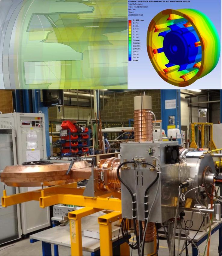
R r=1 a cyclotron (Kleeven et al., 2013). The RotCo is composed
R ⇣ ⇣ ⌘⌘ of a stator and a rotor with eight blades and rotates at a con-
1 X
reddtw (xi , xj ) = exp
(r) (r)
d x i , xj (22) stant speed of 7500 RPM with the help of ball bearings. A
R r=1 picture of the system is shown in Figure 3. Several sensors
are placed inside the machine to gather data. An accelerom-
7I NTERNATIONAL J OURNAL OF P ROGNOSTICS AND H EALTH M ANAGEMENT
input : Dataset: x = {x(1) , . . . , x(R) } where
x(r) 2 Rnr ⇥N , features (list of name of the
features), w1 = w2 = w3 = 13 ,
trendability method, redundancy method
(redcorr , redM I or reddtw via eq. (20-22)), nf
(number of features to keep), objective (OFD
via eq. (4) or OFQ via eq. (5))
rel = [] // relevance: empty array
red mat = 0 // redundancy matrix of size
N ⇥ N initialized with zeros
ranked features = [] // empty array
for i in 1,...,size(features) do
/* Relevance computation */
m = M (xi ) (via eq. 8) // monotonicity
p = P (xi ) (via eq. 9) // prognosability
t = T (xi ) (via eq. 11 or 13 depending on
trendability method) // trendability
m min(m)
rel[i] = w1 · max(m) min(m) + w2 ·
p min(p)
+ w3 · t min(t)
(eq. 14) Figure 3. (bottom) RF system of the cyclotron with the rotat-
max(p) min(p) max(t) min(t)
ing condenser on the right. (Top) Detailed view on the rotat-
/* Redundancy computation */ ing condenser. (Kleeven et al., 2013) CC-BY-3.0
for j in i+1,...,size(features) do
red mat[i, j] = redundancymethod (xi , xj )
end eter sensor is placed on the condenser to measure vibrations
end and performs 10-second acquisitions at a rate of 10kHz ev-
/* Heuristic search ery hour. Other sensors are placed on the machine to gather
*/
ranked features.append(arg maxi rel) // append data every second. Those include temperature sensors, vac-
the feature with maximum relevance to uum pressure and a torque sensor. In total, we have gathered
ranked features R = 11 run-to-failure time series.
features.pop(arg maxi rel) // Remove that
feature from the feature set After this data acquisition step, several health indicators (fea-
while size(features) < nf do tures) are constructed. For the vibration data, time-domain
score = [] (empty array) and frequency-domain features on each of the 10-second ac-
for f in features do quisition files are constructed. For the time-domain, those
⌦ = ranked features [ f include Root mean square (RMS), Median absolute devia-
D = rel[i] tion (MAD) which is a robust measure of variability based on
P|⌦| 1 P|⌦|
j=i+1 |⌦|(|⌦| 1) red mat[i, j]
2
R = i=1 the deviations from the median, peak to peak values, skew-
score[f] = D R if objective is OFD else ness (third statistical moment) and kurtosis (fourth statistical
D/R if objective is OFQ moment). Those also include metrics based on the peaks of
end the signals: crest factor, clearance factor, shape factor, mar-
best feature = arg maxf score gin factor and max amplitude (for a detailed explanation on
ranked features.append(best feature) those features, the reader can refer to MathWorks (2021)).
features.pop(best feature) For the frequency-domain features, we construct the ampli-
end tudes at the fundamental frequency and its first 3 harmonics,
return ranked features the spectral power of all 20 Hz non-overlapping bands from
Algorithm 1: prognostic mRMR algorithm 0-5kHz and finally the amplitudes at characteristic bearing
frequencies (Schoen et al., 1995), i.e.
⇣ ⌘
n Db
• Ball Pass Frequency Outer Race: 2f 1 D p
cos
⇣ ⌘
nf Db
• Ball Pass Frequency Inner Race: 2 1 + Dp cos
8I NTERNATIONAL J OURNAL OF P ROGNOSTICS AND H EALTH M ANAGEMENT
⇣ ⌘
Dp f Db
• Ball spin frequency: 2Db 1 (D p
cos )2
⇣ ⌘
f Db
• Fundamental train frequency: 2 1 Dp cos
where Dp is the pitch diameter, Db the ball diameter, the
contact angle and n the amount of balls. The first 3 harmon-
ics of those characteristic frequencies are also included. For
the non-vibration data, we perform aggregations of the sig-
nals over a 1-hour time-window to match with the vibration
acquisition sampling. Those aggregations include the mean,
max, min, standard deviation, skewness and kurtosis values.
This finally results in N = 317 features (297 from vibration Figure 4. Comparison of the four variants to compute the
data and 24 from non-vibration data) computed every hour. trendability metric and its consequence on the relevance.
4.1.2. Evaluation of the feature selection’s performance
4.2. Comparing methods to compute the prognostic mRMR
The next step is the feature selection. While we can evaluate
In this section, the different methods for computing the prog-
the best set of features with the algorithm developed (Algo-
nostic mRMR algorithm are compared, as summarized by Ta-
rithm 1) for a given method, we cannot conclude which one
ble 1. Subsection 4.2.1 compares the relevance criteria asso-
works better in practice nor how many features should be se-
ciated to the different choices in the trendability metric. Sub-
lected from the obtained ranked features.
section 4.2.2 compares the redundancy strategies and the final
subsection compares the two objective function formulations.
Hence, the prediction problem is formulated as a binary clas-
sification where the machine is either in a healthy state or a
4.2.1. Relevance measures
faulty state and we compare the approaches and the number of
features to be selected based on the classification score. How- The different strategies to compute the trendability metric and
ever, in practice we do not know when the machine enters a hence to compute the relevance of the features are compared.
faulty state. In this case, based on engineering expertise, we We assume that we want to keep at most 100 features for
assume that the machine is likely to be in a faulty state about computational, interpretability and stability reasons. For each
5 days before the failure. Moreover, we assume that the ma- number of selected features k between 10 and 100, we report
chine is in a healthy state from the beginning of its life until on Figure 4 the cross-validated F1 score associated to the se-
15 days prior to failure. 10 days of data for which we are the lection of k best features in terms of their relevance score (see
most unsure are thus excluded. This results in two artificial eq. 15). The process is repeated for the four strategies to com-
classes on which a classification can be performed. Note that pute the trendability as presented in section 3.
in section 4.3.2, other labelling strategies, i.e. different than
the 5-day time window, are tested. We observe no significant difference between the four ap-
proaches proposed except from 20 to 40 features selected,
The classification task is performed with a Support Vector where the DTW approach is outperforming the others. Al-
Machine (SVM) algorithm using a RBF kernel (see e.g. Hearst though a test for consistency on other data should be per-
et al. (1998)) which is a suitable classifier for this task. Fur- formed to confirm the trend, DTW seems to be a good can-
thermore, since there are only a few instances of failures in didate for comparing the features of different machines and
our dataset, a leave-one-out cross-validation is performed where hence for evaluating the relevance of a feature. In addition
each fold is defined as a run-to-failure time series. The clas- to the observed positive trend, DTW uses the time structure
sification score is averaged on the 11 folds of the dataset. No of the features and can map any instant in the time series of
hyperparameter tuning is performed on the SVM as the goal a particular machine to any other instant in another machine.
of this article is not to obtain the best prediction capabilities Indeed, intuitively, the start of a degradation phase in a spe-
but to compare different feature selection scenarios. The clas- cific machine will most likely never occur at the exact same
sification score chosen is the F1 score which is the harmonic time in another machine. This is where the correlation mea-
mean between the precision and recall, as it is a robust mea- sure (on which the other three methods are based) fails by
sure against imbalanced datasets (few failure data compared only being able to compare pairs of points at equivalent in-
to healthy data). dexes between two time series.
9I NTERNATIONAL J OURNAL OF P ROGNOSTICS AND H EALTH M ANAGEMENT
4.2.2. Redundancy measures
This section aims at improving the selection of features by
considering the redundancy between features and comparing
the proposed redundancy measures. In a first analysis we
choose to use the DTW approach for the trendability and rel-
evance computation as it resulted in the best score. We com-
pare the different relevance-redundancy scenarios as well as
the no redundancy scenario (based only on the relevance cri-
terion) and choose the OFD as the objective function. The
results are reported in Figure 5a. We observe that taking
into account redundancy does not improve and actually de-
creases the effectiveness of our model for 10 to 40 features.
For more features considered however, the relevance-only ap-
proach performs slightly worse than the others. This can be
explained by the fact that the other approaches tend to select (a) Using all features.
features that are sometimes not relevant only because they are
highly independent from each other. An improved approach
taking the best of both worlds is to preselect features that
are at least above a certain relevance threshold or to define
a threshold on the maximum number of features to preselect.
In the next analysis the 100 most relevant features are pres-
elected according to their fitness score. The same compari-
son as in Figure 5a is performed with those 100 preselected
features. The results are shown in Figure 5b. We can ob-
serve that the DTW approach now outperforms the relevance
only approach by a small margin and reaches an overall max-
imum score of 0.78 for 30 selected features. For the corre-
lation and mutual information approaches however, they still
are not able to achieve better performance than the relevance
only approach but they show better performance when 40 to (b) Using only the 100 most relevant features
70 features are selected and similar performance when more Figure 5. Comparison of relevance-only approach (None in
than 70 features are selected. The conclusion from Figure 5 green) and the 3 mRMR approaches with trendability metric
is that taking into account redundancy between features can computed via DTW.
definitely help, but a careful preselection should be done first
to exclude highly irrelevant features. Moreover, as a recom- 4.3. Comparison of our method with existing methods
mendation, we propose to compute the redundancy between
features via the DTW measure as it yields good and stable This section compares our prognostic mRMR algorithm with
results. existing feature selection methods proposed in the literature.
The prognostic mRMR is computed with the measures that
4.2.3. Objective function formulations give the best results on the case study, i.e. with the trend-
ability metric and redundancy measure computed via the dy-
Based on the best approach obtained so far (trendability and namic time warping measure, OFD chosen as the objective
redundancy computed with DTW approach), we compare the function and a preselection of the best 100 features accord-
two objective function formulations: OFD (eq. 4) and OFQ ing to their fitness score. In section 4.3.1, we compare our
(eq. 5). The results are reported in Figure 6. We observe no approach with the feature selection based on the prognostic
impact on the outcome for the choice of the objective func- metrics of Coble, J. B. (2010). In section 4.3.2, we compare
tion formulation except for a slightly better performance with our approach with the conventional mRMR feature selection.
OFD when 30 features are selected, which is likely negligi-
ble. Since the conventional way to formulate the mRMR is 4.3.1. Comparison with feature selection based on the prog-
via OFD, we propose to keep this formulation. nostic metrics from Coble
A comparison between our prognostic mRMR algorithm and
the feature selection based on the three original metrics de-
fined by Coble, J. B. (2010) is shown in Figure 7. We can
10I NTERNATIONAL J OURNAL OF P ROGNOSTICS AND H EALTH M ANAGEMENT
labelling is not available but we can use the class label based
on the window labelling described in section 4.1.2.
The labels defining a faulty state were defined somewhat arbi-
trarily based on engineering expertise. Hence, to fully com-
pare the classical mRMR with our prognostic mRMR algo-
rithm, we compare them for different labelling strategies: 10
different labelling strategies where the machine is consid-
ered in a faulty state starting n days before the failure where
n = 1, 2, ..., 10 are compared. The healthy state spans from
machine installation time to 15 days prior to failure as de-
tailed in section 4.1.2. For each labelling strategy, the cross-
validated F1 score is compared for a number of features rang-
ing from 10 to 100. The results are outlined in Figure 8. To
assess the two approaches, we either consider the global re-
sults by comparing the two curves, or refer to the maximal
Figure 6. Comparison of the two objective function formula-
tion: OFD (see eq. 4) and OFQ (see eq. 5) score attained for any number of features for each of the la-
belling strategies. For the latter, we simply need to compare
the maximum point on each curve while for the former op-
tion, we can either compare the sum of differences (SD) be-
tween scores corresponding to the same number of features,
or the number of times one curve is above the other (N D),
based on the 10 scores computed for the increasing feature
set size. Mathematically, this is:
X
SD = F1prognostic (i) F1classical (i)
i2{10,20,...,100}
n o
N D = # i 2 {10, 20, ..., 100}: F1prognostic (i) > F1classical (i)
where F1prognostic (i) and F1classical (i) are the cross-validated F1
score associated to the feature set of size i computed via the
prognostic mRMR algorithm and the classical mRMR algo-
rithm respectively. The prognostic mRMR should be supe-
Figure 7. Comparison of the prognostic mRMR with the fea- rior to the classical mRMR if SD > 0 or N D > 5 for a
ture selection from Coble & Hines (2009). particular labelling strategy. Table 2 summarizes the results
and individual scores are outlined in Figure 8. From a global
standpoint, the prognostic approach outperforms the classical
clearly observe that our method selects a subset of features approach in 9 out of 10 cases with respect to the SD metric
that is better able to discriminate between a faulty and healthy and 7 out of 9 cases + 1 ex aequo with respect to the N D met-
state (F1 score is higher), regardless of the chosen number ric. If we only look at the maximum values, the best result is
of features. This may be explained by two reasons. First, split among the two approaches (5 cases for both). Moreover,
redundancy is taken into account in the prognostic mRMR prognostic mRMR is consistently better with fewer features
approach while it is not in Coble’s approach. Second, the and thus is able to select the best compact set of features for
prognostic metrics used in the prognostic mRMR are more the prognostic task.
robust that the ones in Coble. Indeed, this can be observed
when comparing Coble’s approach (the solid black line from 5. C ONCLUSION
Figure 7) with the relevance only version of our prognostic
mRMR (green dotted line from Figure 5). We developed an unsupervised minimum redundancy maxi-
mum relevance feature selection method for predictive main-
4.3.2. Comparison with the classical mRMR approach tenance applications by adapting the conventional mRMR al-
gorithm where the relevance of a feature is computed with
The classical use of the mRMR algorithm requires to compute respect to prognostic metrics instead of class labels. We also
the relevance of the features based on the class labels, usually compared different measures to compute the redundancy be-
labelled machine malfunctions such as inner and outer ring tween features and adapted existing metrics quantifying the
defects in the case of bearings. In our application, such rich
11I NTERNATIONAL J OURNAL OF P ROGNOSTICS AND H EALTH M ANAGEMENT
Label [days] SD ND max score proach. In Annual conference of the prognostics and health
1 1.02 8 prognostic management society (Vol. 27).
2 0.69 5 prognostic
3 1.16 7 prognostic Coble, J. B. (2010). Merging data sources to predict remain-
4 0.71 7 classical ing useful life–an automated method to identify prognostic
5 0.04 4 classical parameters. (PhD thesis)
6 -0.08 3 classical
7 0.47 7 classical Ding, C., & Peng, H. (2005). Minimum redundancy feature
8 0.46 6 classical selection from microarray gene expression data. Journal
9 0.88 10 prognostic of bioinformatics and computational biology, 3(02), 185–
10 0.74 8 prognostic 205.
Table 2. Results of classical vs. prognostic mRMR. Results Fernandes, M., Canito, A., Bolón-Canedo, V., Conceição, L.,
are highlighted in bold when the prognostic approach outper- Praça, I., & Marreiros, G. (2019). Data analysis and feature
forms the classical mRMR approach. Prognostic mRMR is selection for predictive maintenance: A case-study in the
better if SD > 0 and N D > 5. metallurgic industry. International journal of information
management, 46, 252–262.
relevance of features. We performed a case study for a rotat- Gel’Fand, I., & Yaglom, A. (1959). Calculation of the amount
ing machine that highlighted the superiority of our feature of information abouta random function contained in an-
selection method compared to previous prognostic metrics other such function. Eleven Papers on Analysis, Proba-
and the conventional mRMR algorithm, especially for select- bility and Topology, 12, 199.
ing a compact set of features. We also showed that dynamic Giorgino, T., et al. (2009). Computing and visualizing dy-
time warping is a well-suited distance measure for predictive namic time warping alignments in r: the dtw package.
maintenance applications that can help to select a good set of Journal of statistical Software, 31(7), 1–24.
features. Hearst, M. A., Dumais, S. T., Osuna, E., Platt, J., &
Scholkopf, B. (1998). Support vector machines. IEEE
The approaches presented in this paper may still be improved Intelligent Systems and their applications, 13(4), 18–28.
by seeking the best parameters in the fitness metric charac- Hu, Q., Si, X.-S., Qin, A.-S., Lv, Y.-R., & Zhang, Q.-H.
terizing the relevance of a feature as well as the weights as- (2020). Machinery fault diagnosis scheme using redefined
signed to the relevance and redundancy in the objective func- dimensionless indicators and mrmr feature selection. IEEE
tion, which we leave to future work. Access, 8, 40313–40326.
Javed, K., Gouriveau, R., Zerhouni, N., & Nectoux, P. (2013).
ACKNOWLEDGEMENT
A feature extraction procedure based on trigonometric
This work was supported by the Biowin BiDMed project funded functions and cumulative descriptors to enhance prognos-
by the Walloon Region. The authors are very thankful to the tics modeling. In 2013 ieee conference on prognostics and
three reviewers whose insightful and constructive comments health management (phm) (pp. 1–7).
greatly helped improve the paper. Javed, K., Gouriveau, R., Zerhouni, N., & Nectoux, P. (2014).
Enabling health monitoring approach based on vibration
data for accurate prognostics. IEEE Transactions on In-
R EFERENCES dustrial Electronics, 62(1), 647–656.
Camci, F., Medjaher, K., Zerhouni, N., & Nectoux, P. (2013). Kleeven, W., Abs, M., Forton, E., Henrotin, S., Jongen, Y.,
Feature evaluation for effective bearing prognostics. Qual- Nuttens, V., . . . others (2013). The IBA superconducting
ity and reliability engineering international, 29(4), 477– synchrocyclotron project S2C2. In Proc. cyclotrons (pp.
486. 115–119).
Carino, J. A., Zurita, D., Delgado, M., Ortega, J., & Romero- Kraskov, A., Stögbauer, H., & Grassberger, P. (2004). Es-
Troncoso, R. (2015). Remaining useful life estimation of timating mutual information. Physical review E, 69(6),
ball bearings by means of monotonic score calibration. In 066138.
2015 ieee international conference on industrial technol- Lei, Y., Li, N., Gontarz, S., Lin, J., Radkowski, S., & Dybala,
ogy (icit) (pp. 1752–1758). J. (2016). A model-based method for remaining useful life
prediction of machinery. IEEE Transactions on Reliability,
Chandrashekar, G., & Sahin, F. (2014). A survey on feature 65(3), 1314–1326.
selection methods. Computers & Electrical Engineering,
Lei, Y., Li, N., Guo, L., Li, N., Yan, T., & Lin, J. (2018).
40(1), 16–28.
Machinery health prognostics: A systematic review from
Coble, J., & Hines, J. W. (2009). Identifying optimal data acquisition to rul prediction. Mechanical Systems and
prognostic parameters from data: a genetic algorithms ap- Signal Processing, 104, 799–834.
12I NTERNATIONAL J OURNAL OF P ROGNOSTICS AND H EALTH M ANAGEMENT
Li, N., Lei, Y., Liu, Z., & Lin, J. (2014). A particle filtering- Yan, X., & Jia, M. (2019). Intelligent fault diagnosis of ro-
based approach for remaining useful life predication of tating machinery using improved multiscale dispersion en-
rolling element bearings. In 2014 international conference tropy and mrmr feature selection. Knowledge-Based Sys-
on prognostics and health management (pp. 1–8). tems, 163, 450–471.
Li, Y., Yang, Y., Li, G., Xu, M., & Huang, W. (2017). A fault Zhang, B., Zhang, L., & Xu, J. (2016). Degradation feature
diagnosis scheme for planetary gearboxes using modified selection for remaining useful life prediction of rolling el-
multi-scale symbolic dynamic entropy and mrmr feature ement bearings. Quality and Reliability Engineering Inter-
selection. Mechanical Systems and Signal Processing, 91, national, 32(2), 547–554.
295–312. Zhang, X., Song, Z., Li, D., Zhang, W., Zhao, Z., & Chen, Y.
Liu, Z., Zuo, M. J., & Qin, Y. (2016). Remaining useful (2018). Fault diagnosis for reducer via improved lmd and
life prediction of rolling element bearings based on health svm-rfe-mrmr. Shock and Vibration, 2018.
state assessment. Proceedings of the Institution of Mechan- Zhao, X., Zuo, M. J., Liu, Z., & Hoseini, M. R. (2013). Diag-
ical Engineers, Part C: Journal of Mechanical Engineering nosis of artificially created surface damage levels of planet
Science, 230(2), 314–330. gear teeth using ordinal ranking. Measurement, 46(1),
Liu, Z., Zuo, M. J., & Xu, H. (2013). Fault diagnosis for plan- 132–144.
etary gearboxes using multi-criterion fusion feature selec-
tion framework. Proceedings of the Institution of Mechani-
cal Engineers, Part C: Journal of Mechanical Engineering B IOGRAPHIES
Science, 227(9), 2064–2076. Valentin Hamaide is a PhD student in the ICTEAM insti-
MathWorks. (2021). Signal features - matlab & simulink. Re- tute of the Université Catholique de Louvain. He received his
trieved 2021-03-22, from https://mathworks.com/ master’s degree in mathematical engineering in 2017 in the
help/predmaint/ug/signal-features.html same university. His research interests are machine learning
Peng, H., Long, F., & Ding, C. (2005). Feature se- and optimization with applications in the medical domain.
lection based on mutual information: Criteria of Max-
Dependency, Max-Relevance, and Min-Redundancy. IEEE François Glineur received dual engineering degrees from
Transactions on Pattern Analysis and Machine Intelli- Université de Mons and CentraleSuplec in 1997, and a PhD
gence, 27(8), 1226–1238. doi: 10.1109/TPAMI.2005.159 in Applied Sciences from Université de Mons in 2001. He
visited Delft University of Technology and McMaster Uni-
Radovic, M., Ghalwash, M., Filipovic, N., & Obradovic, Z.
versity as a post-doctoral researcher, then joined Université
(2017). Minimum redundancy maximum relevance fea-
catholique de Louvain where he is currently a professor of
ture selection approach for temporal gene expression data.
applied mathematics at the Engineering School, member of
BMC bioinformatics, 18(1), 1–14.
the Center for Operations Research and Econometrics and the
Ross, B. C. (2014). Mutual information between discrete and Institute of Information and Communication Technologies,
continuous data sets. PloS one, 9(2), e87357. Electronics and Applied Mathematics. His research interests
Schoen, R. R., Habetler, T. G., Kamran, F., & Bartfield, R. focus on optimization models and methods (mainly convex
(1995). Motor bearing damage detection using stator cur- optimization and algorithmic efficiency) and their engineer-
rent monitoring. IEEE transactions on industry applica- ing applications, as well as on nonnegative matrix factoriza-
tions, 31(6), 1274–1279. tion and applications to data analysis.
Shahidi, P., Maraini, D., & Hopkins, B. (2016). Railcar
diagnostics using minimal-redundancy maximumrelevance
feature selection and support vector machine classification.
International Journal of Prognostics and Health Manage-
ment, 7, 2153–2648.
Solorio-Fernández, S., Carrasco-Ochoa, J. A., & Martı́nez-
Trinidad, J. F. (2020). A review of unsupervised feature
selection methods. Artificial Intelligence Review, 53(2),
907–948.
Tang, X., He, Q., Gu, X., Li, C., Zhang, H., & Lu, J. (2020).
A novel bearing fault diagnosis method based on gl-mrmr-
svm. Processes, 8(7), 784.
Wang, D., Tsui, K.-L., & Miao, Q. (2017). Prognostics and
health management: A review of vibration based bearing
and gear health indicators. Ieee Access, 6, 665–676.
13I NTERNATIONAL J OURNAL OF P ROGNOSTICS AND H EALTH M ANAGEMENT
Figure 8. Classical vs. prognostic mRMR feature selection for various labelling strategies.
14You can also read